跳到论文正文
W Papers独立论文阅读器 arXiv:1003.2710 论文正文 计算阅读时间 · 0%
引用这篇论文根据当前论文元数据生成,正式投稿前建议核对。


License: arXiv.org perpetual non-exclusive license
arXiv:1003.2710v2 [math.CO] 04 Apr 2010

Modular kk-noncrossing diagrams

Christian M. Reidys⋆{}^{\,\star}, Rita R. Wang and Albus Y. Y. Zhao

Center for Combinatorics, LPMC-TJKLC

Nankai University

Tianjin 300071

P.R. China

Phone: *86-22-2350-6800

Fax: *86-22-2350-9272

duck@santafe.edu

Abstract

In this paper we compute the generating function of modular, kk-noncrossing diagrams. A kk-noncrossing diagram is called modular if it does not contains any isolated arcs and any arc has length at least four. Modular diagrams represent the deformation retracts of RNA pseudoknot structures [5, 8, 10] and their properties reflect basic features of these bio-molecules. The particular case of modular noncrossing diagrams has been extensively studied [20, 21, 13, 6]. Let 𝖰k​(n){\sf Q}_{k}(n) denote the number of modular kk-noncrossing diagrams over nn vertices. We derive exact enumeration results as well as the asymptotic formula 𝖰k​(n)∼ck​n−(k−1)2−k−12​γk−n{\sf Q}_{k}(n)\sim c_{k}n^{-(k-1)^{2}-\frac{k-1}{2}}\gamma_{k}^{-n} for k=3,…,9k=3,\ldots,9 and derive a new proof of the formula 𝖰2(n)∼1.4848n−3/2 1.8489−n{\sf Q}_{2}(n)\sim 1.4848\,n^{-3/2}\,1.8489^{-n} [6].

Keywords: kk-noncrossing diagram, generating function, shape, symbolic enumeration, singularity analysis.

1. Introduction

The main result of this paper is the computation of the generating function of modular kk-noncrossing diagrams, 𝐐k​(z){\bf Q}_{k}(z). A diagram is a labeled graph over the vertex set [n]={1,…,n}[n]=\{1,\dots,n\} with vertex degrees not greater than one. The standard representation of a diagram is derived by drawing its vertices in a horizontal line and its arcs (i,j)(i,j) in the upper half-plane. A kk-crossing is a set of kk distinct arcs (i1,j1),(i2,j2),…,(ik,jk)(i_{1},j_{1}),(i_{2},j_{2}),\ldots,(i_{k},j_{k}) with the property

i1<i2<…<ik<j1<j2<…<jk.i_{1}<i_{2}<\ldots<i_{k}<j_{1}<j_{2}<\ldots<j_{k}.

Similarly a kk-nesting is a set kk distinct such arcs such that

i1<i2<…<ik<jk<…​j2<j1.i_{1}<i_{2}<\ldots<i_{k}<j_{k}<\ldots j_{2}<j_{1}.

Let A,BA,B be two sets of arcs, then AA is nested in BB if any element of AA is nested in any element of BB. A diagram without any kk-crossings is called a kk-noncrossing diagram. The length of an arc, (i,j)(i,j), is s=j−is=j-i, and we refer to such arc as ss-arc. Furthermore,

  • •

    a stack of length σ\sigma, Si,jσS_{i,j}^{\sigma}, is a maximal sequence of “parallel” arcs. A diagram, in which any arc is contained in a ss-stack, where s≥2s\geq 2 is called a canonical diagram,

    ((i,j),(i+1,j−1),…,(i+(σ−1),j−(σ−1))).((i,j),(i+1,j-1),\dots,(i+(\sigma-1),j-(\sigma-1))).

    Si,jσS_{i,j}^{\sigma} is also referred to as a σ\sigma-stack.

  • •

    a stem of size ss is a sequence

    (Si1,j1σ1,Si2,j2σ2,…,Sis,jsσs)\left(S_{i_{1},j_{1}}^{\sigma_{1}},S_{i_{2},j_{2}}^{\sigma_{2}},\ldots,S_{i_{s},j_{s}}^{\sigma_{s}}\right)

    where Sim,jmσmS_{i_{m},j_{m}}^{\sigma_{m}} is nested in Sim−1,jm−1σm−1S_{i_{m-1},j_{m-1}}^{\sigma_{m-1}} such that any arc nested in Sim−1,jm−1σm−1S_{i_{m-1},j_{m-1}}^{\sigma_{m-1}} is either contained or nested in Sim,jmσmS_{i_{m},j_{m}}^{\sigma_{m}}, for 2≤m≤s2\leq m\leq s.

  • •

    a hairpin-loop (loop) consists of an arc (i,j)(i,j) and a sequence of consecutive isolated vertices {i+1,i+2,…,j−1}\{i+1,i+2,\ldots,j-1\}, see Fig. 1.

Refer to caption
Fig. 1. Features of a modular 33-noncrossing diagram represented as planar graph (top) and in standard representation (bottom). We display a stack of length two (green), a stem of size two (red) and a hairpin-loop (purple).

RNA secondary structures [20, 21, 7, 22] are in the language of diagrams exactly modular, 22-noncrossing diagrams. In [8, 9, 10, 12], various classes of kk-noncrossing diagrams have been enumerated. However the approach employed in these papers does not work for modular kk-noncrossing diagrams. In contrast to the situation for RNA secondary structures, the combination of minimum arc length and canonicity poses serious difficulties. The main idea is to build modular kk-noncrossing diagrams via inflating their colored, 𝖵k{\sf V}_{k}-shapes, see Fig. 2. These shapes will be discussed in detail in Section 4. The inflation gives rise to “stem-modules” over shape-arcs and is the key for the symbolic derivation of 𝐐k​(z){\bf Q}_{k}(z). One additional observation maybe worth to be pointed out: the computation of the generating function of colored shapes in Section 4, hinges on the intuition that the crossings of short arcs are relatively simple and give rise to manageable recursions. The coloring of these shapes then allows to identify the arc-configurations that require special attention during the inflation process. Our results are of importance in the context of RNA pseudoknot structures [15] and evolutionary optimization [Reidys-Stadler-Combinatoriallandscapes-SiamReviews]. Furthermore they allow for conceptual proofs of the results in [4, 9, 10, 12].

Refer to caption
Fig. 2. Modular kk-noncrossing diagrams: the inflation method. A modular 33-noncrossing diagram (top) is derived by inflating its 𝖵3{\sf V}_{3}-shape (bottom) in two steps. First we individually inflate each shape-arc into a more complex configuration and second insert isolated vertices (purple).

The paper is organized as follows. In Section 2 we recall some basic facts on singularity analysis, the generating function of kk-noncrossing matchings, 𝖵k{\sf V}_{k}-shapes and symbolic enumeration. Since the results on kk-noncrossing matchings are difficult to recover from the literature or simply new but immaterial for our purposes, we present their proofs in the Supplemental Materials (SM). In Section 3 we analyze modular, noncrossing diagrams and in Section 4 we compute the generating function of colored shapes. Finally we prove the main theorem in Section 5.

2. Some basic facts

2.1. Singularity analysis

Oftentimes, we are given a generating function without having an explicit formula of its coefficients. Singularity analysis is a framework that allows to analyze the asymptotics of these coefficients. The key to the asymptotics of the coefficients are the singularities, which raises the question on how to locate them. In the particular case of power series f⁡(z)=∑n≥0an​znf(z)=\sum_{n\geq 0}a_{n}\,z^{n} with nonnegative coefficients and a radius of convergence R>0R>0, a theorem of Pringsheim [2, 17], guarantess a positive real dominant singularity at z=Rz=R. As we are dealing here with combinatorial generating functions we always have this dominant singularity. We shall prove that for all our generating functions it is the unique dominant singularity. The class of theorems that deal with the deduction of information about coefficients from the generating function are called transfer-theorems [2].

Theorem 1.

[2] Let [zn]​f​(z)[z^{n}]f(z) denote the nn-th coefficient of the power series f⁡(z)f(z) at z=0z=0.
(a) Suppose f⁡(z)=(1−z)−αf(z)=(1-z)^{-\alpha}, α∈ℂ∖ℤ≤0\alpha\in\mathbb{C}\setminus\mathbb{Z}_{\leq 0}, then

(2.1) [zn]​f​(z)\displaystyle[z^{n}]\,f(z) ∼\displaystyle\sim nα−1Γ⁡(α)[1+α⁡(α−1)2​n+α⁡(α−1)​(α−2)​(3​α−1)24​n2+\displaystyle\frac{n^{\alpha-1}}{\Gamma(\alpha)}\left[1+\frac{\alpha(\alpha-1)}{2n}+\frac{\alpha(\alpha-1)(\alpha-2)(3\alpha-1)}{24n^{2}}+\right.
α2​(α−1)2​(α−2)​(α−3)48​n3+O(1n4)].\displaystyle\qquad\quad\left.\frac{\alpha^{2}(\alpha-1)^{2}(\alpha-2)(\alpha-3)}{48n^{3}}+O\left(\frac{1}{n^{4}}\right)\right].

(b) Suppose f⁡(z)=(1−z)r​log⁡(11−z)f(z)=(1-z)^{r}\log(\frac{1}{1-z}), r∈ℤ≥0r\in\mathbb{Z}_{\geq 0}, then we have

(2.2) [zn]​f​(z)∼(−1)r​r!n⁡(n−1)​…​(n−r).[z^{n}]f(z)\sim\,(-1)^{r}\frac{r!}{n(n-1)\dots(n-r)}.

We use the notation

(2.3) (f⁡(z)=Θ⁡(g⁡(z))​as z→ρ)⟺(f⁡(z)/g⁡(z)→c​as z→ρ),\left(f(z)=\Theta\left(g(z)\right)\ \text{\rm as $z\rightarrow\rho$}\right)\ \Longleftrightarrow\ \left(f(z)/g(z)\rightarrow c\ \text{\rm as $z\rightarrow\rho$}\right),

where cc is some constant. We say a function f⁡(z)f(z) is Δρ\Delta_{\rho} analytic at its dominant singularity z=ρz=\rho, if it analytic in some domain Δρ(ϕ,r)={z∣|z|<r,z≠r,|Arg(z−ρ)|>ϕ}\Delta_{\rho}(\phi,r)=\{z\mid|z|<r,z\neq r,\,|{\rm Arg}(z-\rho)|>\phi\}, for some ϕ,r\phi,r, where r>|ρ|r>|\rho| and 0<ϕ<π20<\phi<\frac{\pi}{2}. Since the Taylor coefficients have the property

(2.4) ∀γ∈ℂ∖0;[zn]​f​(z)=γn​[zn]​f​(zγ),\forall\,\gamma\in\mathbb{C}\setminus 0;\quad[z^{n}]f(z)=\gamma^{n}[z^{n}]f(\frac{z}{\gamma}),

We can, without loss of generality, reduce our analysis to the case where z=1z=1 is the unique dominant singularity. The next theorem transfers the asymptotic expansion of a function near its unique dominant singularity to the asymptotic of the function’s coefficients.

Theorem 2.

[2] Let f⁡(z)f(z) be a Δ1\Delta_{1} analytic function at its unique dominant singularity z=1z=1. Let

g⁡(z)=(1−z)α​logβ⁡(11−z),α,β∈ℝ.g(z)=(1-z)^{\alpha}\log^{\beta}\left(\frac{1}{1-z}\right),\quad\alpha,\beta\in\mathbb{R}.

That is we have in the intersection of a neighborhood of 11

(2.5) f⁡(z)=Θ⁡(g⁡(z))for ​z→1.f(z)=\Theta(g(z))\quad\text{\it for }z\rightarrow 1.

Then we have

(2.6) [zn]​f​(z)=Θ⁡([zn]​g​(z)).[z^{n}]f(z)=\Theta\left([z^{n}]g(z)\right).

2.2. kk-noncrossing matchings

A kk-noncrossing matching is a kk-noncrossing diagram without isolated points. Let fk​(2​n)f_{k}(2n) denote the number of kk-noncrossing matchings. The exponential generating function of kk-noncrossing matchings satisfies the following identity [1, 3, 8]

(2.7) ∑n≥0fk​(2​n)⋅z2​n(2​n)!\displaystyle\sum_{n\geq 0}f_{k}(2n)\cdot\frac{z^{2n}}{(2n)!} =\displaystyle= det[Ii−j​(2​z)−Ii+j​(2​z)]|i,j=1k−1\displaystyle\det[I_{i-j}(2z)-I_{i+j}(2z)]|_{i,j=1}^{k-1}

where Ir​(2​z)=∑j≥0z2​j+rj!​(j+r)!I_{r}(2z)=\sum_{j\geq 0}\frac{z^{2j+r}}{{j!(j+r)!}} is the hyperbolic Bessel function of the first kind of order rr. Eq. (2.7) combined with the fact that recursions for the coefficients of the exponential generating function translate into recursions for the coefficients of the ordinary generating function, allows us to prove:

Lemma 1.

The generating function of kk-noncrossing matchings over 2​n2n vertices, 𝐅k​(z)=∑n≥0fk​(2​n)​zn{\bf F}_{k}(z)=\sum_{n\geq 0}f_{k}(2n)\,z^{n} is DD-finite, [16], i.e. there exists some e∈ℕe\in\mathbb{N} such that

(2.8) q0,k​(z)​ded​ze​𝐅k​(z)+q1,k​(z)​de−1d​ze−1​𝐅k​(z)+⋯+qe,k​(z)​𝐅k​(z)=0,q_{0,k}(z)\frac{d^{e}}{dz^{e}}{\bf F}_{k}(z)+q_{1,k}(z)\frac{d^{e-1}}{dz^{e-1}}{\bf F}_{k}(z)+\cdots+q_{e,k}(z){\bf F}_{k}(z)=0,

where qj,k​(z)q_{j,k}(z) are polynomials.

We sketch the proof of Lemma 1 in the SM.

Lemma 1 is of importance for two reasons: first any singularity of 𝐅k​(z){\bf F}_{k}(z) is contained in the set of roots of q0,k​(z)q_{0,k}(z) [16], which we denote by RkR_{k}. Second, the specific form of the ODE in eq. (2.8) is the key to derive the singular expansion of 𝐅k​(z){\bf F}_{k}(z), see Proposition 1 below.

We proceed by computing for 2≤k≤92\leq k\leq 9, the polynomials q0,k​(z)q_{0,k}(z) and their roots, see Table 1 and

kk q0,k​(z)q_{0,k}(z) RkR_{k}
22 (4​z−1)​z(4z-1)z {14}\{\frac{1}{4}\}
33 (16​z−1)​z2(16z-1)z^{2} {116}\{\frac{1}{16}\}
44 (144​z2−40​z+1)​z3(144z^{2}-40z+1)z^{3} {14,136}\{\frac{1}{4},\frac{1}{36}\}
55 (1024​z2−80​z+1)​z4(1024z^{2}-80z+1)z^{4} {116,164}\{\frac{1}{16},\frac{1}{64}\}
66 (14400​z3−4144​z2+140​z−1)​z5(14400z^{3}-4144z^{2}+140z-1)z^{5} {14,136,1100}\{\frac{1}{4},\frac{1}{36},\frac{1}{100}\}
77 (147456​z3−12544​z2+224​z−1)​z6(147456z^{3}-12544z^{2}+224z-1)z^{6} {116,164,1144}\{\frac{1}{16},\frac{1}{64},\frac{1}{144}\}
88 (2822400​z4−826624​z3+31584​z2−336​z+1)​z7(2822400z^{4}-826624z^{3}+31584z^{2}-336z+1)z^{7} {14,136,1100,1196}\{\frac{1}{4},\frac{1}{36},\frac{1}{100},\frac{1}{196}\}
99 (37748736​z4−3358720​z3+69888​z2−480​z+1)​z8(37748736z^{4}-3358720z^{3}+69888z^{2}-480z+1)z^{8} {116,164,1144,1256}\{\frac{1}{16},\frac{1}{64},\frac{1}{144},\frac{1}{256}\}

Table 1. We present the polynomials q0,k​(z)q_{0,k}(z) and their nonzero roots obtained by the MAPLE package GFUN.

observe that [11]

(2.9) fk​(2​n)∼c~k​n−((k−1)2+(k−1)/2)​(2​(k−1))2​n,c~k>0,k≥2.f_{k}(2n)\,\sim\,\widetilde{c}_{k}\,n^{-((k-1)^{2}+(k-1)/2)}\,(2(k-1))^{2n},\qquad\widetilde{c}_{k}>0,\,k\geq 2.

Equation (2.9) guarantees that 𝐅k​(z){\bf F}_{k}(z) has the unique dominant singularity ρk2\rho_{k}^{2}, where ρk=1/(2​k−2)\rho_{k}=1/(2k-2). According to Lemma 1, 𝐅k​(z){\bf F}_{k}(z) is DD-finite, whence we have analytic continuation in any simply connected domain containing zero avoiding its singularities [19]. As a result 𝐅k​(z){\bf F}_{k}(z) is Δρk2\Delta_{\rho_{k}^{2}} analytic as required by Theorem 2. Lemma 1 and eq. (2.9) put us in position to present the singular expansion of 𝐅k​(z){\bf F}_{k}(z):

Proposition 1.

For 2≤k≤92\leq k\leq 9, the singular expansion of 𝐅k​(z){\bf F}_{k}(z) for z→ρk2z\rightarrow\rho_{k}^{2} is given by

𝐅k​(z)={Pk​(z−ρk2)+ck′​(z−ρk2)((k−1)2+(k−1)/2)−1​log⁡(z−ρk2)​(1+o⁡(1))Pk​(z−ρk2)+ck′​(z−ρk2)((k−1)2+(k−1)/2)−1​(1+o⁡(1)),\begin{split}{\bf F}_{k}(z)=\begin{cases}P_{k}(z-\rho_{k}^{2})+c_{k}^{\prime}(z-\rho_{k}^{2})^{((k-1)^{2}+(k-1)/2)-1}\log(z-\rho_{k}^{2})\left(1+o(1)\right)\\ P_{k}(z-\rho_{k}^{2})+c_{k}^{\prime}(z-\rho_{k}^{2})^{((k-1)^{2}+(k-1)/2)-1}\left(1+o(1)\right),\end{cases}\end{split}

depending on kk being odd or even. Furthermore, the terms Pk​(z)P_{k}(z) are polynomials of degree not larger than (k−1)2+(k−1)/2−1(k-1)^{2}+(k-1)/2-1, ck′c_{k}^{\prime} is some constant, and ρk=1/(2​k−2)\rho_{k}=1/(2k-2).

We give the proof of Proposition 1 is the SM.

In our derivations the following instance of the supercritical paradigm [2] is of central importance: we are given a DD-finite function, f⁡(z)f(z) and an algebraic function g⁡(u)g(u) satisfying g⁡(0)=0g(0)=0. Furthermore we suppose that f⁡(g⁡(u))f(g(u)) has a unique real valued dominant singularity γ\gamma and gg is regular in a disc with radius slightly larger than γ\gamma. Then the supercritical paradigm stipulates that the subexponential factors of f⁡(g⁡(u))f(g(u)) at u=0u=0, given that g⁡(u)g(u) satisfies certain conditions, coincide with those of f⁡(z)f(z).

Theorem 1, Theorem 2 and Proposition 1 allow under certain conditions to obtain the asymptotics of the coefficients of supercritical compositions of the “outer” function 𝐅k​(z){\bf{F}}_{k}(z) and “inner” function ψ⁡(z)\psi(z).

Proposition 2.

Let ψ⁡(z)\psi(z) be an algebraic, analytic function in a domain 𝒟={z||z|≤r}\mathcal{D}=\{z||z|\leq r\} such that ψ⁡(0)=0\psi(0)=0. Suppose γ\gamma is the unique dominant singularity of 𝐅k​(ψ​(z)){\bf F}_{k}(\psi(z)) and minimum positive real solution of ψ⁡(γ)=ρk2\psi(\gamma)=\rho_{k}^{2}, |γ|<r|\gamma|<r, where ψ′​(γ)≠0\psi^{\prime}(\gamma)\neq 0. Then 𝐅k​(ψ​(z)){\bf F}_{k}(\psi(z)) has a singular expansion and

(2.10) [zn]​𝐅k​(ψ⁡(z))∼A​n−((k−1)2+(k−1)/2)​(1γ)n,[z^{n}]{\bf F}_{k}(\psi(z))\sim A\,n^{-((k-1)^{2}+(k-1)/2)}\left(\frac{1}{\gamma}\right)^{n},

where AA is some constant.

2.3. Shapes

Definition 1.

A 𝖵k{\sf V}_{k}-shape is a kk-noncrossing matching having stacks of length exactly one.

In the following we refer to 𝖵k{\sf V}_{k}-shape simply as shapes. That is, given a modular, kk-noncrossing diagram, δ\delta, its shape is obtained by first replacing each stem by an arc and then removing all isolated vertices, see Fig. 3.

Refer to caption

Fig. 3. From diagrams to shapes: A modular, 33-noncrossingd diagram (top-left) is mapped in two steps into its 𝖵3{\sf V}_{3}-shape (top-right). A stem (blue) is replaced by an single shape-arc (blue).

Let ℐk​(s,m){\mathcal{I}}_{k}(s,m) (ik​(s,m)i_{k}(s,m)) denote the set (number) of the 𝖵k{\sf V}_{k}-shapes with ss arcs and mm 11-arcs having the bivariate generating function

(2.11) 𝐈k​(z,u)=∑s≥0∑m=0sik​(s,m)​zs​um.{\bf I}_{k}(z,u)=\sum_{s\geq 0}\sum_{m=0}^{s}i_{k}(s,m)z^{s}u^{m}.

The bivariate generating function of ik​(s,m)i_{k}(s,m) and the generating function of 𝐅k​(z){\bf F}_{k}(z) are related as follows:

Lemma 2.

[14] Let kk be natural number where k≥2k\geq 2, then the generating function 𝐈k​(z,u){\bf I}_{k}(z,u) satisfy

(2.12) 𝐈k​(z,u)\displaystyle{\bf I}_{k}(z,u) =\displaystyle= 1+z1+2​z−z​u​𝐅k​(z⁡(1+z)(1+2​z−z​u)2).\displaystyle\frac{1+z}{1+2z-zu}{\bf F}_{k}\left(\frac{z(1+z)}{(1+2z-zu)^{2}}\right).

2.4. Symbolic enumeration

In the following we will compute the generating functions via the symbolic enumeration method [2]. For this purpose we need the notion of a combinatorial class. A combinatorial class (𝒞,w𝒞)(\mathcal{C},w_{\mathcal{C}}) is a set together with a size-function, w𝒞:𝒞⟶ℤ+w_{\mathcal{C}}\colon\mathcal{C}\longrightarrow\mathbb{Z}^{+} such that 𝒞n=w𝒞−1​(n)\mathcal{C}_{n}=w_{\mathcal{C}}^{-1}(n) is finite for any n∈ℤ+n\in\mathbb{Z}^{+}. We write ww instead of w𝒞w_{\mathcal{C}} and set Cn=|𝒞n|C_{n}=|\mathcal{C}_{n}|. Two special combinatorial classes are ℰ\mathcal{E} and 𝒵\mathcal{Z} which contain only one element of size 00 and 11, respectively. The generating function of a combinatorial class 𝒞\mathcal{C} is given by

(2.13) 𝐂⁡(z)=∑c∈𝒞zw⁡(c)=∑n≥0Cn​zn,{\bf{C}}(z)=\sum_{c\in\mathcal{C}}z^{w(c)}=\sum_{n\geq 0}C_{n}\,z^{n},

where 𝒞n⊂𝒞\mathcal{C}_{n}\subset\mathcal{C}. In particular, the generating functions of the classes ℰ\mathcal{E} and 𝒵\mathcal{Z} are 𝐄⁡(z)=1{\bf{E}}(z)=1 and 𝐙⁡(z)=z{\bf{Z}}(z)=z. Suppose 𝒞,𝒟\mathcal{C},\mathcal{D} are combinatorial classes. Then 𝒞\mathcal{C} is isomorphic to 𝒟\mathcal{D}, 𝒞≅𝒟\mathcal{C}\cong\mathcal{D}, if and only if ∀n≥0\forall\,n\geq 0,|𝒞n|=|𝒟n||\mathcal{C}_{n}|=|\mathcal{D}_{n}|. In the following we shall identify isomorphic combinatorial classes and write 𝒞=𝒟\mathcal{C}=\mathcal{D} if 𝒞≅𝒟\mathcal{C}\cong\mathcal{D}. We set

  • •

    𝒞+𝒟:=𝒞∪𝒟\mathcal{C}+\mathcal{D}:=\mathcal{C}\cup\mathcal{D}, if 𝒞∩𝒟=∅\mathcal{C}\cap\mathcal{D}=\varnothing and for α∈𝒞+𝒟\alpha\in\mathcal{C}+\mathcal{D},

    (2.14) w𝒞+𝒟(α)={w𝒞​(α)if​α∈𝒞w𝒟​(α)if​α∈𝒟.w_{\mathcal{C}+\mathcal{D}}(\alpha)=\left\{\begin{aligned} &w_{\mathcal{C}}(\alpha)\quad\text{if}\ \alpha\in\mathcal{C}\\ &w_{\mathcal{D}}(\alpha)\quad\text{if}\ \alpha\in\mathcal{D}.\end{aligned}\right.
  • •

    𝒞×𝒟:={α=(c,d)∣c∈𝒞,d∈𝒟}\mathcal{C}\times\mathcal{D}:=\{\alpha=(c,d)\mid c\in\mathcal{C},d\in\mathcal{D}\} and for α∈𝒞×𝒟\alpha\in\mathcal{C}\times\mathcal{D},

    (2.15) w𝒞×𝒟​((c,d))=w𝒞​(c)+w𝒟​(d).w_{\mathcal{C}\times\mathcal{D}}((c,d))=w_{\mathcal{C}}(c)+w_{\mathcal{D}}(d).

and furthermore 𝒞m:=∏h=1m𝒞\mathcal{C}^{m}:=\prod_{h=1}^{m}\mathcal{C} and Seq​(𝒞):=ℰ+𝒞+𝒞2+⋯\textsc{Seq}(\mathcal{C}):={\mathcal{E}}+\mathcal{C}+\mathcal{C}^{2}+\cdots. Plainly, Seq​(𝒞)\textsc{Seq}(\mathcal{C}) is a combinatorial class if and only if there is no element in 𝒞\mathcal{C} of size 00. We immediately observe

Proposition 3.

Suppose 𝒜\mathcal{A}, 𝒞\mathcal{C} and 𝒟\mathcal{D} are combinatorial classes with generating functions 𝐀⁡(𝐳){\bf{A}(z)}, 𝐂⁡(z){\bf{C}}(z) and 𝐃⁡(z){\bf{D}}(z). Then
(a) 𝒜=𝒞+𝒟⟹𝐀⁡(z)=𝐂⁡(z)+𝐃⁡(z)\mathcal{A}=\mathcal{C}+\mathcal{D}\Longrightarrow{\bf{A}}(z)={\bf{C}}(z)+{\bf{D}}(z)
(b) 𝒜=𝒞×𝒟⟹𝐀⁡(z)=𝐂⁡(z)⋅𝐃⁡(z)\mathcal{A}=\mathcal{C}\times\mathcal{D}\Longrightarrow{\bf{A}}(z)={\bf{C}}(z)\cdot{\bf{D}}(z)
(c) 𝒜=Seq​(𝒞)⟹𝐀⁡(z)=11−𝐂⁡(z)\mathcal{A}=\textsc{Seq}(\mathcal{C})\Longrightarrow{\bf{A}}(z)=\frac{1}{1-{\bf{C}}(z)}.

3. Modular, noncrossing diagrams

Let us begin by studying first the case k=2k=2 [6], where the asymptotic formula

𝖰2(n)∼1.4848⋅n−3/2⋅1.8489n,{\sf Q}_{2}(n)\sim 1.4848\cdot n^{-3/2}\cdot 1.8489^{n},

has been derived. In the following we extend the result in [6] by computing the generating function explicitely. The above asymptotic formula follows then easily by means of singularity analysis.

Proposition 4.

The generating function of modular, noncrossing diagrams is given by

(3.1) 𝐐2​(z)=1−z2+z41−z−z2+z3+2​z4+z6⋅𝐅2​(z4−z6+z8(1−z−z2+z3+2​z4+z6)2){\bf Q}_{2}(z)=\frac{1-z^{2}+z^{4}}{1-z-z^{2}+z^{3}+2z^{4}+z^{6}}\cdot{\bf F}_{2}\left(\frac{z^{4}-z^{6}+z^{8}}{(1-z-z^{2}+z^{3}+2z^{4}+z^{6})^{2}}\right)

and the coefficients 𝖰2​(n){\sf Q}_{2}(n) satisfy

𝖰2(n)∼c2n−3/2γ2−n,{\sf Q}_{2}(n)\sim c_{2}n^{-3/2}\gamma_{2}^{-n},

where γ2\gamma_{2} is the minimal, positive real solution of ϑ⁡(z)=1/4\vartheta(z)=1/4, and

(3.2) ϑ⁡(z)=z4−z6+z8(1−z−z2+z3+2​z4+z6)2.\vartheta(z)=\frac{z^{4}-z^{6}+z^{8}}{(1-z-z^{2}+z^{3}+2z^{4}+z^{6})^{2}}.

Here we have γ2≈1.8489\gamma_{2}\approx 1.8489 and c2≈1.4848c_{2}\approx 1.4848.

Proof.

Let 𝒬2{\mathcal{Q}}_{2} denote the set of modular noncrossing diagrams, ℐ2{\mathcal{I}}_{2} the set of all 𝖵2{\sf V}_{2}-shapes and ℐ2​(m){\mathcal{I}}_{2}(m) those having exactly mm 11-arcs. Then we have the surjective map

φ:𝒬2→ℐ2.\varphi\colon{\mathcal{Q}}_{2}\rightarrow{\mathcal{I}}_{2}.

The map φ\varphi is obviously surjective, inducing the partition 𝒬2=∪˙γ​φ−1​(γ){\mathcal{Q}}_{2}=\dot{\cup}_{\gamma}\varphi^{-1}(\gamma), where φ−1​(γ)\varphi^{-1}(\gamma) is the preimage set of shape γ\gamma under the map φ\varphi. Accordingly, we arrive at

(3.3) 𝐐2​(z)=∑m≥0∑γ∈ℐ2​(m)𝐐γ​(z).{\bf Q}_{2}(z)=\sum_{m\geq 0}\sum_{\gamma\in\,{\mathcal{I}}_{2}(m)}\mathbf{Q}_{\gamma}(z).

We proceed by computing the generating function 𝐐γ​(z)\mathbf{Q}_{\gamma}(z). We shall construct 𝐐γ​(z)\mathbf{Q}_{\gamma}(z) from certain combinatorial classes as “building blocks”. The latter are: ℳ\mathcal{M} (stems), 𝒦\mathcal{K} (stacks), 𝒩\mathcal{N} (induced stacks), ℒ\mathcal{L} (isolated vertices), ℛ\mathcal{R} (arcs) and 𝒵\mathcal{Z} (vertices), where 𝐙⁡(z)=z\mathbf{Z}(z)=z and 𝐑⁡(z)=z2\mathbf{R}(z)=z^{2}. We inflate γ∈ℐ2​(m)\gamma\in{\mathcal{I}}_{2}(m) having ss arcs, where s≥max⁡{1,m}s\geq\max\{1,m\}, to a modular noncrossing diagram in two steps.
Step I: we inflate any shape-arc to a stack of length at least 22 and subsequently add additional stacks. The latter are called induced stacks and have to be separated by means of inserting isolated vertices, see Fig. 4.
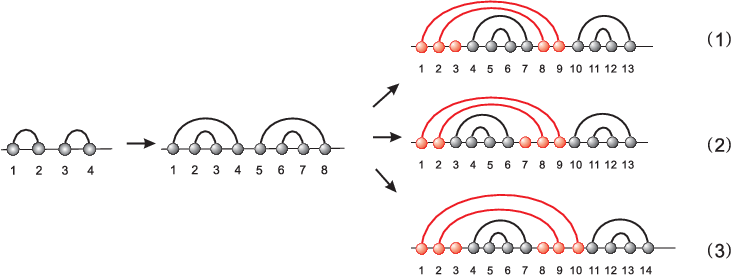
Refer to caption

Fig. 4. A shape (left) is inflated to a noncrossing, canonical diagram.

Note that during this first inflation step no intervals of isolated vertices, other than those necessary for separating the nested stacks are inserted. We generate

  • •

    sequences of isolated vertices ℒ=Seq​(𝒵)\mathcal{L}=\textsc{Seq}(\mathcal{Z}), where

    𝐋⁡(z)\displaystyle{\bf L}(z) =\displaystyle= 11−z\displaystyle\frac{1}{1-z}
  • •

    stacks, i.e.

    𝒦=ℛ2×Seq​(ℛ)\mathcal{K}=\mathcal{R}^{2}\times\textsc{Seq}\left(\mathcal{R}\right)

    with the generating function

    𝐊⁡(z)\displaystyle\mathbf{K}(z) =\displaystyle= z4⋅11−z2,\displaystyle z^{4}\cdot\frac{1}{1-z^{2}},
  • •

    induced stacks, i.e. stacks together with at least one nonempty interval of isolated vertices on either or both its sides.

    𝒩=𝒦×(𝒵×ℒ+𝒵×ℒ+(𝒵×ℒ)2)\mathcal{N}=\mathcal{K}\times\left(\mathcal{Z}\times\mathcal{L}+\mathcal{Z}\times\mathcal{L}+\left(\mathcal{Z}\times\mathcal{L}\right)^{2}\right)

    with generating function

    𝐍⁡(z)=z41−z2​(2​z1−z+(z1−z)2),\mathbf{N}(z)=\frac{z^{4}}{1-z^{2}}\left(2\frac{z}{1-z}+\left(\frac{z}{1-z}\right)^{2}\right),
  • •

    stems, that is pairs consisting of a stack 𝒦\mathcal{K} and an arbitrarily long sequence of induced stacks

    ℳ=𝒦×Seq​(𝒩)\mathcal{M}=\mathcal{K}\times\textsc{Seq}\left(\mathcal{N}\right)

    with generating function

    𝐌⁡(z)=𝐊⁡(z)1−𝐍⁡(z)=z41−z21−z41−z2​(2​z1−z+(z31−z)2).\displaystyle\mathbf{M}(z)=\frac{\mathbf{K}(z)}{1-\mathbf{N}(z)}=\frac{\frac{z^{4}}{1-z^{2}}}{1-\frac{z^{4}}{1-z^{2}}\left(2\frac{z}{1-z}+\left(\frac{z^{3}}{1-z}\right)^{2}\right)}.

Step II: we insert additional isolated vertices at the remaining (2​s+1)(2s+1) positions. For each 11-arc at least three such isolated vertices are necessarily inserted, see Fig. 5.

Refer to caption

Fig. 5. Step II: the noncrossing canonical diagram (left) obtained in (1) in Fig. 4 is inflated to a modular noncrossing diagram (right) by adding isolated vertices (red).

Combining Step I and Step II we arrive at

(3.4) 𝒬γ=(ℳ)s×ℒ2​s+1−m×(𝒵3×ℒ)m,\mathcal{Q}_{\gamma}=\left(\mathcal{M}\right)^{s}\times\mathcal{L}^{2s+1-m}\times\left(\mathcal{Z}^{3}\times\mathcal{L}\right)^{m},

where 𝒬γ\mathcal{Q}_{\gamma} is the combinatorial class of modular noncrossing diagrams having shape γ\gamma. Therefore,

𝐐γ​(z)\displaystyle{\bf Q}_{\gamma}(z) =\displaystyle= (z41−z21−z41−z2​(2​z1−z+(z1−z)2))s​(11−z)2​s+1−m​(z31−z)m\displaystyle\left(\frac{\frac{z^{4}}{1-z^{2}}}{1-\frac{z^{4}}{1-z^{2}}\left(2\frac{z}{1-z}+\left(\frac{z}{1-z}\right)^{2}\right)}\right)^{s}\left(\frac{1}{1-z}\right)^{2s+1-m}\left(\frac{z^{3}}{1-z}\right)^{m}
=\displaystyle= (1−z)−1​(z4(1−z2)​(1−z)2−(2​z−z2)​z4)s​(z3)m.\displaystyle(1-z)^{-1}\left(\frac{z^{4}}{(1-z^{2})(1-z)^{2}-(2z-z^{2})z^{4}}\right)^{s}\,(z^{3})^{m}.

Since for any γ,γ1∈ℐ2​(s,m)\gamma,\gamma_{1}\in\mathcal{I}_{2}(s,m) we have 𝐐γ​(z)=𝐐γ1​(z)\mathbf{Q}_{\gamma}(z)=\mathbf{Q}_{\gamma_{1}}(z), we derive

𝐐2​(z)=∑m≥0∑γ∈ℐ2​(m)𝐐γ​(z)=∑s≥0∑m=0si2​(s,m)​𝐐γ​(z).{\bf Q}_{2}(z)=\sum_{m\geq 0}\sum_{\gamma\in\,{\mathcal{I}}_{2}(m)}\mathbf{Q}_{\gamma}(z)=\sum_{s\geq 0}\sum_{m=0}^{s}i_{2}(s,m)\mathbf{Q}_{\gamma}(z).

We set

η⁡(z)=z4(1−z2)​(1−z)2−(2​z−z2)​z4\eta(z)=\frac{z^{4}}{(1-z^{2})(1-z)^{2}-(2z-z^{2})z^{4}}

and note that Lemma 2 guarantees

∑s≥0∑m=0si2​(s,m)​xs​ym\displaystyle\sum_{s\geq 0}\,\sum_{m=0}^{s}\,i_{2}(s,m)\,x^{s}\,y^{m} =\displaystyle= 1+x1+2​x−x​y​∑s≥0f2​(2​s,0)​(x⁡(1+x)(1+2​x−x​y)2)s.\displaystyle\frac{1+x}{1+2x-xy}\sum_{s\geq 0}f_{2}(2s,0)\left(\frac{x(1+x)}{(1+2x-xy)^{2}}\right)^{s}.

Therefore, setting x=η⁡(z)x=\eta(z) and y=z3y=z^{3} we arrive at

𝐐2​(z)=1−z2+z41−z−z2+z3+2​z4+z6⋅𝐅2​(z4−z6+z8(1−z−z2+z3+2​z4+z6)2)\displaystyle{\bf Q}_{2}(z)=\frac{1-z^{2}+z^{4}}{1-z-z^{2}+z^{3}+2z^{4}+z^{6}}\cdot{\bf F}_{2}\left(\frac{z^{4}-z^{6}+z^{8}}{(1-z-z^{2}+z^{3}+2z^{4}+z^{6})^{2}}\right)

By Lemma 1, 𝐐2​(z){\bf Q}_{2}(z) is DD-finite. Pringsheim’s Theorem [17] guarantees that 𝐐2​(z){\bf Q}_{2}(z) has a dominant real positive singularity γ2\gamma_{2}. We verify that γ2\gamma_{2} which is the unique solution of minimum modulus of the equation ϑ⁡(z)=ρ22\vartheta(z)=\rho_{2}^{2}, where ρ22\rho_{2}^{2} is the unique dominant singularity of 𝐅2​(z){\bf F}_{2}(z) and ρ2=1/2\rho_{2}=1/2. Furthermore we observe that γ2\gamma_{2} is the unique dominant singularity of 𝐐2​(z){\bf Q}_{2}(z), see the SM. It is straightforward to verify that ϑ′​(γ2)≠0\vartheta^{\prime}(\gamma_{2})\neq 0. According to Proposition 2, we therefore have

𝖰2(n)∼c2n−3/2γ2−n,{\sf Q}_{2}(n)\sim c_{2}n^{-3/2}\gamma_{2}^{-n},

and the proof of Proposition 4 is complete. ∎

4. Colored shapes

In the following we shall assume that k>2k>2, unless stated otherwise. The key to compute the generating function of modular kk-noncrossing diagrams are certain refinements of their 𝖵k{\sf V}_{k}-shapes. These refined shapes are called colored shapes and obtained by distinguishing a variety of crossings of 22-arcs, i.e. arcs of the form (i,i+2)(i,i+2). Each such class requires its specific inflation-procedure in Theorem 3.

Let us next have a closer look at these combinatorial classes (colors):

  • •

    𝐂1\mathbf{C}_{1} the class of of 11-arcs,

  • •

    𝐂2\mathbf{C}_{2} the class of arc-pairs consisting of mutually crossing 22-arcs,

  • •

    𝐂3\mathbf{C}_{3} the class of arc-pairs (α,β)(\alpha,\beta) where α\alpha is the unique 22-arc crossing β\beta and β\beta has length at least three.

  • •

    𝐂4\mathbf{C}_{4} the class of arc-triples (α1,β,α2)(\alpha_{1},\beta,\alpha_{2}), where α1\alpha_{1} and α2\alpha_{2} are 22-arcs that cross β\beta.

In Fig. 6 we illustrate how these classes are induced by modular kk-noncrossing diagrams.

Refer to caption
Fig. 6. Colored 𝖵k{\sf V}_{k}-shapes: a modular 33-noncrossing diagram (top) and its colored 𝖵3{\sf V}_{3}-shape (bottom). In the resulting 𝖵3{\sf V}_{3}-shape we color the four classes as follows: 𝐂1\mathbf{C}_{1}(green), 𝐂2\mathbf{C}_{2}(black), 𝐂3\mathbf{C}_{3}(blue) and 𝐂4\mathbf{C}_{4}(red).

Let us refine 𝖵k{\sf V}_{k}-shapes in two stages. For this purpose let ℐk​(s,u1,u2){\mathcal{I}}_{k}(s,u_{1},u_{2}) and ik​(s,u1,u2)i_{k}(s,u_{1},u_{2}) denote the set and cardinality of 𝖵k{\sf V}_{k}-shapes having ss arcs, u1u_{1} 11-arcs and u2u_{2} pairs of mutually crossing 22-arcs. Our first objective consists in computing the generating function

𝐖k​(x,y,w)=∑s≥0∑u1=0s∑u2=0⌊s−u12⌋ik​(s,u1,u2)​xs​yu1​wu2.{\bf W}_{k}(x,y,w)=\sum_{s\geq 0}\sum_{u_{1}=0}^{s}\sum_{u_{2}=0}^{\lfloor\frac{s-u_{1}}{2}\rfloor}i_{k}(s,u_{1},u_{2})\,x^{s}y^{u_{1}}w^{u_{2}}.

That is, we first take the classes 𝐂1\mathbf{C}_{1} and 𝐂2\mathbf{C}_{2} into account.

Lemma 3.

For k>2k>2, the coefficients ik​(s,u1,u2)i_{k}(s,u_{1},u_{2}) satisfy

(4.1) ik​(s,u1,u2)\displaystyle i_{k}(s,u_{1},u_{2}) =\displaystyle= 0for ​u1+2​u2>s\displaystyle 0\quad\text{for }u_{1}+2u_{2}>s
(4.2) ∑u2=0⌊s−u12⌋ik​(s,u1,u2)\displaystyle\sum_{u_{2}=0}^{\lfloor\frac{s-u_{1}}{2}\rfloor}i_{k}(s,u_{1},u_{2}) =\displaystyle= ik​(s,u1),\displaystyle i_{k}(s,u_{1}),

where ik​(s,u1)i_{k}(s,u_{1}) denotes the number of 𝖵k{\sf V}_{k}-shapes having ss arcs, u1u_{1} 11-arcs. Furthermore we have the recursion:

(4.3) (u2+1)​ik​(s+1,u1,u2+1)\displaystyle(u_{2}+1)i_{k}(s+1,u_{1},u_{2}+1) =\displaystyle= (u1+1)​ik​(s,u1+1,u2)\displaystyle(u_{1}+1)i_{k}(s,u_{1}+1,u_{2})
+(u1+1)​ik​(s−1,u1+1,u2).\displaystyle+(u_{1}+1)i_{k}(s-1,u_{1}+1,u_{2}).

The proof of Lemma 3 is given in SM. We next proceed by computing 𝐖k​(x,y,w){\bf W}_{k}(x,y,w).

Proposition 5.

For k>2k>2, we have

(4.4) 𝐖k​(x,y,w)=(1+x)​v​𝐅k​(x⁡(1+x)​v2),{\bf W}_{k}(x,y,w)=(1+x)v\,{\bf F}_{k}\left(x(1+x)v^{2}\right),

where v=((1−w)​x3+(1−w)​x2+(2−y)​x+1)−1v=\left((1-w)x^{3}+(1-w)x^{2}+(2-y)x+1\right)^{-1}.

Proof.

According to Lemma 2, we have

𝐈k​(z,u)=1+z1+2​z−z​u​𝐅k​(z⁡(1+z)(1+2​z−z​u)2).{\bf I}_{k}(z,u)=\frac{1+z}{1+2z-zu}{\bf F}_{k}\left(\frac{z(1+z)}{(1+2z-zu)^{2}}\right).

This generating function is connected to 𝐖k​(x,y,z){\bf W}_{k}(x,y,z) via eq. (4.2) of Lemma 3 as follows: setting w=1w=1, we have 𝐖k​(x,y,1)=𝐈k​(x,y){\bf W}_{k}(x,y,1)={\bf I}_{k}(x,y). The recursion of eq. (4.3) gives rise to the partial differential equation

(4.5) ∂𝐖k​(x,y,w)∂w\displaystyle\frac{\partial{\bf W}_{k}(x,y,w)}{\partial w} =\displaystyle= x​∂𝐖k​(x,y,w)∂y+x2​∂𝐖k​(x,y,w)∂y.\displaystyle x\frac{\partial{\bf W}_{k}(x,y,w)}{\partial y}+x^{2}\frac{\partial{\bf W}_{k}(x,y,w)}{\partial y}.

We next show

  • •

    the function

    (4.6) 𝐖k∗​(x,y,w)\displaystyle{\bf W}_{k}^{*}(x,y,w) =\displaystyle= (1+x)(1−w)​x3+(1−w)​x2+(2−y)​x+1×\displaystyle\frac{(1+x)}{(1-w)x^{3}+(1-w)x^{2}+(2-y)x+1}\times
    𝐅k​((1+x)​x((1−w)​x3+(1−w)​x2+(2−y)​x+1)2)\displaystyle{\bf F}_{k}\left(\frac{(1+x)x}{((1-w)x^{3}+(1-w)x^{2}+(2-y)x+1)^{2}}\right)\qquad

    is a solution of eq. (4.5),

  • •

    its coefficients, ik∗​(s,u1,u2)=[xs​yu1​wu2]​𝐖k∗​(x,y,w)i_{k}^{*}(s,u_{1},u_{2})=[x^{s}y^{u_{1}}w^{u_{2}}]{\bf W}_{k}^{*}(x,y,w), satisfy

    ik∗​(s,u1,u2)=0foru1+2​u2>s,i_{k}^{*}(s,u_{1},u_{2})=0\quad\text{for}\quad u_{1}+2u_{2}>s,
  • •

    𝐖k∗​(x,y,1)=𝐈k​(x,y){\bf W}_{k}^{*}(x,y,1)={\bf I}_{k}(x,y).

Firstly,

(4.7) ∂𝐖k∗​(x,y,w)∂y\displaystyle\frac{\partial{\bf W}^{*}_{k}(x,y,w)}{\partial y} =\displaystyle= u​𝐅k​(u)+2​u​𝐅k′​(u)\displaystyle u\,{\bf F}_{k}\left(u\right)+2u\,{\bf F}_{k}^{\prime}\left(u\right)
(4.8) ∂𝐖k∗​(x,y,w)∂w\displaystyle\frac{\partial{\bf W}^{*}_{k}(x,y,w)}{\partial w} =\displaystyle= x⁡(1+x)​u​𝐅k​(u)+2​x​(1+x)​u​𝐅k′​(u),\displaystyle x(1+x)u\,{\bf F}_{k}\left(u\right)+2x(1+x)u{\bf F}_{k}^{\prime}\left(u\right),

where

u=x⁡(1+x)((1−w)​x3+(1−w)​x2+(2−y)​x+1)2u=\frac{x(1+x)}{\left((1-w)x^{3}+(1-w)x^{2}+(2-y)x+1\right)^{2}}

and 𝐅k′​(u)=∑n≥0n​fk​(2​n)​(u)n{\bf F}_{k}^{\prime}\left(u\right)=\sum_{n\geq 0}nf_{k}(2n)(u)^{n}. Consequently, we derive

(4.9) ∂𝐖k∗​(x,y,w)∂w=x​∂𝐖k∗​(x,y,w)∂y+x2​∂𝐖k∗​(x,y,w)∂y.\frac{\partial{\bf W}_{k}^{*}(x,y,w)}{\partial w}=x\frac{\partial{\bf W}_{k}^{*}(x,y,w)}{\partial y}+x^{2}\frac{\partial{\bf W}_{k}^{*}(x,y,w)}{\partial y}.

Secondly we prove ik∗​(s,u1,u2)=0i_{k}^{*}(s,u_{1},u_{2})=0 for u1+2​u2>su_{1}+2u_{2}>s. To this end we observe that 𝐖k∗​(x,y,w){\bf W}^{*}_{k}(x,y,w) is a power series, since it is analytic in (0,0,0)(0,0,0). It now suffices to note that the indeterminants yy and ww only appear in form of products x​yxy and x2​wx^{2}w or x3​wx^{3}w. Thirdly, the equality 𝐖k∗​(x,y,1)=𝐈k​(x,y){\bf W}_{k}^{*}(x,y,1)={\bf I}_{k}(x,y) is obvious.
Claim.

(4.10) 𝐖k∗​(x,y,w)=𝐖k​(x,y,w).{\bf W}^{*}_{k}(x,y,w)={\bf W}_{k}(x,y,w).

By construction the coefficients ik∗​(s,u1,u2)i^{*}_{k}(s,u_{1},u_{2}) satisfy eq. (4.3) and we just proved ik∗​(s,u1,u2)=0i_{k}^{*}(s,u_{1},u_{2})=0 for u1+2​u2>su_{1}+2u_{2}>s. In view of 𝐖k∗​(x,y,1)=𝐈k​(x,y){\bf W}_{k}^{*}(x,y,1)={\bf I}_{k}(x,y) we have

∀s,u1;∑u2=0⌊s−u12⌋ik∗​(s,u1,u2)=ik​(s,u1).\forall\,s,u_{1};\qquad\sum_{u_{2}=0}^{\lfloor\frac{s-u_{1}}{2}\rfloor}i_{k}^{*}(s,u_{1},u_{2})=i_{k}(s,u_{1}).

Using these three properties it follows via induction over ss

∀s,u1,u2≥0;ik∗​(s,u1,u2)=ik​(s,u1,u2),\forall\,s,u_{1},u_{2}\geq 0;\qquad i_{k}^{*}(s,u_{1},u_{2})=i_{k}(s,u_{1},u_{2}),

whence the Claim and the proposition follows. ∎

In addition to 𝐂1\mathbf{C}_{1} and 𝐂2\mathbf{C}_{2}, we consider next the classes 𝐂3\mathbf{C}_{3} and 𝐂4\mathbf{C}_{4}. For this purpose we have to identify two new recursions, see Lemma 4. Setting u→=(u1,…,u4)\vec{u}=(u_{1},\dots,u_{4}) we denote by ℐk​(s,u→)\mathcal{I}_{k}(s,\vec{u}) and ik​(s,u→)i_{k}(s,\vec{u}), the set and number of colored 𝖵k{\sf V}_{k}-shapes over ss arcs, containing uiu_{i} elements of class 𝐂i\mathbf{C}_{i}, where 1≤i≤41\leq i\leq 4. The key result is

Lemma 4.

For k>2k>2, the coefficients ik​(s,u→)i_{k}(s,\vec{u}) satisfy

(4.11) ik​(s,u1,u2,u3,u4)\displaystyle i_{k}(s,u_{1},u_{2},u_{3},u_{4}) =\displaystyle= 0for ​u1+2​u2+2​u3+3​u4>s\displaystyle 0\quad\text{for }u_{1}+2u_{2}+2u_{3}+3u_{4}>s
(4.12) ∑u3,u4≥0ik​(s,u1,u2,u3,u4)\displaystyle\sum_{u_{3},u_{4}\geq 0}i_{k}(s,u_{1},u_{2},u_{3},u_{4}) =\displaystyle= ik​(s,u1,u2).\displaystyle i_{k}(s,u_{1},u_{2}).

Furthermore we have the recursions

(u3+1)\displaystyle(u_{3}+1) ik​(s+1,u1,u2,u3+1,u4)=\displaystyle i_{k}(s+1,u_{1},u_{2},u_{3}+1,u_{4})=
 2​u1​ik​(s−1,u1,u2,u3,u4)\displaystyle\quad\,2u_{1}i_{k}(s-1,u_{1},u_{2},u_{3},u_{4})
+4​(u2+1)​ik​(s−1,u1,u2+1,u3,u4)\displaystyle+4(u_{2}+1)i_{k}(s-1,u_{1},u_{2}+1,u_{3},u_{4})
+4​(u2+1)​ik​(s−1,u1,u2+1,u3−1,u4)\displaystyle+4(u_{2}+1)i_{k}(s-1,u_{1},u_{2}+1,u_{3}-1,u_{4})
+4​(u2+1)​ik​(s−2,u1,u2+1,u3−1,u4)\displaystyle+4(u_{2}+1)i_{k}(s-2,u_{1},u_{2}+1,u_{3}-1,u_{4})
+2​(u3+1)​ik​(s,u1,u2,u3+1,u4)\displaystyle+2(u_{3}+1)i_{k}(s,u_{1},u_{2},u_{3}+1,u_{4})
+2​u3​ik​(s−1,u1,u2,u3,u4)\displaystyle+2u_{3}i_{k}(s-1,u_{1},u_{2},u_{3},u_{4})
+6​(u3+1)​ik​(s−1,u1,u2,u3+1,u4)\displaystyle+{6(u_{3}+1)i_{k}(s-1,u_{1},u_{2},u_{3}+1,u_{4})}
+2​(u3+1)​ik​(s−2,u1,u2,u3+1,u4)\displaystyle+2(u_{3}+1)i_{k}(s-2,u_{1},u_{2},u_{3}+1,u_{4})
+2​u3​ik​(s−2,u1,u2,u3,u4)\displaystyle+2u_{3}i_{k}(s-2,u_{1},u_{2},u_{3},u_{4})
+4​(u4+1)​ik​(s,u1,u2,u3−1,u4+1)\displaystyle+4(u_{4}+1)i_{k}(s,u_{1},u_{2},u_{3}-1,u_{4}+1)
+4​(u4+1)​ik​(s−1,u1,u2,u3−1,u4+1)\displaystyle+4(u_{4}+1)i_{k}(s-1,u_{1},u_{2},u_{3}-1,u_{4}+1)
+4​u4​ik​(s−1,u1,u2,u3,u4)\displaystyle+4u_{4}i_{k}(s-1,u_{1},u_{2},u_{3},u_{4})
+4​(u4+1)​ik​(s−1,u1,u2,u3,u4+1)\displaystyle+4(u_{4}+1)i_{k}(s-1,u_{1},u_{2},u_{3},u_{4}+1)
+4​u4​ik​(s−2,u1,u2,u3,u4)\displaystyle+4u_{4}i_{k}(s-2,u_{1},u_{2},u_{3},u_{4})
+2​(u4+1)​ik​(s−2,u1,u2,u3,u4+1)\displaystyle+2(u_{4}+1)i_{k}(s-2,u_{1},u_{2},u_{3},u_{4}+1)
+(2​s−2​u1−4​u2−4​u3−6​u4)​ik​(s,u1,u2,u3,u4)\displaystyle+({2s}-2u_{1}-4u_{2}-4u_{3}-6u_{4})i_{k}(s,u_{1},u_{2},u_{3},u_{4})
+2​(2​(s−1)−2​u1−4​u2−4​u3−6​u4)​ik​(s−1,u1,u2,u3,u4)\displaystyle+2(2(s-1)-2u_{1}-4u_{2}-4u_{3}-6u_{4})i_{k}(s-1,u_{1},u_{2},u_{3},u_{4})
(4.13) +(2​(s−2)−4​u2−4​u3−6​u4)​ik​(s−2,u1,u2,u3,u4)\displaystyle+({2(s-2)}-4u_{2}-4u_{3}-6u_{4})i_{k}(s-2,u_{1},u_{2},u_{3},u_{4})

and

2​(u4+1)​ik​(s+1,u1,u2,u3,u4+1)\displaystyle 2(u_{4}+1)i_{k}(s+1,u_{1},u_{2},u_{3},u_{4}+1) =(u3+1)​ik​(s,u1,u2,u3+1,u4)\displaystyle=(u_{3}+1)i_{k}(s,u_{1},u_{2},u_{3}+1,u_{4})
(4.14) +2​(u2+1)k​(s,u1,u2+1,u3,u4).\displaystyle\quad+2(u_{2}+1)_{k}(s,u_{1},u_{2}+1,u_{3},u_{4}).\quad

The proof of Lemma 4 is presented the SM and follows by removing a specific arc in a labelled 𝐂3{\bf C}_{3}-element and careful accounting of the resulting arc-configurations.

Proposition 5 and Lemma 4 put us in position to compute the generating function of colored 𝖵k{\sf V}_{k}-shapes

(4.15) 𝐈k​(x,y,z,w,t)=∑s,u1,u2,u3,u4ik​(s,u→)​xs​yu1​zu2​wu3​tu4.{\bf I}_{k}(x,y,z,w,t)=\sum_{s,u_{1},u_{2},u_{3},u_{4}}i_{k}(s,\vec{u})\,x^{s}y^{u_{1}}z^{u_{2}}w^{u_{3}}t^{u_{4}}.
Proposition 6.

For k>2k>2, the generating function of colored 𝖵k{\sf V}_{k}-shapes is given by

(4.16) 𝐈k​(x,y,z,w,t)=1+xθ​𝐅k​(x⁡(1+(2​w−1)​x+(t−1)​x2)θ2),{\bf I}_{k}(x,y,z,w,t)=\frac{1+x}{\theta}{\bf F}_{k}\left(\frac{x(1+(2w-1)x+(t-1)x^{2})}{\theta^{2}}\right),

where θ=1−(y−2)​x+(2​w−z−1)​x2+(2​w−z−1)​x3\theta=1-(y-2)x+(2w-z-1)x^{2}+(2w-z-1)x^{3}.

Proof.

The first recursion of Lemma 4 implies the partial differential equation

∂𝐈k∂w\displaystyle\frac{\partial{\bf I}_{k}}{\partial w} =∂𝐈k∂x​(2​x2+4​x3+2​x4)−∂𝐈k∂y​(2​x​y+2​x2​y)\displaystyle=\frac{\partial{\bf I}_{k}}{\partial x}(2x^{2}+4x^{3}+2x^{4})-\frac{\partial{\bf I}_{k}}{\partial y}(2xy+2x^{2}y)
+∂𝐈k∂z​(−4​x​z+4​x2​w+4​x2−4​x3​z−8​x2​z+4​x3​w)\displaystyle+\frac{\partial{\bf I}_{k}}{\partial z}(-4xz+4x^{2}w+4x^{2}-4x^{3}z-8x^{2}z+4x^{3}w)
+∂𝐈k∂w​(−4​x​w+2​x−6​x2​w+6​x2−2​x3​w+2​x3)\displaystyle+\frac{\partial{\bf I}_{k}}{\partial w}(-4xw+2x-6x^{2}w+6x^{2}-2x^{3}w+2x^{3})
(4.17) +∂𝐈k∂t​(−6​x​t+4​x​w−8​x2​t+4​x2​w+4​x2−2​x3​t+2​x3).\displaystyle+\frac{\partial{\bf I}_{k}}{\partial t}(-6xt+4xw-8x^{2}t+4x^{2}w+4x^{2}-2x^{3}t+2x^{3}).

Analogously, the second recursion of Lemma 4 gives rise to the partial differential equation

(4.18) 2​∂𝐈k∂t\displaystyle 2\frac{\partial{\bf I}_{k}}{\partial t} =∂𝐈k∂w​x+∂𝐈k∂z​ 2​x.\displaystyle=\frac{\partial{\bf I}_{k}}{\partial w}x+\frac{\partial{\bf I}_{k}}{\partial z}\,2x.

Aside from being a solution of eq. (4.17) and eq. (4.18), we take note of the fact that eq. (4.12) of Lemma 4 is equivalent to

(4.19) 𝐈k​(x,y,z,1,1)=𝐖k​(x,y,z).{\bf I}_{k}(x,y,z,1,1)={\bf W}_{k}(x,y,z).

We next show

  • •

    The function

    𝐈k∗​(x,y,z,w,t)\displaystyle{\bf I}_{k}^{*}(x,y,z,w,t) =1+x1−(y−2)​x+(2​w−z−1)​x2+(2​w−z−1)​x3×\displaystyle=\frac{1+x}{1-(y-2)x+(2w-z-1)x^{2}+(2w-z-1)x^{3}}\times
    𝐅k​(x⁡(1+(2​w−1)​x+(t−1)​x2)(1−(y−2)​x+(2​w−z−1)​x2+(2​w−z−1)​x3)2)\displaystyle{\bf F}_{k}\left(\frac{x(1+(2w-1)x+(t-1)x^{2})}{(1-(y-2)x+(2w-z-1)x^{2}+(2w-z-1)x^{3})^{2}}\right)

    is a solution of eq. (4.17) and eq. (4.18),

  • •

    its coefficients, ik∗​(s,u1,u2,u3,u4)=[xs​yu1​zu2​wu3​tu4]​𝐈k∗​(x,y,z,w,t)i_{k}^{*}(s,u_{1},u_{2},u_{3},u_{4})=[x^{s}y^{u_{1}}z^{u_{2}}w^{u_{3}}t^{u_{4}}]{\bf I}_{k}^{*}(x,y,z,w,t), satisfy

    ik∗​(s,u1,u2,u3,u4)=0foru1+2​u2+2​u3+3​u4>s,i_{k}^{*}(s,u_{1},u_{2},u_{3},u_{4})=0\quad\text{for}\quad u_{1}+2u_{2}+2u_{3}+3u_{4}>s,
  • •

    𝐈k∗​(x,y,z,1,1)=𝐖k​(x,y,z){\bf I}_{k}^{*}(x,y,z,1,1)={\bf W}_{k}(x,y,z).

We verify by direct computation that 𝐈k∗​(x,y,z,w,t){\bf I}_{k}^{*}(x,y,z,w,t) satisfies eq. (4.17) as well as eq. (4.18). Next we prove ik∗​(s,u1,u2,u3,u4)=0i_{k}^{*}(s,u_{1},u_{2},u_{3},u_{4})=0 for u1+2​u2+2​u3+3​u4>su_{1}+2u_{2}+2u_{3}+3u_{4}>s. Since 𝐈k∗​(x,y,z,w,t){\bf I}_{k}^{*}(x,y,z,w,t) is analytic in (0,0,0,0,0)(0,0,0,0,0), it is a power series. As the indeterminants yy, zz, ww and tt appear only in form of products x​yxy, x2​zx^{2}z or x3​zx^{3}z, x2​wx^{2}w or x3​wx^{3}w, and x3​tx^{3}t, respectively, the assertion follows.
Claim.

𝐈k∗​(x,y,z,w,t)=𝐈k​(x,y,z,w,t).{\bf I}_{k}^{*}(x,y,z,w,t)={\bf I}_{k}(x,y,z,w,t).

By construction, ik∗​(s,u→)i_{k}^{*}(s,\vec{u}) satisfies the recursions eq. (4.13) and eq. (4.14) as well as ik∗​(s,u1,u2,u3,u4)=0i_{k}^{*}(s,u_{1},u_{2},u_{3},u_{4})=0 for u1+2​u2+2​u3+3​u4>su_{1}+2u_{2}+2u_{3}+3u_{4}>s. Eq. (4.19) implies

∑u3,u4≥0ik∗​(s,u1,u2,u3,u4)=ik​(s,u1,u2).\sum_{u_{3},u_{4}\geq 0}i_{k}^{*}(s,u_{1},u_{2},u_{3},u_{4})=i_{k}(s,u_{1},u_{2}).

Using these propertites we can show via induction over ss

∀s,u1,u2,u3,u4≥0;ik∗​(s,u1,u2,u3,u4)=ik​(s,u1,u2,u3,u4)\forall\,s,u_{1},u_{2},u_{3},u_{4}\geq 0;\qquad i_{k}^{*}(s,u_{1},u_{2},u_{3},u_{4})=i_{k}(s,u_{1},u_{2},u_{3},u_{4})

and the proposition is proved. ∎

5. The main theorem

We are now in position to compute 𝐐k​(z){\bf Q}_{k}(z). All technicalities aside, we already introduced the main the strategy in the proof of Proposition 4: as in the case k=2k=2 we shall take care of all “critical” arcs by specific inflations.

Theorem 3.

Suppose k>2k>2, then

(5.1) 𝐐k​(z)\displaystyle{\bf Q}_{k}(z) =\displaystyle= 1−z2+z4q⁡(z)​𝐅k​(ϑ⁡(z)),\displaystyle\frac{1-z^{2}+z^{4}}{q(z)}{\bf F}_{k}\left(\vartheta(z)\right),

where

q⁡(z)\displaystyle q(z) =\displaystyle= 1−z−z2+z3+2​z4+z6−z8+z10−z12\displaystyle 1-z-z^{2}+z^{3}+2z^{4}+z^{6}-z^{8}+z^{10}-z^{12}
(5.2) ϑ⁡(z)\displaystyle\vartheta(z) =\displaystyle= z4​(1−z2−z4+2​z6−z8)q​(z)2.\displaystyle\frac{z^{4}(1-z^{2}-z^{4}+2z^{6}-z^{8})}{q(z)^{2}}.

Furthermore, for 3≤k≤93\leq k\leq 9, 𝖰k​(n){\sf Q}_{k}(n) satisfies

(5.3) 𝖰k(n)∼ckn−((k−1)2+(k−1)/2)γk−n,for some ck>0,{\sf Q}_{k}(n)\sim c_{k}\,n^{-((k-1)^{2}+(k-1)/2)}\,\gamma_{k}^{-n},\quad\text{for some $c_{k}>0$,}\qquad

where γk\gamma_{k} is the minimal, positive real solution of ϑ⁡(z)=ρk2\vartheta(z)=\rho_{k}^{2}, see Table 2.

 
kk 33 44 55 66 77 88 99
θ⁡(n)\theta(n) n−5n^{-5} n−212n^{-\frac{21}{2}} n−18n^{-18} n−552n^{-\frac{55}{2}} n−39n^{-39} n−1052n^{-\frac{105}{2}} n−68n^{-68}
γk−1\gamma_{k}^{-1} 2.54102.5410 3.01323.0132 3.39743.3974 3.73193.7319 4.03274.0327 4.30874.3087 4.56544.5654
Table 2. Exponential growth rates γk−1\gamma_{k}^{-1} and subexponential factors θ⁡(n)\theta(n), for modular, kk-noncrossing diagrams with minimum arc length four.
Proof.

Let 𝒬k\mathcal{Q}_{k} denote the set of modular, kk-noncrossing diagrams and let ℐk\mathcal{I}_{k} and ℐk​(s,u→)\mathcal{I}_{k}(s,\vec{u}) denote the set of all 𝖵k{\sf V}_{k}-shapes and those having ss arcs and uiu_{i} elements belonging to class 𝐂i\mathbf{C}_{i}, where 1≤i≤41\leq i\leq 4. Then we have the surjective map,

φk:𝒬k→ℐk,\varphi_{k}:\ \mathcal{Q}_{k}\rightarrow\mathcal{I}_{k},

inducing the partition 𝒬k=∪˙γ​φk−1​(γ)\mathcal{Q}_{k}=\dot{\cup}_{\gamma}\varphi_{k}^{-1}(\gamma), where φk−1​(γ)\varphi_{k}^{-1}(\gamma) is the preimage set of shape γ\gamma under the map φk\varphi_{k}. This partition allows us to organize 𝐐k​(z){\bf Q}_{k}(z) with respect to colored 𝖵k{\sf V}_{k}-shapes, γ\gamma, as follows:

(5.4) 𝐐k​(z)=∑s,u→∑γ∈ℐk​(s,u→)𝐐γ​(z).{\bf Q}_{k}(z)=\sum_{s,\vec{u}}\sum_{\gamma\in\mathcal{I}_{k}(s,\vec{u})}{\bf Q}_{\gamma}(z).

We proceed by computing the generating function 𝐐γ​(z){\bf Q}_{\gamma}(z) following the strategy of Proposition 4, also using the notation therein. The key point is that the inflation-procedures are specific to the 𝐂i\mathbf{C}_{i}-classes. In the following we will inflate all “critical” arcs, i.e. arcs that require the insertion of additional isolated vertices in order to satisfy the minimum arc length condition. In the following we refer to a stem different from a 22-stack as a †\dagger-stem. Accordingly, the combinatorial class of †\dagger-stems is given by (ℳ−ℛ2)(\mathcal{M}-\mathcal{R}^{2}).

  • •

    𝐂1\mathbf{C}_{1}-class: here we insert isolated vertices, see Fig. 7,

    Refer to caption
    Fig. 7. 𝐂1\mathbf{C}_{1}-class: insertion of at least three vertices (red)

    and obtain immediately

    (5.5) 𝐂1​(z)=z31−z.{\bf C}_{1}(z)=\frac{z^{3}}{1-z}.
  • •

    𝐂2\mathbf{C}_{2}-class: any such element is a pair ((i,i+2),(i+1,i+3))((i,i+2),(i+1,i+3)) and we shall distinguish the following scenarios:

    • –

      both arcs are inflated to stacks of length two, see Fig. 8. Ruling out the cases where no isolated vertex is inserted and the two scenarios, where there is no insertion into the interval [i+1,i+2][i+1,i+2] and only in either [i,i+1][i,i+1] or [i+2,i+3][i+2,i+3], see Fig. 8, we arrive at

      𝒞2(a)=ℛ4×[(Seq​(𝒵))3−ℰ−2​(𝒵×Seq​(𝒵))].\mathcal{C}_{2}^{(\text{a})}=\mathcal{R}^{4}\times[(\textsc{Seq}(\mathcal{Z}))^{3}-\mathcal{E}-2(\mathcal{Z}\times\textsc{Seq}(\mathcal{Z}))].

      This combinatorial class has the generating function

      𝐂2(a)​(z)=z8​((11−z)3−1−2​z1−z).{\bf C}_{2}^{(\text{a})}(z)=z^{8}\left(\left(\frac{1}{1-z}\right)^{3}-1-\frac{2z}{1-z}\right).
      Refer to caption
      Fig. 8. 𝐂2\mathbf{C}_{2}-class: inflation of both arcs to 2-stacks. Inflated arcs are colored red while the original arcs of the shape are colored black. We set A=[i+1,i+2]A=[i+1,i+2], B=[i+2,i+3]B=[i+2,i+3] and C=[i+2,i+3]C=[i+2,i+3] and illustrate the “bad” insertion scenarios as follows: an insertion of some isolated vertices is represented by a yellow segment and no insertion by a black segment. See the text for details.
    • –

      one arc, (i+1,i+3)(i+1,i+3) or (i,i+2)(i,i+2) is inflated to a 22-stack, while its counterpart is inflated to an arbitrary †\dagger-stem, see Fig. 9. Ruling out the cases where no vertex is inserted in [i+1,i+2][i+1,i+2] and [i+2,i+3][i+2,i+3] or [i,i+1][i,i+1] and [i+2,i+3][i+2,i+3], we obtain

      𝒞2(b)=2​ℛ2×(ℳ−ℛ2)×((Seq​(𝒵))2−ℰ)×Seq​(𝒵),\mathcal{C}_{2}^{(\text{b})}=2\mathcal{R}^{2}\times(\mathcal{M}-\mathcal{R}^{2})\times((\textsc{Seq}(\mathcal{Z}))^{2}-\mathcal{E})\times\textsc{Seq}(\mathcal{Z}),

      having the generating function

      𝐂2(b)​(z)=2​z4​(z41−z21−z41−z2​(2​z1−z+(z1−z)2)−z4)​((11−z)2−1)​11−z.{\bf C}_{2}^{(\text{b})}(z)=2z^{4}\left(\frac{\frac{z^{4}}{1-z^{2}}}{1-\frac{z^{4}}{1-z^{2}}\left(\frac{2z}{1-z}+\left(\frac{z}{1-z}\right)^{2}\right)}-z^{4}\right)\left(\left(\frac{1}{1-z}\right)^{2}-1\right){\frac{1}{1-z}}.
      Refer to caption
      Fig. 9. 𝐂2\mathbf{C}_{2}-class: inflation of only one arc to a 22-stack. Arc-coloring and labels as in Fig. 8
    • –

      both arcs are inflated to an arbitrary †\dagger-stem, respectively, see Fig. 10. In this case the insertion of isolated vertices is arbitrary, whence

      𝒞2(c)=(ℳ−ℛ2)2×(Seq​(𝒵))3,\mathcal{C}_{2}^{(\text{c})}=(\mathcal{M}-\mathcal{R}^{2})^{2}\times(\textsc{Seq}(\mathcal{Z}))^{3},

      with generating function

      𝐂2(c)​(z)=(z41−z21−z41−z2​(2​z1−z+(z1−z)2)−z4)2​(11−z)3.{\bf C}_{2}^{(\text{c})}(z)=\left(\frac{\frac{z^{4}}{1-z^{2}}}{1-\frac{z^{4}}{1-z^{2}}\left(\frac{2z}{1-z}+\left(\frac{z}{1-z}\right)^{2}\right)}-z^{4}\right)^{2}\left(\frac{1}{1-z}\right)^{3}.
    Refer to caption
    Fig. 10. 𝐂2\mathbf{C}_{2}-class: inflation of both arcs to an arbitrary †\dagger-stem. Arc-coloring and labels as in Fig. 8

    As the above scenarios are mutually exclusive, the generating function of the 𝒞2\mathcal{C}_{2}-class is given by

    (5.6) 𝐂2​(z)=𝐂2(a)​(z)+𝐂2(b)​(z)+𝐂2(c)​(z).{\bf C}_{2}(z)={\bf C}_{2}^{(\text{a})}(z)+{\bf C}_{2}^{(\text{b})}(z)+{\bf C}_{2}^{(\text{c})}(z).

    Furthermore note that both arcs of the 𝒞2\mathcal{C}_{2}-class are inflated in the cases (a), (b) and (c).

  • •

    𝐂3\mathbf{C}_{3}-class: this class consists of arc-pairs (α,β)(\alpha,\beta) where α\alpha is the unique 22-arc crossing β\beta and β\beta has length at least three. Without loss of generality we can restrict our analysis to the case ((i,i+2),(i+1,j))((i,i+2),(i+1,j)), (j>i+3)(j>i+3).

    • –

      the arc (i+1,j)(i+1,j) is inflated to a 22-stack. Then we have to insert at least one isolated vertex in either [i,i+1][i,i+1] or [i+1,i+2][i+1,i+2], see Fig. 11. Therefore we have

      𝒞3(a)=ℛ2×(Seq​(𝒵)2−ℰ),\mathcal{C}_{3}^{(\text{a})}=\mathcal{R}^{2}\times(\textsc{Seq}(\mathcal{Z})^{2}-\mathcal{E}),

      with generating function

      𝐂3(a)​(z)=z4​((11−z)2−1).{\bf C}_{3}^{(\text{a})}(z)=z^{4}\left(\left(\frac{1}{1-z}\right)^{2}-1\right).

      Note that the arc (i,i+2)(i,i+2) is not considered here, it can be inflated without any restrictions.

    • –

      the arc (i+1,j)(i+1,j) is inflated to an arbitrary †\dagger-stem, see Fig. 11). Then

      𝒞3(b)=(ℳ−ℛ2)×Seq​(𝒵)2,\mathcal{C}_{3}^{(\text{b})}=(\mathcal{M}-\mathcal{R}^{2})\times{\textsc{Seq}(\mathcal{Z})^{2},}

      with generating function

      𝐂3(b)​(z)=(z41−z21−z41−z2​(2​z1−z+(z1−z)2)−z4)⋅(11−z)2.{\bf C}_{3}^{(\text{b})}(z)=\left(\frac{\frac{z^{4}}{1-z^{2}}}{1-\frac{z^{4}}{1-z^{2}}\left(\frac{2z}{1-z}+\left(\frac{z}{1-z}\right)^{2}\right)}-z^{4}\right)\cdot\left(\frac{1}{1-z}\right)^{2}.
    Refer to caption
    Fig. 11. 𝐂3\mathbf{C}_{3}-class: only one arc is inflated here and its inflation distinguishes two subcases. Arc-coloring as in Fig. 8

    Consequently, this inflation process leads to a generating function

    (5.7) 𝐂3​(z)=𝐂3(a)​(z)+𝐂3(b)​(z).{\bf C}_{3}(z)={\bf C}_{3}^{(\text{a})}(z)+{\bf C}_{3}^{(\text{b})}(z).

    Note that during inflation (a) and (b) only one of the two arcs of an 𝐂3\mathbf{C}_{3}-class element is being inflated.

  • •

    𝐂4\mathbf{C}_{4}-class: this class consists of arc-triples (α1,β,α2)(\alpha_{1},\beta,\alpha_{2}), where α1\alpha_{1} and α2\alpha_{2} are 22-arcs, respectively, that cross β\beta.

    • –

      β\beta is inflated to a 22-stack, see Fig. 12. Using similar arguments as in the case of 𝐂3\mathbf{C}_{3}-class, we arrive at

      𝒞4(a)=ℛ2×(Seq​(𝒵)2−ℰ)×(Seq​(𝒵)2−ℰ),\mathcal{C}_{4}^{(\text{a})}=\mathcal{R}^{2}\times(\textsc{Seq}(\mathcal{Z})^{2}-\mathcal{E})\times(\textsc{Seq}(\mathcal{Z})^{2}-\mathcal{E}),

      with generating function

      𝐂4(a)​(z)=z4​((11−z)2−1)2.{\bf C}_{4}^{(\text{a})}(z)=z^{4}\left(\left(\frac{1}{1-z}\right)^{2}-1\right)^{2}.
    • –

      the arc β\beta is inflated to an arbitary †\dagger-stem, see Fig. 12,

      𝒞4(b)=(ℳ−ℛ2)×Seq​(𝒵)4,\mathcal{C}_{4}^{(\text{b})}=(\mathcal{M}-\mathcal{R}^{2})\times{\textsc{Seq}(\mathcal{Z})^{4},}

      with generating function

      𝐂4(b)​(z)=(z41−z21−z41−z2​(2​z1−z+(z1−z)2)−z4)⋅(11−z)4.{\bf C}_{4}^{(\text{b})}(z)=\left(\frac{\frac{z^{4}}{1-z^{2}}}{1-\frac{z^{4}}{1-z^{2}}\left(\frac{2z}{1-z}+\left(\frac{z}{1-z}\right)^{2}\right)}-z^{4}\right)\cdot\left(\frac{1}{1-z}\right)^{4}.
    Refer to caption
    Fig. 12. 𝐂4\mathbf{C}_{4}-class: as for the inflation of 𝐂3\mathbf{C}_{3} only the non 22-arc is inflated, distinguishing two subcases. Arc-coloring as in Fig. 8

    Accordingly we arrive at

    (5.8) 𝐂4​(z)=𝐂4(a)​(z)+𝐂4(b)​(z).{\bf C}_{4}(z)={\bf C}_{4}^{(\text{a})}(z)+{\bf C}_{4}^{(\text{b})}(z).

The inflation of any arc of γ\gamma not considered in the previous steps follows the logic of Proposition 4. We observe that (s−2​u2−u3−u4)(s-2u_{2}-u_{3}-u_{4}) arcs of the shape γ\gamma have not been considered. Furthermore, (2​s+1−u1−3​u2−2​u3−4​u4)(2s+1-u_{1}-3u_{2}-2u_{3}-4u_{4}) intervals were not considered for the insertion of isolated vertices. The inflation of these along the lines of Proposition 4 gives rise to the class

𝒮=ℳs−2​u2−u3−u4×(Seq​(𝒵))2​s+1−u1−3​u2−2​u3−4​u4,\mathcal{S}=\mathcal{M}^{s-2u_{2}-u_{3}-u_{4}}\times(\textsc{Seq}(\mathcal{Z}))^{2s+1-u_{1}-3u_{2}-2u_{3}-4u_{4}},

having the generating function

𝐒⁡(z)\displaystyle{\bf S}(z) =\displaystyle= (z41−z21−z41−z2​(2​z1−z+(z1−z)2))s−2​u2−u3−u4×\displaystyle\left(\frac{\frac{z^{4}}{1-z^{2}}}{1-\frac{z^{4}}{1-z^{2}}\left(\frac{2z}{1-z}+\left(\frac{z}{1-z}\right)^{2}\right)}\right)^{s-2u_{2}-u_{3}-u_{4}}\times
(11−z)2​s+1−u1−3​u2−2​u3−4​u4.\displaystyle\qquad\qquad\qquad\qquad\quad\left(\frac{1}{1-z}\right)^{2s+1-u_{1}-3u_{2}-2u_{3}-4u_{4}}.

Since all these inflations can freely be combined, we have

𝒬γ=𝒞1u1×𝒞2u2×𝒞3u3×𝒞4u4×𝒮,\displaystyle\mathcal{Q}_{\gamma}=\mathcal{C}_{1}^{u_{1}}\times\mathcal{C}_{2}^{u_{2}}\times\mathcal{C}_{3}^{u_{3}}\times\mathcal{C}_{4}^{u_{4}}\times\mathcal{S},

whence

𝐐γ​(z)\displaystyle{\bf Q}_{\gamma}(z) =𝐂1​(z)u1⋅𝐂2​(z)u2⋅𝐂3​(z)u3⋅𝐂4​(z)u4⋅𝐒⁡(z)\displaystyle={\bf C}_{1}(z)^{u_{1}}\cdot{\bf C}_{2}(z)^{u_{2}}\cdot{\bf C}_{3}(z)^{u_{3}}\cdot{\bf C}_{4}(z)^{u_{4}}\cdot{\bf S}(z)
=11−z​ς0​(z)s​ς1​(z)u1​ς2​(z)u2​ς3​(z)u3​ς4​(z)u4,\displaystyle=\frac{1}{1-z}\varsigma_{0}(z)^{s}\varsigma_{1}(z)^{u_{1}}\varsigma_{2}(z)^{u_{2}}\varsigma_{3}(z)^{u_{3}}\varsigma_{4}(z)^{u_{4}},

where

ς0​(z)\displaystyle\varsigma_{0}(z) =z41−2​z+2​z3−z4−2​z5+z6,ς1​(z)=z3\displaystyle=\frac{z^{4}}{1-2z+2z^{3}-z^{4}-2z^{5}+z^{6}},\quad\varsigma_{1}(z)=z^{3}
ς2​(z)\displaystyle\varsigma_{2}(z) =z⁡(1−4​z3+2​z4+8​z5−6​z6−7​z7+8​z8+2​z9−4​z10+z11)1−z\displaystyle=\frac{z(1-4z^{3}+2z^{4}+8z^{5}-6z^{6}-7z^{7}+8z^{8}+2z^{9}-4z^{10}+z^{11})}{1-z}
ς3​(z)\displaystyle\varsigma_{3}(z) =z⁡(2−2​z2+z3+2​z4−z5)\displaystyle=z(2-2z^{2}+z^{3}+2z^{4}-z^{5})
ς4​(z)\displaystyle\varsigma_{4}(z) =z2​(5−4​z−3​z2+6​z3+2​z4−4​z5+z6).\displaystyle=z^{2}(5-4z-3z^{2}+6z^{3}+2z^{4}-4z^{5}+z^{6}).

Observing that 𝐐γ1​(z)=𝐐γ2​(z){\bf Q}_{\gamma_{1}}(z)={\bf Q}_{\gamma_{2}}(z) for any γ1,γ2∈ℐk​(s,u→)\gamma_{1},\gamma_{2}\in\mathcal{I}_{k}(s,\vec{u}), we have according to eq. (5.4):

𝐐k​(z)=∑s,u→≥0ik​(s,u→)​𝐐γ​(z),{\bf Q}_{k}(z)=\sum_{s,\vec{u}\geq 0}\,i_{k}(s,\vec{u})\;{\bf Q}_{\gamma}(z),

where u→≥0\vec{u}\geq 0 denotes ui≥0u_{i}\geq 0 for 1≤i≤41\leq i\leq 4. Proposition 6 guarantees

∑s,u→≥0ik​(s,u→)​xn​yu1​zu2​wu3​tu4\displaystyle\ \sum_{s,\vec{u}\geq 0}i_{k}(s,\vec{u})\;x^{n}y^{u_{1}}z^{u_{2}}w^{u_{3}}t^{u_{4}}
=1+x1−(y−2)​x+(2​w−z−1)​x2+(2​w−z−1)​x3×\displaystyle=\frac{1+x}{1-(y-2)x+(2w-z-1)x^{2}+(2w-z-1)x^{3}}\ \times
𝐅k​(x⁡(1+(2​w−1)​x+(t−1)​x2)(1−(y−2)​x+(2​w−z−1)​x2+(2​w−z−1)​x3)2).\displaystyle\quad\ {\bf F}_{k}\left(\frac{x(1+(2w-1)x+(t-1)x^{2})}{(1-(y-2)x+(2w-z-1)x^{2}+(2w-z-1)x^{3})^{2}}\right).

Setting x=ς0​(z)x=\varsigma_{0}(z), y=ς1​(z)y=\varsigma_{1}(z), z=ς2​(z)z=\varsigma_{2}(z), w=ς3​(z)w=\varsigma_{3}(z), t=ς4​(z)t=\varsigma_{4}(z), we arrive at

𝐐k​(z)\displaystyle{\bf Q}_{k}(z) =\displaystyle= 1−z2+z41−z−z2+z3+2​z4+z6−z8+z10−z12×\displaystyle\frac{1-z^{2}+z^{4}}{1-z-z^{2}+z^{3}+2z^{4}+z^{6}-z^{8}+z^{10}-z^{12}}\ \times
𝐅k​(z4​(1−z2−z4+2​z6−z8)(1−z−z2+z3+2​z4+z6−z8+z10−z12)2).\displaystyle{\bf F}_{k}\left(\frac{z^{4}(1-z^{2}-z^{4}+2z^{6}-z^{8})}{(1-z-z^{2}+z^{3}+2z^{4}+z^{6}-z^{8}+z^{10}-z^{12})^{2}}\right).

By Lemma 1, 𝐐k​(z){\bf Q}_{k}(z) is DD-finite. Pringsheim’s Theorem [17] guarantees that 𝐐k​(z){\bf Q}_{k}(z) has a dominant real positive singularity γk\gamma_{k}. We verify that for 3≤k≤93\leq k\leq 9, γk\gamma_{k} which is the unique solution of minimum modulus of the equation ϑ⁡(z)=ρk2\vartheta(z)=\rho_{k}^{2} is the unique dominant singularity of 𝐐k​(z){\bf Q}_{k}(z), and ϑ′​(z)≠0\vartheta^{\prime}(z)\neq 0, see the SM. According to Proposition 2 we therefore have

𝖰k​(n)∼ck​n−((k−1)2+(k−1)/2)​(γk−1)n,for some ck>0{\sf Q}_{k}(n)\sim c_{k}\,n^{-((k-1)^{2}+(k-1)/2)}\,(\gamma_{k}^{-1})^{n},\quad\text{for some {$c_{k}>0$}}\qquad

and the proof of Theorem 3 is complete. ∎

Remark 1.

We remark that Theorem 3 does not hold for k=2k=2, i.e. we cannot compute the generating function 𝐐2​(z){\bf Q}_{2}(z) via eq. (5.1). The reason is that Lemma 4 only holds for k>2k>2 and indeed we find

(5.9) 𝐐2​(z)≠1−z2+z4q⁡(z)​𝐅2​(z4​(1−z2−z4+2​z6−z8)q​(z)2).{\bf Q}_{2}(z)\neq\frac{1-z^{2}+z^{4}}{q(z)}{\bf F}_{2}\left(\frac{z^{4}(1-z^{2}-z^{4}+2z^{6}-z^{8})}{q(z)^{2}}\right).

However, the computation of the generating function 𝐐2​(z){\bf Q}_{2}(z) in Proposition 4 is based on Lemma 2, which does hold for k=2k=2.

Acknowledgments. This work was supported by the 973 Project, the PCSIRT Project of the Ministry of Education, the Ministry of Science and Technology, and the National Science Foundation of China.

References

  • [1] Chen, W.Y.C., Deng, E.Y.P., Du, R.R.X., Stanley, R.P., Yan, C.H. 2007. Crossings and nestings of matchings and partitions, Trans. Amer. Math. Soc. 359, 1555–1575.
  • [2] Flajolet, P. and Sedgewick, R. 2009. Analytic combinatorics, Cambridge University Press, New York.
  • [3] Grabiner, D.J. and Magyar, P. 1993. Random walks in Weyl chambers and the decomposition of tensor powers, J. Algebr. Comb. 2, 239–260.
  • [4] Han, H. S. W. and Reidys, C. M. 2008. Pseudoknot RNA structures with arc-lenght ≥4\geq 4. J. Comp. bio., 9, 1195–1208.
  • [5] Haslinger, C. and Stadler, P.F., 1999. RNA structures with pseudo-knots. Bull. Math. Biol. 61, 437–467.
  • [6] Hofacker, I.L., Schuster, P. and Stadler, P.F. 1998. Combinatorics of RNA secondary structures., Discr. Appl. Math. 88, 207–237.
  • [7] Howell, J.A., Smith, T.F., and Waterman, M.S. 1980. Computation of generating functions for biological molecules SIAM J. Appl. Math. 39, 119¨C-133.
  • [8] Jin, E.Y., Qin, J. and Reidys, C.M. 2008. Combinatorics of RNA structures with pseudoknots, Bull. Math. Biol. 70, 45–67.
  • [9] Jin, E.Y. and Reidys, C.M. 2008. Asymptotic enumeration of RNA structures with pseudoknots, Bull. Math. Biol. 70, 951–970.
  • [10] Jin, E.Y. and Reidys, C.M. 2009. Combinatorial design of pseudoknot RNA, Adv. Appl. Math. 42, 135–151.
  • [11] Jin, E.Y., Reidys, C.M. and Wang, R.R. 2008. Asympotic analysis of kk-noncrossing matchings, arXiv:0803.0848.
  • [12] Ma, G. and Reidys, C.M. 2008. Canonical RNA pseudoknot structures, J. Comput. Biol. 15, 1257–1273.
  • [13] Penner, R.C. and Waterman, M.S. 1993. Spaces of RNA secondary structures Adv. Math. 101, 31–49.
  • [14] Reidys, C.M. and Wang, R.R. 2009. Shapes of RNA pseudoknot structures, arXiv:0906.3999.
  • [15] Rietveld, K., Van Poelgeest, R., Pleij, C.W., Van Boom, J.H., and Bosch, L. 1982. The tRNA-like structure at the 3′3^{\prime} terminus of turnip yellow mosaic virus RNA. Differences and similarities with canonical tRNA. Nucleic Acids Res, 10,1929–1946.
  • [16] Stanley, R. 1980. Differentiably finite power series, Europ. J. Combinatorics 1, 175–188.
  • [17] Titchmarsh, E.C. 1939.The theory of functions, Oxford Uninversity Press, Oxford, UK.
  • [18] Tuerk, C., MacDougal, S. and Gold, L. 1992. RNA pseudoknots that inhibit human immunodeficiency virus type 1 reverse transcriptase, Proc. Natl. Acad. Sci. USA 89, 6988–6992.
  • [19] Wasow, W. 1987. Asymptotic expansions for ordinary differential equations, Dover, New York.
  • [20] Waterman, M.S. and Smith, T.F. 1978. RNA Secondary Structure: A Complete Mathematical Analysis, Mathematical Bioscience, 42, 257–266.
  • [21] Waterman, M.S. 1979. Combinatorics of RNA hairpins and cloverleafs, Stud. Appl. Math. 60, 91–96.
  • [22] Waterman, M.S. and Schmitt, W.R. 1994. Linear trees and RNA secondary structure, Discr. Appl. Math. 51, 317–323.