A Systematic Framework for the Construction of Optimal Complete Complementary Codes
Abstract
The complete complementary code (CCC) is a sequence family with ideal correlation sums which was proposed by Suehiro and Hatori. Numerous literatures show its applications to direct-spread code-division multiple access (DS-CDMA) systems for inter-channel interference (ICI)-free communication with improved spectral efficiency. In this paper, we propose a systematic framework for the construction of CCCs based on -shift cross-orthogonal sequence families (-CO-SFs). We show theoretical bounds on the size of -CO-SFs and CCCs, and give a set of four algorithms for their generation and extension. The algorithms are optimal in the sense that the size of resulted sequence families achieves theoretical bounds and, with the algorithms, we can construct an optimal CCC consisting of sequences whose lengths are not only almost arbitrary but even variable between sequence families. We also discuss the family size, alphabet size, and lengths of constructible CCCs based on the proposed algorithms.
Index Terms:
Golay pair, complementary set, mutually orthogonal complementary set, -shift cross orthogonal sequence set, complete complementary code, spectral efficiency.I Introduction
In a multi-path environment, the performance of a direct-spread code-division multiple access (DS-CDMA) system relies on the correlation properties of the employed spreading sequences, and the full spectral efficiency [1] is attained only when the sequences have ideal correlation properties, i.e., when the auto-correlation of every sequence is zero except for zero shift and the cross-correlation between every pair of sequences is zero for all shifts. Unfortunately, such a sequence set does not exist and, for practical DS-CDMA systems, we employ sequences whose correlations have as small side-lobes as possible, like Gold sequences, M-sequences, and Kasami sequences [2]. Nonideal correlation properties of these sequences cause the near-far problem and inter-channel interference (ICI) that limit spectral efficiency of the DS-CDMA systems.
In [3] and [4], Suehiro et al. have studied ICI-free DS-CDMA systems based on the complete complementary code (CCC) proposed in [5]. CCC is a collection of sequence sets, called a sequence family in this paper, with the property that the auto-correlation sum in each sequence set is zero except for zero shift and the cross-correlation sum between each pair of distinct sequence sets is zero for all shifts. (Exact definitions are given later.) In a CCC-based DS-CDMA (CCC-CDMA) system employing a CCC consisting of sequence sets of size , the sequence sets are assigned to up to users and each user transmits spectrally spread signals through independent subchannels. At the receiver, these signals from the subchannels are passed through the corresponding matched filters and combined. The subchannels may be separated in frequency [3] or in time [4]. The former case was also analyzed by Tseng and Bell in [6], while numerical results of the latter can be found in [7, 8], and [9]. Today, application of CCCs is also extended to multi-carrier systems [10] and multi-input multi-output (MIMO) systems [11, 12]. In the area of sequence design, CCCs are used for constructing zero correlation zone (ZCZ) sequence sets [13, 14, 15, 16], which also provide ICI-free convolutional spreading CDMA systems [17, 18], and are used in other areas such as image processing [19, 20], synchronization [21, 22], and signal processing [23].
The works leading to CCC started in 1961 when Golay [24] studied a pair of binary sequences the sum of whose auto-correlations becomes zero except for zero shift and termed it a complementary pair. Following the Golay’s work, properties of complementary pairs and relationships to other types of sequences were investigated by Turyn [25] and by Taki et al. [26]. Tseng and Liu [27] extended the Golay’s idea to a complementary set, a set of those sequences the sum of whose auto-correlations is zero except for zero shift and studied binary complementary sets with orthogonal properties. Multiphase complementary pairs and complementary sets were studied by Sivaswamy [28] and Frank [29], respectively. Since sequences from complementary pairs can be used to reduce the peak-to-average power ratio (PAPR) of orthogonal frequency division multiplexing (OFDM) systems [30, 31], complementary pairs consisting of symbols from quadrature amplitude modulation (QAM) and polyphase signal sets have been also investigated by numerous researchers [32, 33, 34, 35, 36]. Differently from these works, Suehiro and Hatori [5] extended the idea of the complementary set to what is now known as the complete complementary code (CCC), the collection of complementary sets with the additional property that the cross-correlation sum between every pair of distinct sequence sets is zero. In [5], they introduced -shift cross-orthogonal sequence sets (-CO-SSs) and constructed CCCs from the -CO-SSs. However, their construction has a restriction that the sequence length of the constructed CCC must be no shorter than when the CCC consists of complementary sets, which limits the spectral efficiency of the CCC-CDMA systems discussed in [3] and [4]. To overcome this weakness, we have proposed improved construction methods for CCCs with length in [37] and with length in [38] for arbitrary integers . We have also proposed a method for the construction of CCCs which allows different complementary sets to have distinct sequence lengths in [39]. Although there are other approaches to the construction of CCCs, e.g., from existing CCC [40, 41, 42, 43, 44] or from Reed-Muller codes [45], CCCs constructed by these methods lack the flexibility of allowing variable length sequences that the one in [39] has. Recently, investigation of CCC has been extended further, for example, to the periodic cases [46, 47] and to the multi-dimensional cases [48, 49, 50, 51].
In this paper, extending the notation of -CO-SS, we introduce -shift cross-orthogonal sequence families (-CO-SFs) whose sequences may have distinct lengths, and we propose methods to construct -CO-SFs and CCCs from those -CO-SFs. We prove theoretical limitations on the size of -CO-SF and of CCC and present general and systematic methods to construct the optimal -CO-SFs and CCCs. These constructions of -CO-SFs and CCCs consist of code generation and extension, and only unitary(-like) matrices are used. We also discuss the family size, alphabet size, and sequence length of the constructed CCCs.
The rest of this paper is as follows. In Section II, after the definition of the correlation and correlation sum, we define complementary set, CCC, and -CO-SF. In Section III, we derive theoretical bounds on the size of an -CO-SF and introduce generation/expansion algorithms for -CO-SF with the notion of multi-level partition. Similar to Section III, Section IV gives theoretical bounds on the size of a CCC and generation/expansion algorithms for CCC. The family size, alphabet size, and lengths of the CCCs constructed by our algorithms are discussed in Section V. Section VII gives conclusions.
I-A Notations
For two nonnegative integers and , the remainder and quotient of are denoted by and , respectively, and, denotes their least common multiple. A vector is denoted by a bold lowercase letter and is also represented with its entries as . For simplicity, we identify the vector and a sequence satisfying for and otherwise. The concatenation of vector , , is denoted by the or and denotes all zero vector of length . A matrix is denoted by a bold uppercase letter and an matrix with entries , and , is represented with its entries as . The th row and the th column vectors of are denoted by and , respectively. Moreover, we let and denote the complex conjugate and Hermitian transpose of , respectively. An indexed set is a set of numbered elements and is denoted by outline letters as . denotes the size of . Furthermore, in the notations for vectors, matrices, and sets, we occasionally omit the range of indices when it is obvious, e.g., .
II Definitions
For two sequences and with lengths and , respectively, the aperiodic correlation, or correlation simply, is given by
| (1) |
If , it is the cross-correlation of and and, if , it is the auto-correlation of and is simply denoted by . is the energy of . When , the periodic correlation is given by the same expression as (1) except that is replaced by in (1). Between the periodic and aperiodic definitions, we note the identity
| (2) |
We call an indexed set consisting of sequences of length an -sequence set (SS) and call the length of . For given -SS and -SS , we define the correlation sum as
| (3) |
If , is called the cross-correlation sum of and and, if , it is called the auto-correlation sum of and denoted by . We call the energy of . The periodic correlation sum is also introduced in a similar manner.
An -SS is called a complementary set (CS) and denoted by -CS if the auto-correlation sum of is zero except for zero-shift, i.e.,
| (4) |
where is Kronecker’s delta function.
Example 1
Assuming the convention that the signs mean , we let and . Then the auto-correlation sum of gives, in a vector form,
| (5) | |||||
Hence, is a -CS.
We introduce a collection of SSs. Given -SSs , we call the set an -sequence family (SF) with family size and length set , where denotes the smallest set that contains all , , i.e., the set of all the distinct lengths in . For the length set , let be the maximum value in . Although sequences in an SS are considered to have the same length, we allow different SSs in an SF to have different lengths. The SF is also represented by an matrix form with sequences as its entries.
An -SF is called a complete complementary code (CCC) and denoted by -CCC if each is an -CS with and every pair satisfies
| (6) |
Example 2
In addition to the -CS in Example 1, we let with and , respectively. Then, is also a -CS since the auto-correlation sum of gives
| (7) | |||||
and the cross-correlation sum of and is given by
| (8) | |||||
Therefore, is a -CCC. It can be represented by a matrix form
We identify two SSs if they are the same except for sequence indexing, e.g., if and , and we identify two SFs if these are the same except for indexing of sequences and sets. For example, we identify , and with in (2), but .
In [5], -CO-SSs are introduced as materials to construct CCCs. In our framework, we take SFs as materials to construct CCCs since SF allows component SSs of distinct lengths. We say that a shift (either aperiodic or periodic) is an -shift if it is a shift in elements for an integer . We call an -SF an -shift cross-orthogonal sequence family (-CO-SF) and write --CO-SF if the auto-correlation sum of each SS (consisting of just one sequence) in vanishes for all -shifts except for zero-shift and the cross-correlation sum of each pair of SSs and in vanishes for all -shifts. The consists of SSs each including just one sequence and is represented by an matrix. We note that the length of each SS of an --CO-SF is divisible by . It is not difficult to confirm that the sequences in Example 2 give two --CO-SFs and .
In the followings, we construct CCCs whose row consists of CSs and whose column consists of -CO-SFs. There are two approach to construct such CCCs: 1) Construct CS (row) first and extend them to CCC and 2) construct -CO-SFs (columns) first and extend to a CCC. Our approach shown in this paper belongs to the later.
III -shift cross-orthogonal sequence family
In this section, we first give a theoretical upper bound on the family size of an -CO-SF and present generation and elongation methods to find the optimal -CO-SFs in the sense of the bound.
III-A An upper bound for -CO-SF and a generation algorithm
The following theorem is proved in Appendix I (see also [52]).
Theorem 1
Every --CO-SF satisfies the bound and this bound is attainable.
Because of the theorem, we call an --CO-SF optimal if holds.
We next consider construction of the optimal -CO-SFs. Our construction begin with unitary-like matrices. Let us call an matrix a unitary-like matrix if it satisfies for some , where denotes the identity matrix. Obviously, is a unitary matrix if . An example of the unitary-like matrix is the -dimensional discrete Fourier transform (DFT) matrix which is denoted by with . Another one is the -dimensional Walsh-Hadamard matrix defined recursively
with . let us denote the th row vector of and by and , respectively. We note that rows of an unitary-like matrix constitute an --CO-SF and, if we consider each row as a collection of length- sequences, can be regarded as an -CCC.
Now, before the description of a general construction method, we consider an example of a -CO-SF.
Example 3
Let be a -SS consisting of rows of and consider a unitary-like matrix . Then, we can generate an optimal --CO-SF as
where denotes the th entry of .
For a vector and an -SS and for , let be the connection operator to construct a sequence of length as
| (20) |
Then, the construction (3) can be expressed as , where denotes the th row of 11 1 As shown in this example, in fact, if an SS consists of rows of a unitary-like matrix is given, an -CO-SS can be constructed by performing operation between rows of and .. Our goal is to construct an -CO-SF. To this end, we introduce multi-level partition and generalize the construction given in Example 3.
Let us consider a -level partition of a set , where is partitioned into subsets , at the 1st partition level and, for each , the subset is further partitioned into subsets , at the 2nd partition level and so on. In the resultant partition tree, a subset obtained at the th partition level is indexed by a path vector as . Let be the path vector set consisting of all path vectors leading to subsets at the th partition level.
Example 4
Let be a -SS consisting of rows of . We first consider 1-level partition of into and . Next, let and be two unitary-like matrices whose dimensions are equal to and , respectively. Then, we can generate an optimal --CO-SF
where denotes the th row of .
In general, if an -SS consisting of rows of a unitary-like matrix is given, an optimal -CO-SF can be generated by the following algorithm.
Algorithm 1
- 1.
Partition: Perform arbitrary -level partition of and let , , be the resultant partition.
- 2.
Specification: For each subset , specify an arbitrary unitary-like matrix .
- 3.
Connection operation: Let and generate an -SF by
(46) and .
The following theorem is proved in Appendix II.
Theorem 2
The -SF constructed by Algorithm 1 is an optimal -CO-SF.
Although Theorem 2 provides us a method to generate an optimal -CO-SF, the sequence lengths are no larger than since is a subset of the -SS . To construct a longer -CO-SF, we need an elongation algorithm discussed next.
III-B Elongation of an -CO-SF
We begin with an example again.
Example 5
Let us consider elongation of the --CO-SF constructed in Example 4. Now, we let be the set of all the sequences in , i.e., . Compared with the generation algorithm, the elongation algorithm performs two-level partition: At the st partition level, is divided into two SSs according to the lengths of sequences, and each of the resultant SSs is arbitrarily divided at the nd partition level. Thus, from , we have subsets consisting of the sequences of length 12 and consisting of the sequences of length 24 at the st partition level. At the nd partition level, we may let and may divide into two subsets: and . The path vector set of such partition is . Next, for each , we specify an -CO-SFs. In this example, since for all , we need three -CO-SFs. Here, we assume the following -CO-SFs: --CO-SFs and both consisting of the rows of a unitary-like matrix , and a --CO-SF given in Example 3, i.e.,
Let be the sequence in the th SS of (there is just one for each ) and let is be a --CO-SF given by
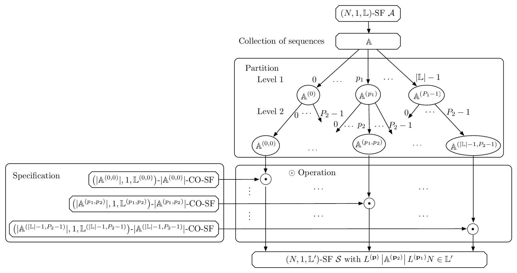
In general, for a given --CO-SF with , the following algorithm that is illustrated in Fig. 1 provides elongation of .
Algorithm 2
- 1.
Partition: Let be the set of all the sequences in . We consider a -level partition of such that, at the 1st level, the set is partitioned to SSs , , according to sequence lengths and, at the second level, each , an -SS, is further partitioned into -SSs .
- 2.
Specification: For each , let be an --CO-SF, the th SS of which has sequence length with a positive integer .
- 3.
Connection operation: Let and let be an -SF, , given by
(49) where we used the convention that specifies for some and specifies for some .
The following theorem is proved in Appendix III.
Theorem 3
If all the sequences in have the same energy for each , the -SF constructed by Algorithm 2 is an -CO-SF.
We note, for each subset at the st partition level, that its partition at the nd partition level can be arbitrary and that different partitions result in different -CO-SFs. For example, if we assume partition , , and with, respectively, , , and , and if we consider, correspondingly, -CO-SF, -CO-SF, and -CO-SF be , and , then the expression (49) gives another optimal --CO-SF
IV complete complementary codes
In this section, we study the least upper bound on the family size of a CCC as well as its generation and enlargement.
IV-A Upper bound and generation algorithm for CCC
As noted before, a CCC in a matrix form has a certain similarity to a unitary-like matrix. The following theorem is parallel to the fact that every matrix with the property for satisfies and is proved in Appendix IV (see also [53]).
Theorem 4
Every -CCC satisfies .
We say that an -CCC is optimal if . A unitary-like matrix is a special (or optimal) case of CCC satisfying and may be considered as an optimal CCC with length set .
We prove the following theorem in Appendix V.
Theorem 5
Given an --CO-SF , let be -SSs , . Then, for a unitary-like matrix , an -SF constructed as
| (51) |
is a CCC.
Example 6
From the --CO-SF in Example 3, we generate two SSs and . If we let , then we have an optimal -CCC
For a pair of length- vector and , we introduce entry-wise multiplication . Given a unitary matrix , if we consider the associated --CO-SF in Theorem 5, then and we have the following Corollary 1.
Corollary 1
Given a unitary-like matrix , the SF
| (57) |
is an -CCC.
Since the CCC given by Theorem 5 is constructed from an -CO-SF, it has the restriction that the sequence lengths are lower bounded by . To construct an -CCC with , we propose enlargement of a given CCC.
IV-B Enlargement of a CCC
For a length- vector and -SS , we introduce an operator22 2 This operation is defined by reference to the Kronecker product. to construct an -SS. Then, the next theorem gives a method to enlarge a given CCC.
Theorem 6
Given an -CCC and unitary-like matrices , , let be SSs given by
| (58) |
for and . Then, is an -CCC.
Proof:
The proof comes from the equalities
for and . ∎
Example 7
As an example, let and and enlarge the CCC given in Example 6 according to Theorem 6. Then, we have following optimal -CCC given in a matrix form
A CCC with is also possible by choosing large unitary-like matrices. For example, if we let , then Theorem 6 gives an -CCC.
V Family size, alphabet size, and sequence length
The CCC has attracted the attentions of numerous researchers because of its ideal correlation properties. Besides correlation properties, however, family size, alphabet size, and sequence length also play important roles in practical applications. In this section, we discuss these factors of the CCCs constructed by our algorithms.
V-A Family size
In Theorem 5, we gave a method to generate a CCC from an -CO-SF and unitary-like matrix . As a result, the generated CCC has, in matrix form, rows consisting of CSs and columns consisting of -CO-SFs, and hence the family size of the CCC and the size of each of the component CSs depend on the family size of the employed -CO-SFs. On the other hand, Theorem 4 shows that the family size of the CCC is upper bounded by the size of the component CSs. The two facts imply that the only way to increase the family size of the CCC is to increase the set size of the component CSs, and Theorem 6 gives a method to increase the set size of the component CSs. We note that the enlargement in Theorem 6 does not change the length set.
V-B Alphabet size
In Theorems 2, 3, 5, and 6, we only consider unitary-like matrices and the operations ‘connection’ and ‘multiplication’. Thus, if we can show the entries of the resultant sequences are bounded in a finite set, finite-alphabet construction becomes possible. Unitary-like matrices which allow this property are , which exists for any positive integer , and , which exists for with any positive integer . Employing in Corollary 1, we can derive a polyphase CCC with alphabet size while a binary CCC can be derived by employing in Corollary 1, where denotes the dyadic summation33 3 The dyadic summation of and is equal to if and only if their binary representations , , and satisfy , for all . of and . For example, employing in Corollary 1, we have a -CCC as
For an -CCC, in some applications as CCC-CDMA, it is expected for a higher spectral efficiency that the sum of correlations with adjacent sequence also vanishes as
| (78) |
for certain positive integer . Actually, if the SS generated by connecting sequences in each CS of a CCC becomes ZCZ-SS, then (78) holds. Hence, in [54], we called such a CCC a Z-connectable CCC (Z-CCC) and proved that the -CCCs derived by employing and in Corollary 1 are Z-CCC with and , respectively.
V-C Sequence length
Although each construction shown in this paper has a certain restriction on the length of resultant sequences, we can construct quite a large class of CCCs of variety of lengths by combining the proposed algorithms.
We first consider constructible sequence lengths for -CO-SFs. In our framework, one can generate an initial -CO-SF by Theorem 2 and extends the result using Theorem 3 iteratively. On the other hand, we may identify the collection of rows of a unitary-like matrix with an --CO-SF. Thus, we can show the following theorem by mathematical induction.
Theorem 7
Each sequence in the -CO-SFs constructed by Algorithm 1 and by iterative application of Algorithm 2 has a length equal to a product of integers which are not greater than . Conversely, given an integer which is decomposed into and factors not greater than , an -CO-SF whose length set includes can be constructed.
Proof:
For an , Algorithm 1 gives --CO-SFs with length set for subsets of . Therefore, and the first half of Theorem 7 is true for the -CO-SFs constructed by Algorithm 1.
Next, let us consider the lengths of -CO-SFs constructed by iterative application of Algorithm 2. We assume that we are given an --CO-SF with , at the beginning of Algorithm 2, and an --CO-SF with , at Specification step of Algorithm 2, where and are assumed to be decomposed into factors which are not greater than and factors which are not greater than , respectively. Then, the connection operation gives an SS with . Obviously, . Thus, given constituent -CO-SFs satisfying the first half of the theorem, Algorithm 2 gives an -CO-SF which also satisfies it.
Conversely, if a length can be decomposed by factors which are not greater than , the following algorithm yields an -CO-SF whose length set includes such a length. Assume the target length is for , then an -CO-SF whose length set includes can be constructed by Algorithm 1 from unitary-like matrices and and the resultant -CO-SF includes at least sequences with length . Hence, at Partition step of Algorithm 2, we have and may select such that . By specifying --CO-SF consisting of rows of unitary-like matrix at Specification step, Algorithm 2 yields at least length- sequences and, from , we may select such that at Partition step in the next iteration. By repeat the above process, we can construct an -CO-SF which includes length sequence(s). This completes the proof. ∎
Since and are only two integers not greater than , for instance, a -CO-SF whose length set includes can be constructed for any positive integer while a length- -CO-SF can not be constructed with our algorithms since includes a factor which is greater than . However, length- -CO-SF and other -CO-SFs which can not be constructed by our algorithm are not found at this moment.
Theorem 5 gives a mapping from a pair of an --CO-SF and a unitary-like matrix to an -CCC and lays a bridge between -CO-SFs and CCCs of the same length set . If we need an -CCC with large sequence lengths for a fixed , we can extend an -CO-SF by Algorithm 2 and apply the operation in Theorem 5. When we need to construct an -CCC with short sequence lengths, on the contrary, we construct -CCC based on -CO-SF with and enlarge the derived CCC by the operation in Theorem 6 to achieve the family size . As the results, we can construct CCCs whose lengths are independent with . Combining the result on the constructible lengths of -CO-SF, the CCCs constructed in our framework can be -CCCs whose length sets may contain length for arbitrary , where are any positive integers. Naturally, a question arises whether all CCCs are composed of -CO-SFs? Untill now, we have not found a CCC which is not composed of -CO-SFs, but its proof is not yet fully substantiated.
Existing construction algorithms for CCCs can be understood in our framework. For example, CCCs with length proposed by Suehiro and Hatori [5] can be generated for in Algorithm 1 and the lengthening method described in [5] can be obtained for in Algorithm 2. Han’s construction method in [37] can be obtained for with for all . The method given in [43] can be considered as application of Theorem 6 to a -CCC and for all .
VI Conclusion
In this paper, we proposed systematic and optimal constructions of -CO-SFs and CCCs. These constructions are realized by generation and extension methods and only unitary-like matrices are used. For any positive integers , , an -CCC with consisting of lengths for can be constructed by the use of presented methods and this form of CCC covers all the existing CCCs. In our framework, moreover, the alphabet size may be controlled by the appropriate selection of unitary-like matrices.
Appendix A Proof of Theorem 1
We consider an arbitrary --CO-SF with and let , . Next we introduce an matrix where denotes cyclicly right shift of . Then, the th entry of is given by
and, from the definition of -CO-SF and the identity (2), we have . On the other hand, the fact that means and hence means the bound .
Appendix B Proof of Theorem 2
Let and for . Because of Theorem 1, we only need to show that is an -CO-SF. Then, the correlation between , , and , , is given by
where we let and for simplicity.
Since consists of rows of and which are unitary-like matrices for all , the correlation is calculated as
This shows that is an -CO-SF and completes the proof.
Appendix C Proof of Theorem 3
For a given , we let , , and , and, for another , we introduce , , and in a similar manner. Moreover, we let .
We first note
for and, due to is chosen from an -CO-SF, we have
| (79) | |||||
On the other hand, the correlation between and can be expressed by
and, since is independent of for a given , by substituting , the correlation can be further calculated as
provided by and are chosen from a -CO-SF.
Appendix D Proof of Theorem 4
Let . Similarly to Appendix I, we extend each sequence in the CCC to length by and consider an matrix for . Then, we have and hence .
Appendix E Proof of Theorem 5
References
- [1] S. Verdú and S. Shamai (Shitz), “Spectral efficiency of CDMA with random spreading,” IEEE Trans. Inform. Theory, vol. 45, no. 2, pp. 622-640, Mar. 1999.
- [2] P. Fan and M. Darnell, Sequence Design for Communications Applications. New York: Wiley, 1999.
- [3] N. Suehiro and N. Kuroyanagi, “Multipath-tolerant binary signal design for approximately synchronized CDMA systems without co-channel interference using complete complementary codes,” in Proc. IEEE Global Telecommun. Conf. (GLOBECOM 1998), Nov. 1998, pp. 1356-1361.
- [4] N. Suehiro, N. Kuroyanagi, T. Imoto, and S. Matsufuji, “Very efficient frequency usage system using convolutional spread time signals based on complete complementary code,” in Proc. IEEE Int. Symp. Personal, Indoor and Mobile Radio Commun. (PIMRC’00), Sep. 2000, pp. 1567-1572.
- [5] N. Suehiro and M. Hatori, “-shift cross-orthogonal sequences,” IEEE Trans. Inform. Theory, vol. IT-34, no. 1, pp. 143-146, Jan. 1988.
- [6] S.-M. Tseng and M. R. Bell, “Asynchronous multicarrier DS-CDMA using mutually orthogonal complementary sets of sequences,” IEEE Trans. Commun., vol. 48, no. 1, pp. 53-59, Jan. 2000.
- [7] H.-H. Chen, H.-W. Chiu, and M. Guizani, “Orthogonal complementary codes for interference-free CDMA technologies,” IEEE Wireless Commun., vol. 13, no. 1, pp. 68-79, Feb. 2006.
- [8] C. Han, N. Suehiro, J. Chen, N. Kuroyanagi, and M. Nakamura, “Simulation of a parallel transmission system for multipath property to estimate pilot signals and additional chip-shifted information transmission signals,h in Proc. Int. Workshop Signal Design and Its Applications in Commun. (IWSDA’01), Sep. 2001, pp.107-116.
- [9] T. Kojima, A. Fujiwara, K. Yano, M. Aono, and N. Suehiro, “Comparison of the two signal design methods iin the CDMA systems using complete complementary codes,” IEICE Trans. Fundamentals, vol. E89-A, no. 9, pp. 2299-2306, Sep. 2006.
- [10] H.-H. Chen, J.-F. Yeh, and N. Suehiro, “A multicarrier CDMA architecture based on orthogonal complementary codes for new generations of wideband wireless communications,” IEEE Commun. Mag., vol. 39, no. 10, pp. 126-135, Oct. 2001.
- [11] H.-H. Chen, Y.-C. Yeh, Q. Bi, and A. Jamalipour, “On a MIMO-based open wireless architecture: space-time complementary coding,” IEEE Commun. Mag., vol. 45, no. 2, pp. 104-112, Feb. 2007.
- [12] L. Lu and V. K. Dubey, “Performance of a complete complementary code-based spread-time CDMA system in a fading channel,” IEEE Trans. Veh. Tech., vol. 57, no. 1, pp. 250-259, Jan. 2008.
- [13] N. Suehiro, “A signal design without co-channel interference for approximately synchronized CDMA systems,” IEEE J. Sel. Areas Commun., vol. 12, no. 5, pp. 837-841, June 1994.
- [14] R. Appuswamy and A. K. Chaturvedi, “A new framework for constructing mutually orthogonal complementary sets and ZCZ sequences,” IEEE Trans. Inform. Theory, vol. 52, no. 8, pp. 3817-3826, Aug. 2006.
- [15] C. Han, T. Hashimoto, and N. Suehiro, “Poly phase zero-correlation zone sequences based on complete complementary codes and DFT matrix,” in Proc. Int. Workshop Signal Design and Its Applications in Commun. (IWSDA’07), Sep. 2007, pp. 172-175.
- [16] C. Han, T. Hashimoto, and N. Suehiro, “A new construction method of zero-correlation zone sequences based on complete complementary codes,h IEICE Trans. Fundamentals, vol. E91-A, no.12, pp. 3698-3702, Dec. 2008.
- [17] N. S. Weerasinghe and T. Hashimoto, “Convolutional spreading CDMA and comparison with the DS-CDMA with RAKE receiver,” IEEE Trans. Commun., vol. 54, no. 11, pp. 1918-1922, Nov. 2006.
- [18] N. S. Weerasinghe, C. Han, and T. Hashimoto, “CS-CDMA/CP with ZCZ codes from an M-sequence and its performance for downlink transmission over a multipath fading channel,” IEICE Trans. Fundamentals, vol. E90-A, no. 6, pp. 1204-1213, June 2007.
- [19] S. E. El-Khamy, M. A. Mokhtar, and N. O. El-Ganainy, “New techniques for image change and motion detection based on complete complementary code arrays,” in Proc. Radio Science Conf. (NRSC 2004), Mar. 2004, pp. C35-1-8.
- [20] S. E. El-Khamy, N. O. El-Ganainy, and M. A. Mokhtar, “The twin image watermarking algorithm (TIWA): A new techniques for single and multi-message watermarking based on optimum complete complementary codes,” in Proc. Int. Conf. Comp. as a Tool (EUROCON 2005), Nov. 2005, pp. 939-942.
- [21] T. Detert, W. Haak, and I. Martoyo, “Complete complementary codes applied to UTRA FDD asynchronous uplink,” in Proc. IEEE Mediterranean Electrotechnical Conf. (MELECON 2004), May 2004, pp. 441-444.
- [22] J. Liu, G. Kang, S. Lu, and P. Zhang, “Preamble design based on complete complementary sets for random access in MIMO-OFDM systems,” in Proc. Wireless Commun. and Networking Conf. (WCNC 2007), Mar. 2007, pp. 858-862.
- [23] S. Ozgur and D. B. Williams, “Temporal partition particle filtering for multiuser detectors with mutually orthogonal sequences,” in Proc. IEEE Int. Conf. Acoustics, Speech, and Signal Processing (ICASSP 2005), Mar. 2005, pp. iii/1033-iii/1036.
- [24] M. J. E. Golay, “Complementary series,” IRE Trans. Inform. Theory, vol. IT-7, no. 2, pp. 82-87, Apr. 1961.
- [25] R. Turyn, “Ambiguity function of complementary sequences,” IEEE Trans. Inform. Theory, vol. IT-9, no. 1, pp. 46-47, Jan. 1963.
- [26] Y. Taki, H. Miyakawa, M. Hatori, and S. Namba, “Even-shift orthogonal sequences,” IEEE Trans. Inform. Theory, vol. IT-15, no. 2, pp. 295-300, Mar. 1969.
- [27] C. C. Tseng, and C. L. Liu, “Complementary sets of sequences,” IEEE Trans. Inform. Theory, vol. IT-18, no. 5, pp. 644-652, Sep. 1972.
- [28] R. Sivaswamy, “Multi-phase complementray codes,” IEEE Trans. Inform. Theory, vol. IT-24, no. 5, pp. 546-552, Sep. 1978.
- [29] R. L. Frank, “Poly-phase complementary codes,” IEEE Trans. Inform. Theory, vol. IT-26, no. 6, pp. 641-647, Nov. 1980.
- [30] J. A. Davis and J. Jedwab, “Peak-to-mean power control in OFDM, Golay complementary sequences, and Reed-Muller codes,” IEEE Trans. Inform. Theory, vol. 45, no. 7, pp. 2397-2417, Nov. 1999.
- [31] R. V. Nee and R. Prasad, OFDM for Wireless Multimedia Communications. Artech House Publishers, 2000.
- [32] C. Röing and V. Tarokh, “A construction of OFDM 16-QAM sequences having low peak powers,” IEEE Trans. Inform. Theory, vol. 47, no. 5, pp. 2091-2094, July 2001.
- [33] B. Tarokh and H. R. Sadjadpour, “Construction of OFDM -QAM sequences with low peak-to-average power ratio,” IEEE Trans. Commun., vol. 51, no. 1, pp. 25-28, Jan. 2003.
- [34] H. Lee and S. H. Golomb, “A new construction of 64-QAM Golay complementary sequences,” IEEE Trans. Inform. Theory, vol. 52, no. 4, pp. 1663-1670, Apr. 2006.
- [35] Y. Li and W. B. Chu, “More Golay sequences,” IEEE Trans. Inform. Theory, vol. 51, no. 3, pp. 1141-1145, Mar. 2005.
- [36] F. Fiedler and J. Jedwab, “How do more Golay sequences arise?” IEEE Trans. Inform. Theory, vol. 52, no. 9, pp. 3220-3232, July 2006.
- [37] C. Han, N. Suehiro, and T. Imoto, “A generation method for constructing complete complementary sequences”, The World Scientific and Engineering Academy and Society (WSEAS) Trans. Commun., vol. 3, no. 2, pp. 530-534, Apr. 2004.
- [38] C. Han and N. Suehiro, “A generation method for constructing complete-complementary sequences,” in Proceedings of the Joint IST Workshop on Mobile Future and Symposium on Trends in Communications (Sympotic’04), Oct. 24-26, 2004, pp. 70-73.
- [39] R. S. Raja Durai, N. Suehiro, and C. Han, “Complete complementary sequences of different length,” IEICE Trans. Fundamentals, vol. E90-A, no. 7, pp. 1428-1431, July 2007.
- [40] X. Huang and Y. Li, “Scalable complete complementary sets of sequences”, in Proc. IEEE Globe Telecommun. Conf. (GLOBECOM 2002), Nov. 2002, pp.1056-1060.
- [41] L. Lu and V. K. Dubey, “Extended orthogonal polyphase codes for multicarrier CDMA system,” IEEE Commun. Lett., vol. 8, no. 12, pp. 700-702, Dec. 2004.
- [42] C. De Marziani, J. Urena, A. Hernandez, M. Mazo, F. J. Alvarez, J. J. Garcia, and P. Donato, “Modular architecture for efficient generation and correlation of complementary set of sequences,” IEEE Trans. Signal Processing, vol. 55, no. 5, pp. 2323-2337, May 2007.
- [43] X. Yang, Y. Mo, D. Li, and M. Bian, “New complete complementary codes and their analysis,” in Proc. IEEE Globe Telecommun. Conf. (GLOBECOM 2007), Nov. 2007, pp. 3899-3904.
- [44] W. Di and P. Spasojević, “Complementary set matrices satisfying a column correlation constraint,” IEEE Trans. Inform. Theory, vol. 54, no. 7, pp. 3330-3339, 2008.
- [45] C. Y. Chen, C. H. Wang, and C. C. Chao, “Complete complementary codes and generalized reed-muller codes,” IEEE Commun. Lett., vol. 12, no. 11, pp. 849-851, Nov. 2008.
- [46] H. Torii, N. Suehiro, and M. Nakamura, “General construction of periodic complete complementary codes composed of expanded modulatable orthogonal sequences,” in Proc. IEEE Symp. Computers and Commun. (ISCC’00), July 2000, pp. 738-743.
- [47] H. Torii, M. Nakamura, and N. Suehiro, “Generalized method for constructing modulatable periodic complete complementary codes,” in Proc. IEEE Workshop on Signal Processing Advances in Wireless Commun. (SPAWC 2001), Mar. 2001, pp. 259-262.
- [48] P. Farkas and M. Turcsany, “Two-dimensional orthogonal complete complementary codes,” in Proc. the Joint IST Workshop on Mobile Future and Symp. on Trends in Commun. (Sympotic’03), Oct. 2003, pp. 21-24.
- [49] M. Turcsany and P. Farkas, “Three-dimensional orthogonal complete-complementary codes,” in Proc. Joint IST Workshop on Mobile Future and Symp. on Trends in Commun. (Sympotic’04), Oct. 2004, pp. 98-101.
- [50] C. Zhang, X. Lin, and M. Hatori, “Two dimensioan combined complementary sequence and its application in multi-carrier CDMA,” IEICE Trans. Commun., vol. E88-B, no. 2, pp. 478-486, Feb. 2005.
- [51] R. S. Raja Durai and N. Suehiro, “Higher dimensional complete-complementary sequences: A generalized approach,” in Proc. Int. Symp. on Inform. Theory and its Applications (ISITA 2006), Oct. 2006, pp. 928-933.
- [52] C. Han, N. Suehiro, and T. Hashimoto, “Least upper bound of family number of -shift cross-orthogonal sequences,” (in Japanese) IEICE Trans. Fundamentals, vol. J90-A, no.3, pp. 248-251, Mar. 2007.
- [53] C. Han and N. Suehiro, “Upper bound of number of families in a periodic complete complementary sequence set and a complete complementary set,” (in Japanese) IEICE Trans. Fundamentals, vol. J88-A, no. 9, pp. 1071-1073, Sep. 2005.
- [54] C. Han and T. Hashimoto, “-connecteble complete complementary code and its application in CDMA,” in Proc. Int. Symp. Inform. Theory (ISIT2009), June 2009, pp.438-422.