Instability of Bose-Einstein condensates in tilted lattices with time-periodical modulation

Since Bose-Einstein condensation (BEC) of dilute gases of alkali atoms was realized in 1995 [1, 2, 3], much attention has been paid to the ultracold atomic systems in various configurations, such as optical lattices which are formed by counter-propagating laser beams. Due to the flexibility of the system, the famous Mott-insulator-Superfluid transition of BECs in optical lattices has been observed and studied [4, 5]. Dynamically, there are also many interesting phenomena, such as the resonant tunneling [6]. In the limit of vanishing particle interactions, ${\it e.g.}$, in dilute bosonic gases, the system may exhibit Bloch oscillation [7, 8], similar to the behavior of single electron in the crystalline field of solids. Other than the energetic instability [9] induced by the non-zero temperature, the nonlinear scattering process may also cause the dynamical instability [10] damping the oscillation behavior [11].

Dynamical stability, which describes whether the system remains stable or not during its time evolution, is our concern in this paper. We are interested in the dynamical response of BECs in modulated optical lattices. We notice that dynamical stability of BECs system in an optical lattice modulated by a time-periodic potential has been investigated in both experiment [12] and theory [13]. Also, dynamical stability of the condensates in tilted optical lattices considering the effect of a constant acceleration force has attracted many people’s attention [14, 15]. Recently BECs in tilted time-periodically modulated lattices formed by both a time-periodic modulation potential and a constant acceleration force was realized experimentally [16]. We focus on the dynamical stability of the above system to which few attention has been paid before, and aim to find out the influence of the interparticle interactions.

The structure of this paper is organized as follows. In Sec. II we describe our modulated optical lattice system with modified Bose-Hubbard Hamiltonian [17, 18]. In mean-field approximation we derive the time-evolution equations and obtain the explicit solutions. In order to determine the dynamical stability of the system, we adopt an ansatz of the time-evolution operator [13, 14]. Upon Floquet theorem, the quasienergy analysis, which is strongly related to the dynamical stability, is given in Sec. III. Based on the ratio of the acceleration force to the modulation frequency, two specific cases, integer and non-integer resonances, are considered. We also discuss the main features of dynamical stability for both two cases in Sec. IV. A summary with brief discussion is given in Sec. V.

We consider ultracold bosonic gases on an one-dimensional optical lattice modulated by both a time-periodic potential and a constant external acceleration force simultaneously. To model such a system, we need to include the external modulation terms in the typical Bose-Hubbard Hamiltonian (BHH), i.e.,

Here $\hat{a}_{m}~(\hat{a}^{{\dagger}}_{m})$ annihilates (creates) a boson on the $m$th lattice site, and $\hat{n}_{m}=\hat{a}^{\dagger}_{m}\hat{a}_{m}$ is the particle number operator correspondingly. $J$ describes the hopping strength between adjacent sites which are indicated by the subscript $\langle m,n\rangle$. $U$ refers to the on-site interaction between atoms. $K$ and $\omega$ denote the amplitude and frequency of the time-periodic modulation potential, while $d$ stands for the constant acceleration force.

The dynamical properties of our system can be obtained by studying the Heisenberg equations of motion for $\hat{a}_{m}$. Provided that the particle number of atoms on each site is large enough, we can safely adopt the mean-field approximation (MFA) to replace these operators with their expectation values, e.g., $\alpha_{m}=\langle\hat{a}_{m}\rangle/\sqrt{N_{L}}$, where $N_{L}$ is the average number of atoms per site. Then the time-evolution equations for $\alpha_{m}$ are expressed as

where the natural unit $\hbar=1$ is taken and $g=N_{L}U$ denotes the normalized atomic interaction. Eqs. (2) are also regarded as discretized Gross-Pitaevskii (GP) equations. Additionally, the particle number conservation $\sum_{m}\hat{a}^{\dagger}_{m}\hat{a}_{m}=N$ gives $\sum_{m}|\alpha_{m}|^{2}=L$, where $N$ and $L$ are the total numbers of atoms and optical lattice sites, respectively, and their ratio is $N_{L}$, ${\it i.e.}$, $N_{L}=N/L$.

In the interaction-free case, i.e., $g=0$, Eqs. (2) describe the single-particle dynamics whose analytical solutions can be explicitly derived through the gauge transformation [15]

then Eqs. (2) become

where $D(t)=dt+K/{\omega}\sin(\omega t)$. Because the translation symmetry is retrieved back in the above equation, we can impose the spatial periodic boundary conditions, ${\it i.e.}$, $\tilde{\alpha}_{m}(t)=\tilde{\alpha}_{L+m}(t)$. The corresponding semi-classical Hamiltonian now reads

The Bloch-wave representation is desirable in order to obtain the solutions for $\tilde{\alpha}_{m}$,

where $k=2\pi n/L$ is the quasimomentum ($-\pi\leq k<\pi$), $n=0,\pm 1,\ldots,\pm(L-1)/2$ for odd $L$, while $n=0,\pm 1,\ldots,\pm L/2$ for even $L$. Then the evolution equations of $b_{k}$ take the following simple form

whose solutions can be explicitly expressed as

Here the factor $b_{k}(0)$ is the integral constant, and $S(t)$ and $C(t)$ are defined as

where $\mathcal{J}_{n}$ denotes the $n$th ordinary Bessel function.

The analytical solutions $\alpha_{m}$ for $g=0$ can be directly obtained through the inverse Fourier transformation. They are the starting points to derive the trial solutions for $g\neq 0$ case. Specifically, we are concerned about $b_{k}(0)=\delta_{k,p}$ case, which can simplify the final expressions of solutions of Eqs. (2) as

Note that the solutions are applicable for $L\rightarrow\infty$ in which the boundary conditions make no difference.

To explore the dynamical stability of the system, we assume small fluctuations around the stationary solutions following the usual ansatz [13, 14], i.e., $\alpha_{m}(t)=\alpha^{0}_{m}(t)+\delta\alpha_{m}(t)$, where $\alpha^{0}_{m}(t)$ take the expressions as Eqs. (11). The fluctuations can be expressed as

Here $q$ is the momentum of the excitation relative to the condensate. Substituting the trial solutions into Eqs. (2), we obtain the Bogoliubov-de Gennes (BdG) equations for the quasiparticle excitations $u(t)$ and $v(t)$,

where the elements of the matrix $\mathcal{M}(q,t)$ are given by

Note that the matrix $\mathcal{M}(q,t)$ is also time-periodic with the periodicity $T$ being the lowest common multiple of $2\pi/\omega$ and $2\pi/d$.

It will be convenient to introduce the evolution operator $U(t)$ in order to characterize the evolution of $u(t)$ and $v(t)$, ${\it i.e.}$, $(u(t),v(t))^{T}=U(t)(u(0),v(0))^{T}$. Thus, the dynamical behavior $U$ is governed by

Using the $2\times 2$ unit matrix as the initial data, we numerically solve Eq. (14) over period $T$. According to the Floquet theorem, the eigenvalues $\lambda_{i}$ of $U(T)$ correspond to the excitation quasienergies $\varepsilon_{i}$ via $\lambda_{i}=\exp[-i\varepsilon_{i}T]$ ($i=1,2$). The dynamical stability of the system is specified by the fact that both the quasienergies $\varepsilon_{i}$ have no imaginary components, ${\it i.e.}$, $|\lambda_{i}|=1$. If so for all values of $q$, then the solution is stable. Otherwise, the system may collapse. The analysis of those features can help us to map out the stability diagrams of the system in the parameter space of $g/\omega$ and $K/\omega$ which are shown in Sec. IV.

As stated above, quasienergies are tightly related to the dynamical stability. Since the period of the time-periodic evolution matrix in Eqs. (4) is $T$, the Floquet theorem enables us to write the solution in the form of $\exp[-i\varepsilon t]\psi(t)$, where $\varepsilon$ corresponds to the quasienergy of the system and $\psi(t)$ corresponds to the Floquet state which shares the same period $T$. In order to obtain the quasienergies, we pick out all terms which are not $T$-periodic from $\alpha_{m}(t)$ [13]. Note that $g=n\omega+g^{\prime}$ where $n$ is a positive integer to ensure $0\leq g^{\prime}<\omega$. Considering the possible divergence in the denominators of summations in $S(t)$ and $C(t)$, we analyze, separately, the cases of $l=d/\omega$ being integer and non-integer.

For integer $l$, in the limit of $d\rightarrow l\omega$, both $\exp[\sin(-l\omega+d)t/(-l\omega+d)]\rightarrow t$ and $\exp[-ig^{\prime}t]$ are not $T$-periodic, then we have the quasienergies expressed as

The situation of $d=0$ has already been studied in Ref. [13], so here we discuss more general case $d\neq 0$. Throughout our paper, $J$ is set to be the unit. For example, we show the quasienergy spectrum for $d=\omega$ ($l=1$) and $d=2\omega$ ($l=2$) in Fig. 1(a) and 1(b), respectively. The spectrum is obtained by the fundamental matrix method, which requires the diagonalization of $\vec{\alpha}(0)^{T}\vec{\alpha}(T)$ where $\vec{\alpha}(t)=\{\alpha_{1}(t),\alpha_{2}(t),\ldots,\alpha_{L}(t)\}$. As $L\rightarrow\infty$, the results match the analytical expressions (15) perfectly. Another numerical way to obtain the quasienergies is to evolve the time-evolution operator of $\vec{\alpha}(t)$ directly and diagonalize it, which yields the same results. It is obviously observed from Fig. 1(a) and 1(b) that the spectrum is wholly displaced by the amount of $g^{\prime}$ , as stated above. And the collapse points of the spectrum correspond to the zeroes of $\mathcal{J}_{-l}(K/\omega)$, which manifests the phenomenon of the “coherent destruction of tunneling” (CDT) effect.

For non-integer $l$, the case is much simpler since all terms in $\alpha_{m}(t)$ have the periodicity $T$ except $\exp[-ig^{\prime}t]$. One can conclude that the quasienergies of the system are $\varepsilon(p)=g^{\prime}$, independent of the value of $K/\omega$. Our numerical calculations further confirm our analysis.

We are interested in the dynamical stability of the system around the ground state, ${\it i.e.}$, $p=0$. To determine the critical interaction $g_{c}$ beyond which the system becomes unstable, we increase the value of $g$ from zero gradually for each $K/\omega$ until the unstable region is reached. Then we are able to plot the boundary between stable and unstable regions in the parameter space of $g/\omega$ and $K/\omega$.

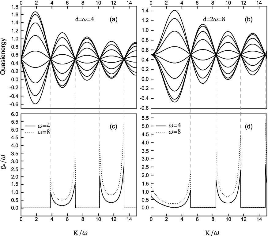
Since Eq. (14) can be solved analytically when $g=0$, it is easy to find that the excitation quasienergies are all real such that the system is always stable regardless of the value of $K/\omega$. As $g$ increases, the unstable regions emerge. We observe different stability diagrams for integer and non-integer $l$.

For the case of integer $l$, we plot the stability diagrams for $l=1$ and $l=2$ in Fig. 1(c) and 1(d), respectively. It is clear that the dependence of $g_{\mathrm{c}}$ on $K/\omega$ shows two kinds of alternative behaviors between plateau and upward concave shapes. We notice that the separations between the two behaviors appear at the collapse points of the quasienergy spectrum, also the zeros of $\mathcal{J}_{-l}(K/\omega)$. From Eq. (15) we may define the effective hopping strength $J_{\mathrm{eff}}(K/\omega)=J\mathcal{J}_{-l}(K/\omega)$, while the flat critical interaction regions ($g_{\mathrm{c}}\rightarrow 0$) correspond to the negative $J_{\mathrm{eff}}$. The instability can be understood as the effect of attractive interactions [19] for positive $J_{\mathrm{eff}}$ due to the symmetry of the system Hamiltonian [20]. When $J_{\mathrm{eff}}(K/\omega)=0$, CDT happens, freezing the dynamics of the system, thus insuring the stability. $g_{\mathrm{c}}$ peaks around these critical points.

Comparing Fig. 1(c) and 1(d) we notice a seemingly natural, however, interesting phenomenon. When $l$ is a positive odd integer, in the limit of infinite small, however nonzero $K/\omega\rightarrow 0$, the system is always unstable for any infinite small value of interaction, i.e., $g_{\mathrm{c}}\rightarrow 0$. The specific choices of $l$ insure the emergence of the phenomenon which has not been observed in the case of $l=0$ [13].

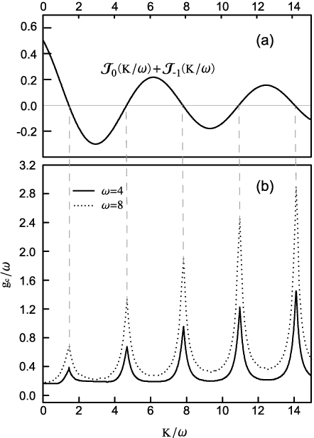
For the case of non-integer $l$, the analysis is totally different, of which we start with half-integer $l$ case. As an example, we plot the stability diagram for $l=0.5$ in Fig. 2(b). Since the quasienergies for non-integer $l$ are constant independent of $K/\omega$, no correspondence between the quasienergies and $g_{\mathrm{c}}$ peaks is observed, as expected. In order to determine the positions of $g_{\mathrm{c}}$ peaks approximately, we have to resort to the expression of $\alpha_{m}(t)$. Since the summations appear in the exponent of Eq. (11), as $|n+l|$ increases, the contribution from the $n$-th term reduces rapidly, if the high modulation frequency limit is assumed, i.e., $\omega\gg 1/J$ [21]. The dominant terms would be those with the smallest values of $|n+l|$. As an example, for $l=0.5$, the dominant contributions to $\alpha_{m}(t)$ would come from $\mathcal{J}_{0}(K/\omega)+\mathcal{J}_{-1}(K/\omega)$ which is plotted in Fig. 2(a). The correspondence between the zeros of Bessel functions and $g_{\mathrm{c}}$ peaks is observed, confirming our analysis. As stated before, the dynamics of the system is frozen at the zeros of Bessel functions, indicating the appearance of stable regions, where $g_{\mathrm{c}}$ peaks with greatest probability. We also notice the whole displacement of $g_{c}$ whose value depends on $d$. In Fig. 3 we plot the behaviors of dynamical stability around integer and half-integer $l$, compared with which the crossover between them shows no explicit dependence of $g_{\mathrm{c}}$ on the values of $K/\omega$. We may interpret the behavior as the counterbalance of different Bessel functions. Also from Fig. 3, we can find the same dependence of $g_{\mathrm{c}}$ on $d$ as found in Ref. [15] without time-periodical modulation, ${\it i.e.}$, $K/\omega=0$.

Additionally, for both integer and non-integer $l$, we find that the bigger value of $\omega$ favors the high modulation frequency limit, also enhances the dynamical stability of the system as shown in Fig. 1(c), 1(d) and Fig. 2(b).

We considered the system of BECs in one-dimensional tilted time-periodically modulated lattices. The ratio $l$ of the acceleration force $d$ to the modulation frequency $\omega$ is defined to help dividing our analysis into integer and non-integer resonances. Due to the time-periodicity of the system Hamiltonian, we gave the explicit expressions of quasienergies for both cases referring to integer and non-integer resonances by making use of Floquet theorem. For integer $l$, the quasienergy spectrum shows its correspondence to the Bessel function $\mathcal{J}_{-l}(K/\omega)$ whose zeros correspond to the collapse points of the spectrum, indicating the appearance of CDT. However, for non-integer $l$, no dependence of the quasienergies on $K/\omega$ is found.

We investigated the dynamical stability of the system by characterizing it in the parameter space of the interaction strength and the modulation amplitude. For integer $l$, we observed two alternate behaviors of the dependence of the critical interaction strength $g_{\mathrm{c}}$ on $K/\omega$: plateau ($g_{\mathrm{c}}\rightarrow 0$) and upward concave. The complete instability in horizontally flat regions is brought out by the negative effective tunneling strength. The separations between the two kinds of regions correspond to the zeros of Bessel Function $\mathcal{J}_{-l}(K/\omega)$. We also noticed an interesting phenomenon when $l$ is a positive odd integer. In such case, the system is always unstable in the limit of $K/\omega\rightarrow 0$ corresponding to the infinite small, however, nonzero modulation potential. Among non-integer resonances, we observed that $g_{\mathrm{c}}$ peaks are centered around half-integer $l$ for which the completely unstable regions disappear. Also the whole displacement of $g_{\mathrm{c}}(K/\omega)$ emerges whose value is dependent on $d$. The positions of $g_{\mathrm{c}}$ peaks in the direction of $K/\omega$ are determined approximately in the high modulation frequency limit. Compared with integer and half-integer resonances, the crossovers between them show no explicit dependence of $g_{\mathrm{c}}$ on the modulation amplitude. Since dynamical stability is experimentally observable, these features are expected to be confirmed in experiment.

The work is supported by NSFC Grant No. 10874149 and partially by PCSIRT Grant No. IRT0754.

References

- [1] M. H. Anderson, J. R. Ensher, M. R. Matthews, C. E. Wieman, E. A. Cornell, Science 269, 198 (1995).
- [2] C. C. Bradley, C. A. Sackett, J. J. Tollett, and R. G. Hulet, Phys. Rev. Lett. 75, 1687 (1995).
- [3] K. B. Davis, M. -O. Mewes, M. R. Andrews, N. J. van Druten, D. S. Durfee, D. M. Kurn, and W. Ketterle, Phys. Rev. Lett. 75, 3969 (1995).
- [4] M. Greiner, O. Mandel, T. Esslinger, T. W. Hänsch, and I. Bloch, Nature (London) 415, 39 (2002).
- [5] C. E. Creffield and T. S. Monteiro, Phys. Rev. Lett. 96, 210403 (2006).
- [6] C. Sias, A. Zenesini, H. Lignier, S. Wimberger, D. Ciampini, O. Morsch, and E. Arimondo, Phys. Rev. Lett. 98, 120403 (2007).
- [7] O. Morsch, J. H. Müller, M. Cristiani, D. Ciampini, and E. Arimondo, Phys. Rev. Lett. 87, 140402 (2001).
- [8] A. Eckardt, M. Holthaus, H. Lignier, A. Zenesini, D. Ciampini, O. Morsch, and E. Arimondo, Phys. Rev. A 79, 013611 (2009).
- [9] B. Wu and Q. Niu, Phys. Rev. A 64, 061603(R) (2001).
- [10] B. Wu and Q. Niu, New J. Phys. 5, 104 (2003).
- [11] L. Fallani, L. De Sarlo, J. E. Lye, M. Modugno, R. Saers, C. Fort, and M. Inguscio, Phys. Rev. Lett. 93, 140406 (2004).
- [12] H. Lignier, C. Sias, D. Ciampini, Y. Singh, A. Zenesini, O. Morsch, and E. Arimondo, Phys. Rev. Lett. 99, 220403 (2007).
- [13] C. E. Creffield, Phys. Rev. A 79, 063612 (2009).
- [14] Y. Zheng, M. Kostrun, and J. Javanainen, Phys. Rev. Lett. 93, 230401 (2004).
- [15] A. R. Kolovsky, H. J. Korsch and E. M. Graefe, Phys. Rev. A 80, 023617 (2009).
- [16] C. Sias, H. Lignier, Y. P. Singh, A. Zenesini, D. Ciampini, O. Morsch, and E. Arimondo, Phys. Rev. Lett. 100, 040404 (2008).
- [17] A. Eckardt, T. Jinasundera, C. Weiss, and M. Holthaus, Phys. Rev. Lett. 95, 200401 (2005).
- [18] A. R. Kolovsky and H. J. Korsch, e-print arXiv:0912.2587.
- [19] J. C. Bronski, L. D. Carr, R. Carretero-Gonzlez, B. Deconinck, J. N. Kutz and K. Promislow, Phys. Rev. E 64, 056615 (2001).
- [20] C. J. Myatt, E. A. Burt, R. W. Ghrist, E. A. Cornell and C. E. Wieman, Phys. Rev. Lett. 78, 586 (1997).
- [21] C. E. Creffield, Phys. Rev. B 67, 165301 (2003).