Nature of the spin-glass phase at experimental length scales

We consider the $D=3$ Edwards-Anderson model [28, 29]. Our dynamical variables are Ising spins $s_{\bi x}\!=\!\pm 1$, which are placed on the nodes, $\bi x$, of a cubic lattice of linear size $L$, containing $V=L^{3}$ sites, and with periodic boundary conditions. Their interaction is restricted to lattice nearest neighbours and is given by the Hamiltonian:

Note that the couplings $J_{\bi x,\bi y}$ in the Hamiltonian are themselves stochastic variables: they take the values $\pm 1$ with $50\%$ probability. The coupling constants attached to different lattice links are statistically independent. The physical motivation for working with a random Hamiltonian is modelling the effects of impurities in a magnetic alloy.

We shall consider the quenched approximation: in the time scale relevant to the spin dynamics, the impurities can be regarded as static. Hence, we will not allow for any back-reaction of the spins over the coupling constants. A given realisation of the $\{J_{\bi x,\bi y}\}$ (a sample, from now on), will be fixed from the start and considered non-dynamical [1].

A random Hamiltonian implies a double averaging procedure. For any observable $O$ (an arbitrary function of the spins and the coupling constants), we shall first compute the thermal average $\langle O\rangle$ using the Boltzmann weight at temperature $T$ for the Hamiltonian (1). The average over the coupling constants distribution, $\overline{\langle O\rangle}\,,$ is only taken afterwards. We will refer sometimes to the second averaging, $\overline{(\cdot\cdot\cdot)}$, as disorder average.

The reader will notice that the disorder average induces a non-dynamical gauge symmetry [30]. Let us choose a random sign per site $\epsilon_{\bi x}=\pm 1\,$. Hence, the energy (1) is invariant under the transformation

Since the gauge-transformed couplings $\epsilon_{\bi x}\epsilon_{\bi y}J_{{\bi x},{\bi y}}$ are just as probable as the original ones, the quenched mean value of $\overline{\langle O(\{s_{\bi x}\})\rangle}$ is identical to that of its gauge average $\sum_{\{\epsilon_{\bi x}=\pm 1\}}\overline{\langle O(\{\epsilon_{\bi x}s_{\bi x}\})\rangle}/2^{L^{D}}\,,$ which typically is an uninteresting constant value. We show in section 2.2 how to overcome this problem.

We remark as well that the Hamiltonian (1) also has a global $\mathbf{Z}_{2}$ symmetry (if all spins are simultaneously reversed $s_{\bi x}\to-s_{\bi x}$ the energy is unchanged), corresponding to time-reversal symmetry. This symmetry gets spontaneously broken in three dimensions upon lowering the temperature at the SG transition at $T_{\mathrm{c}}=1.109(10)$ [31, 32].

We need observables that remain invariant under the transformation (2). The Hamiltonian (1) provides, of course, a first example. To make further progress we consider real replicas $\{s_{\bi x}^{(1)}\},\{s_{\bi x}^{(2)}\}$, copies of the system that evolve under the same set of couplings $\{J_{{\bi x},{\bi y}}\}$ but are otherwise statistically uncorrelated.¹¹ 1 For the thermal average of any observable depending on a single spin configuration, $O(\{s_{\bi x}^{(1)}\})$, we have $\bigl\langle O(\{s_{\bi x}^{(1)}\})\bigr\rangle^{2}=\bigl\langle O(\{s_{\bi x}^{(1)}\})\,O(\{s_{\bi x}^{(2)}\})\bigr\rangle$.

Using them we form the overlap field:

which is obviously invariant under (2).

The Edwards-Anderson order parameter, the spin overlap, is the spatial average of the overlap field:

In particular, it yields the (non-connected) spin-glass susceptibility

that diverges at $T_{\mathrm{c}}$ with the critical exponent $\gamma$. For all $T<T_{\mathrm{c}}$, one expects $\chi_{\mathrm{NC}}={\cal O}(V)\,$. We shall also consider the Binder ratio

In particular, for all $T>T_{c}$, the fluctuations of $q$ are expected to be Gaussian in the large-$L$ limit, hence $\lim_{L\to\infty}B=3$, $(T>T_{\mathrm{c}})$. Its behaviour in the low-temperature phase is controversial. For a disguised ferromagnet picture one expects $B$ to approach $1$ in the limit of large lattices. On the other hand, for an RSB system one expects $1<B<3$ in the SG phase ($T<T_{\mathrm{c}}$). We recall also that one may consider as well the overlap computed in small boxes, in order to avoid the effect of the interphases (physical results are equivalent to those obtained with the standard overlap [33]).

A great deal of attention will be devoted to the probability density function (pdf) of the overlap

Note that, in a finite system, the pdf is not smooth, but composed of $N+1$ Dirac deltas at $q=-1,-\frac{N-2}{N},\ldots,\frac{N-2}{N},1$. Here, we have solved this problem by a convolution of the comb-like pdf (7) with a Gaussian of width $1/\sqrt{V}$, ${\cal G}_{V}(x)=\sqrt{\frac{V}{2\pi}}\mathrm{exp}[-V\frac{x^{2}}{2}]\,$:

In this way, we basically add the contribution of ${\cal O}(\sqrt{V})$ microscopic values of $q$, belonging to an interval of width $\sim 1/\sqrt{V}$ [34]. Note, however, that eqs. (5,6) are computed out of moments of $\tilde{P}(q)$, rather than of $P(q)$.

The Edwards-Anderson order parameter $q_{\mathrm{EA}}$ vanishes for all $T\geq T_{\mathrm{c}}$. Below $T_{\mathrm{c}}$, in a droplet system, $P(q)$ collapses in the large-$L$ limit in a pair of Dirac delta functions of equal weight, centred at $q=\pm q_{\mathrm{EA}}$. In an RSB system, $P(q)$ contains as well a pair of delta functions at $q_{\mathrm{EA}}$, but it also has a continuous piece, non-vanishing for every $q$ such that $-q_{\mathrm{EA}}<q<q_{\mathrm{EA}}$. This is the origin of the differences in the predictions that both theories make for $B$ in the low-temperature phase.

We will find it useful to consider as well conditional expectation values at fixed $q$. Let $O$ be an arbitrary function of the spins. We define its conditional expectation

Of course, one may easily recover standard expectation values from $\mathrm{E}(O|q)$:

Strictly speaking, the integration limits should be $\pm\infty$. However, truncating the integral to $-1<q<1$, the error is exponentially small in $L^{D/2}$ (yet, for $L\!=\!8$ and $12$ we had to extend the limits beyond $\pm 1$).

We can also define the conditional variances as

where we have the identity

The overlap correlation function is

$C_{4}(\bi r)$ decays to zero for large $\bi r$ only for $T>T_{\mathrm{c}}$. Thus we have considered as well conditional correlation functions, recall eq. (9):

Eq. (10) allows us to recover $C_{4}(\bi r)$ from $C_{4}(\bi r|q)$.

The two main theoretical pictures for the SG phase, the droplet and RSB pictures, dramatically differ on their predictions for $C_{4}(\bi r|q)$. Let us discuss them in detail:

• •

  In the RSB picture, the connected correlation functions tend to zero at large $\bi r$. For all $q\in[-q_{\mathrm{EA}},q_{\mathrm{EA}}]$ we expect the asymptotic behaviour

  $$C_{4}(\bi r|q)\sim q^{2}+\frac{A_{q}}{r^{\theta(q)}}+\ldots\,,$$

  (15)

  where the dots stand for scaling corrections, subleading in the limit of large $r$. The exponent $\theta(q)$ in eq. (15) has been computed for $D$ larger than the upper critical dimension $D_{\mathrm{u}}=6$: [35, 36]

  	$\displaystyle\theta(q=0)$	$\displaystyle=$	$\displaystyle D-4\,,$		(16)
  	$\displaystyle\theta(0<|q|<q_{\mathrm{EA}})$	$\displaystyle=$	$\displaystyle D-3\,,$		(17)
  	$\displaystyle\theta(|q|=q_{\mathrm{EA}})$	$\displaystyle=$	$\displaystyle D-2\,.$		(18)

  These mean-field results for $\theta(q)$ become inconsistent for $D<4$ [the correlations should decrease for large $r$, implying $\theta(q)>0$, recall eq. (15)]. An expansion in $\epsilon=6-D$ suggests that $\theta(q)$ will renormalise [37]. Note as well that, at least for large $D$, $\theta(q)$ is discontinuous at $q=0$. However, we remark that there are no compelling theoretical arguments supporting the discontinuity of $\theta(q)$ in $D=3$. Indeed, recent numerical studies found no evidence for it [19, 26]. We finally recall a non-equilibrium computation [25] yielding in $D\!=\!3$:²² 2 We may mention as well three conjectures: $\theta(0)=(D-2+\eta)/2$ [37] (that from the results in [32], yields $\theta(0)=0.313(5)$), $\theta(0)=1/\hat{\nu}$ ($\hat{\nu}$ is the exponent that rules finite size effects at $q_{\mathrm{EA}}$) and $\theta(0)+1/\hat{\nu}=\theta(q_{\mathrm{EA}})$. There is also an exact scaling relation $\theta(q_{\mathrm{EA}})=2/\hat{\nu}$ [26].

  $$\theta(q=0)=0.38(2)\,.$$

  (19)

• •

  Quite the opposite to the RSB case, in a system well described by a droplet model and for $|q|<q_{\mathrm{EA}}$, $C_{4}(\bi r|q)$ does not tend to $q^{2}$ for large $r$ (we are referring, of course, to the regime $1\ll r\ll L$). In fact, spin configurations with $|q|<q_{\mathrm{EA}}$ are spatially heterogeneous mixtures of the two pure phases. One should find bubbles or slabs of linear size $\sim L$ of one of the two phases, say $q=+q_{\mathrm{EA}}$, surrounded by a matrix of the complementary state (see e.g. [38, 39]). It follows that

  $$C_{4}(\bi r|q)=q_{\mathrm{EA}}^{2}f_{\bi r/r}(r/L)\,,\quad\mathrm{if}\quad|q|<q_{\mathrm{EA}}\ \ \mathrm{and}\ \ 1\ll r\ll L\,,$$

  (20)

  ($f_{\bi r/r}(x)$ is a direction-dependent scaling function with $f_{\bi r/r}(0)=1$). Indeed, the probability that two spins at fixed distance $r$ belong to domains of opposite orientation is proportional to $r/L$ in the large-$L$ limit. On the other hand, precisely at $|q|=q_{EA}$ but only there, droplet theory predicts that the connected correlation function vanishes for asymptotically large $r$. The same behaviour of eq. (15) was predicted [11]. The exponent $\theta(q_{\mathrm{EA}})$ is identical to the scaling exponent of the coupling strength, denoted as $\theta$ or $y$ in the literature, and has a value of $\theta(q_{\mathrm{EA}})\sim 0.2$ [11].

Let us recall that non-equilibrium counterparts exist of $q$ and $C_{4}(\bi r|q)$. We shall not be computing them here, but we will compare previous computations with our equilibrium results. Hence, we briefly recall the definitions [25]. One considers pairs of times $t_{\mathrm{w}}$ and $t+t_{\mathrm{w}}$, with $t,t_{\mathrm{w}}>0$, after a sudden quench from a fully disordered state to the working temperature $T$. The analogous of the spin overlap is

The non-equilibrium spatial correlation function is

At fixed $t_{\mathrm{w}}$, $C(t,t_{\mathrm{w}})$ monotonically decreases from $C=1$ at $t=0$, to $C=0$ at $t\to\infty$. Hence, one may consider $C$, rather than $t$, as an independent variable. We will compare the non-equilibrium $C_{2+2}(\bi r;t,t_{\mathrm{w}})$, computed in very large lattices [24, 25], with our equilibrium results for $C_{4}\left(\bi r|q=C(t,t_{\mathrm{w}})\right)$. To do so, we shall need to relate the finite time $t_{\mathrm{w}}$ (on very large lattices) with the finite size $L$. As we shall see in section 6, the correspondence between the non-equilibrium and the equilibrium correlation functions is amazingly accurate.

The link overlap is defined as³³ 3 Clearly, $\overline{\langle Q_{\mathrm{link}}\rangle}=C_{4}(1,0,0)$.

It is a more sensitive quantity than the spin overlap to the differences between a system described by droplet theory or an RSB system [40]. Since it is invariant under time-reversal symmetry (the global reversal of every spin in either of our two real replicas $s_{\bi x}^{(i)}\longrightarrow-s_{\bi x}^{(i)}$) its expectation value is non-vanishing, even in a finite system at high temperatures. Its pdf can be defined as we did with the spin overlap, recall eqs. (7,8). In fact, it has been proposed that the link overlap (rather than the spin overlap) should be considered as the fundamental quantity to describe the spin-glass phase below the upper critical dimension [41, 17]. There are both physical and mathematical reasons for this:

• •

  On the physical side, $Q_{\mathrm{link}}$ provides an estimate of the volume of the domains’ surfaces. Indeed, consider two configurations of the overlap field (3) differing only in that a domain of size $\sim L$ has flipped. This will result in a large change of the spin overlap, $q$. Yet, the only changing contribution to $Q_{\mathrm{link}}$ is that of the lattice links crossed by the domain’s surface. In a droplet theory, where the surface-to-volume ratio of the domains vanishes in the large-$L$ limit, one does not expect any $q$ variation of the conditional expectation $\mathrm{E}(Q_{\mathrm{link}}|q)$, not even in the $|q|<q_{\mathrm{EA}}$ region. Hence, the pdf for $Q_{\mathrm{link}}$ is expected to collapse to a single-valued delta function in the large-$L$ limit. The intermediate TNT picture coincides with the droplet theory in this respect. For an RSB system, the domains’ surfaces are space filling. Hence, when $q$ suffers a variation of order 1, the variation of $Q_{\mathrm{link}}$ will be of order 1, too. Accordingly, a non-trivial pdf is expected for $Q_{\mathrm{link}}$, in the limit of large systems.

• •

  On the mathematical side, theorems have been proven for the link overlap [42, 43, 44], valid for three-dimensional systems, which are the exact correlate of mean-field results for the spin overlap.⁴⁴ 4 The mathematical proof known so far is valid only for Gaussian-distributed couplings in eq.(1). However, physical intuition strongly suggests that the theorems are valid in more general cases such as our bimodal couplings. Specifically, the replica equivalence property holds for the link overlap in three dimensional systems. Replica equivalence [45, 46] is a property of the Parisi matrix which yields an infinite hierarchy of identities relating linear combinations of moments of $Q_{\mathrm{link}}$ in the large-$L$ limit. A specific example that we shall be using here is

  $$\lim_{L\to\infty}\overline{\langle Q_{\mathrm{link}}\rangle^{2}}=\lim_{L\to\infty}\left[\,\frac{2}{3}\,\overline{\langle Q_{\mathrm{link}}\rangle}^{2}\ +\ \frac{1}{3}\,\overline{\langle Q_{\mathrm{link}}^{2}\rangle}\,\right]\,,$$

  (24)

  (at finite $L$, the equality is not expected to hold). This is just a particular case of the family of identities valid for all $k,s=0,1,2,...$

  $$\lim_{L\to\infty}\overline{\langle Q_{\mathrm{link}}^{k}\rangle\langle Q_{\mathrm{link}}^{s}\rangle}=\lim_{L\to\infty}\left[\,\frac{2}{3}\,\overline{\langle Q_{\mathrm{link}}^{k}\rangle}\;\overline{\langle Q_{\mathrm{link}}^{s}\rangle}\ +\ \frac{1}{3}\,\overline{\langle Q_{\mathrm{link}}^{k+s}\rangle}\,\right]\,,$$

  (25)

  (replica equivalence implies infinitely many relations such as this). It is amusing that the mathematical proof for the three-dimensional theorem does not use Parisi matrices, relying instead on stochastic stability. Let us stress that ultrametricity implies replica equivalence, but the converse statement (i.e. replica equivalence implies ultrametricity) does not hold, in general.⁵⁵ 5 For the sake of completeness, let us recall that replica and overlap equivalence, combined, imply ultrametricity [46]. In addition, replica equivalence and the Ansatz of a generic ultrametricity implies ultrametricity just as in the SK model [47]. Finally, we point out that replica equivalence is tantamount to stochastic stability and a self-averageness property.

The distinction between spin overlap and link overlap seems somewhat artificial from the point of view of the mean-field approximation. In fact, in the Sherrington-Kirkpatrick model one easily shows that $Q_{\mathrm{link}}=q^{2}$. For finite-connectivity mean-field models, non-equilibrium numerical computations yield $Q_{\mathrm{link}}=aq^{2}+b$ [48] ($a$ and $b$ are numerical constants). In $D\!=\!3$ there are also clear indications that fixing the spin-overlap fixes as well the link overlap: the conditional variance $\mathrm{Var}(Q_{\mathrm{link}}|q)$, eq. (11), tends to zero for large lattices, see [17] and figure 16, below. Furthermore, in a TNT or droplet system, the derivative $\mathrm{d}E(Q_{\mathrm{link}}|q)/\mathrm{d}q^{2}$ should vanish in the large-$L$ limit for all $|q|<q_{\mathrm{EA}}$ (since there is a single valid value for $Q_{\mathrm{link}}$, there can be no $q^{2}$ dependency left). Numerical simulations, both in equilibrium [17, 18] and out of equilibrium [24, 49], find so far a non-vanishing derivative that nevertheless decreases for larger $L$. The extrapolation to $L=\infty$ is still an open issue, see section 7.1.

We wish to emphasise that $Q_{\mathrm{link}}$ unveils that the spin-glass phase is a critical state where minimal perturbations can produce enormous changes. In fact, let us couple two otherwise independent copies of the system through $Q_{\mathrm{link}}$,

In a system described by droplet theory, one expects the link susceptibility

to remain finite in the large-$L$ limit, for all $T<T_{\mathrm{c}}$ (precisely at $T_{\mathrm{c}}$, a critical divergence might arise). Hence $\overline{\langle Q_{\mathrm{link}}\rangle}_{\epsilon}=\overline{\langle Q_{\mathrm{link}}\rangle}_{\epsilon=0}+\epsilon\chi_{\mathrm{link}}+\ldots\,$ in a droplet or TNT system.

On the other hand, in the mean-field approximation, one finds for RSB systems a discontinuity with $\epsilon$ [50]:

Actually, the mean-field computation was carried out for the spin overlap, yet, in mean-field models, $Q_{\mathrm{link}}$ is essentially $q^{2}$, hence we can borrow their result. We should emphasise that the situation is even more critical than for standard first-order phase transitions: $\chi_{\mathrm{link}}(\epsilon)$ diverges when $\epsilon\to 0\,$ (just as if the specific heat of liquid water approaching its boiling temperature showed a divergence!).

Below the upper critical dimension, there has been very little investigation of $\chi_{\mathrm{link}}$ (see, however, ref. [40]). In fact, eq.(24) has interesting implications in this respect. Let us rewrite it in the equivalent form

In an RSB system, the right-hand side of eq. (30) is positive (since $Q_{\mathrm{link}}$ may take values on a finite interval). Yet, eq. (27), the lhs of (30) is nothing but the large-$L$ limit of $\chi_{\mathrm{link}}/L^{D}$. Hence, RSB implies $\chi_{\mathrm{link}}\sim L^{D}$, as expected for first-order phase transitions (see e.g. [51]).

We note that for droplet, or TNT systems, eq. (30) is merely an empty $0\!=\!\frac{2}{3}\times 0$ statement, just as for RSB systems in their paramagnetic phase. Hence we have found of interest to study the dimensionless ratio

eq. (30) implies that, for an RSB system on its large-$L$ limit, $R_{\mathrm{link}}=\frac{2}{3}$ for all $T<T_{\mathrm{c}}$. For a droplet or TNT system any value $0\leq R_{\mathrm{link}}\leq 1$ is acceptable. In fact, the high-temperature expansion for the $D\!=\!3$ EA model tells us that, in the large-$L$ limit, $R_{\mathrm{link}}=1-{\cal O}(T^{-2})$.

We finally recall that the Chayes et al. bound [52, 53] may seem to imply that $\chi_{\mathrm{link}}$ can diverge at most as $L^{D/2}$, rather than as $L^{D}$ as required by RSB. The way out of the paradox is a little technical.⁶⁶ 6 Imagine generalising model (1) in the following sense: the coupling is $J_{\bi x\bi y}=+1$ with probability $p$ (and $J_{\bi x\bi y}=-1$ with probability $1-p$), so that our model is just the particular instance $p=0.5$. One may follow ref. [52] to show that $\partial\overline{\langle Q_{\mathrm{link}}\rangle}/\partial p$ diverges at most as $L^{D/2}$. However, the critical value of $\epsilon$ would still be $\epsilon=0$ for $p$ in a finite range around $p=0.5$ (this is the crucial point: in the standard argument [52, 53] one would require that the critical value of $\epsilon$ vary when $p$ moves away from $p=0.5$). Hence, the rate of divergence of $p$-derivatives does not convey information on the rate of divergence of $\epsilon$-derivatives.

Our Monte Carlo simulations have been carried out on the Janus special-purpose machine. Information about Janus’ hardware as well as some details of low-level programming can be found in [22, 23, 54]. Janus is built out of 256 computing cores (Virtex-4 LX200 FPGAs) arranged on 16 boards. With the code used for this paper, each core updates $3\times 10^{10}$ spins per second with a heat bath algorithm. The 16 FPGAs on a board communicate with a host PC via a 17th on-board control FPGA.

The controlling PC generates the couplings $\{J_{\bi x\bi y}\}$, initialises the Janus random number generators, and provides as well the starting spin configurations. All the required data is transmitted to the FPGAs (one FPGA per real replica) that carry out both the Heat Bath (HB) updating and the Parallel Tempering (PT) temperature exchange. Due to the special architecture of Janus, the PT step is not costless, as we previously need to compute the total energy for each temperature. We thus equilibrate the computational cost of both updates by performing several HB sweeps before a PT temperature swap is attempted. Fortunately, selecting a modest number of HB sweeps per PT update hardly affects the efficiency. After a suitable number of PT cycles, spin configurations of all replicas are copied to PC memory to take measurements. The measurement process on the PC is easily parallelised with the next simulation block in Janus so that the PC is always ready for the next reading.

During the simulation, we store on disk information about the PT dynamics (temperature random walk and acceptance rates), configuration energies, and measurements related to the overlap and link overlap fields. We also store full spin configurations every several measurement steps (usually a hundred) to be later used for offline measurements (see section 3.4) or as a checkpoint for continuing the simulation if needed.

In a few specific cases (namely one $L=24$ sample and four $L=32$ samples) the time required to fulfil our thermalisation criteria was exceedingly long, more than six months. For these samples we have accelerated the simulation by increasing the level of parallelism. We have used a special low-level code that transfers the PT procedure to the control FPGA. This has allowed us to distribute the set of temperatures along several FPGAs on a board, speeding up the simulation accordingly.

For the smaller lattices ($L\leq 12$) we substitute the communication with Janus by a call to a simulation routine in the PC. Although these simulation are much less demanding, we go down to very small temperatures. As a consequence, the total cost is not negligible and we have used a PC cluster to complete the simulations.

The key point in a parallel-tempering [55, 56] simulation consists in ensuring that each configuration spends enough time at high temperatures so that its memory can be erased. Since we intend to study the physics of the Edwards-Anderson spin glass at very low temperatures, our simulations are necessarily very long. Because of this, we do not need to reach temperatures as high as those used in critical point studies. We can perform a quantitative analysis using the known behaviour of the heat-bath dynamics above the critical point.

Following [57], the equilibrium autocorrelation time in the thermodynamic limit is taken from a power law to a critical divergence

For instance, for the maximum temperature used in our largest lattice ($L=32$) Ogielski found $\tau_{\mathrm{HB}}(T)\sim 10^{5}$ [57]. This is several orders of magnitude shorter than our shortest simulations (see table 1).

The choice of the minimum temperature was taken so that the whole simulation campaign took about 200 days of the whole Janus machine and so that $T_{\mathrm{c}}-T_{\mathrm{min}}\sim L^{-1/\nu}$. With 4000 samples for $L=16,24$ and 1000 for $L=32$, this resulted in $T_{\mathrm{min}}=0.479,0.625$ and 0.703, respectively. Smaller lattices, $L=8,12$, were simulated on conventional computers. In all cases, we simulated four independent real replicas per sample.

As to the other parallel-tempering parameters, namely the number and distribution of intermediate temperatures and the frequency of the parallel tempering updates, the choice is more arbitrary. We dedicated several weeks of the machine to test several combinations trying, if not to optimise our decision, at least to avoid clearly bad choices.

Specifically, we varied the number $N_{T}$ of temperatures keeping the acceptance of the parallel-tempering update between 7% and 36%. This corresponds to an increase of roughly a factor of two in $N_{T}$. Noticing that the computational effort is proportional to $N_{T}$, we found that the efficency hardly changed, even for such a wide acceptance range. Eventually, we chose a compromise value of about 20% in the acceptance, resulting in the parameters quoted on table 1. This both avoided unconventionally low acceptances and saved disk space.

In contrast to conventional computers, Janus needs about as much time to do a parallel-tempering update than a heat-bath one. Therefore, while it is customary to perform both updates with the same frequency, after testing frequencies in the range 1–100 we have chosen to do a parallel-tempering update each 10 heath-bath ones. In fact, even if the time to do a parallel-tempering step were negligible, we have checked that doing a single heat-bath between parallel temperings would produce a practically immeasurable gain. We note, finally, that this issue was investigated as well in ref. [58] (in that work clear conclusions were not reached, as far as the $D\!=\!3$ Edwards-Anderson model at low temperatures and large $L$ is concerned).

In order to optimise the amount of information one can obtain given a computational budget, the length of the simulations must be carefully selected. It is well known that sample-to-sample fluctuation is the main source of statistical error. Thus, we want to simulate each sample for the shortest time that ensures thermalisation.

The most common robust thermalisation check consists in the determination of the autocorrelation times for physical observables [59]. However, in order for this determination to be precise one needs a much longer simulation than needed to thermalise the system (e.g., while ten exponential autocorrelation times can be enough to thermalise the system, we need an at least ten times longer simulation to determine this autocorrelation time). Notice that this is not an issue in ordered systems, where one employs very long simulations in order to reduce statistical errors.

The typical practical recipe to assess thermalisation for disordered systems consists in studying the time evolution of the disorder-averaged physical observables. In particular, the so-called $\log_{2}$-binning procedure uses the evolution of the time averages along the intervals $I_{n}=(2^{-(n+1)}N_{\mathrm{HB}},2^{-n}N_{\mathrm{HB}}]$. The system is considered to be thermalised if the first few intervals are compatible.

This procedure is not optimal, because the thermalisation time is wildly dependent on the sample. Thus, a simulation time long enough to thermalise the slowest samples will be excessive for most of the rest. Perhaps even more frightening, the average over samples may well hide that a few samples, the very worst ones, are still quite far from equilibrium.

Fortunately the use of parallel tempering presents us with the possibility to use the dynamics of the temperature random walk to learn about the thermalisation scale for each sample. In fact, in order to ensure thermalisation each of the participating configurations must cover the whole temperature range. Here, expanding on a method first used in [27], we have promoted this idea to a fully quantitative and physically meaningful level.

Let us consider the ordered set of $N_{T}$ temperatures $\{T_{1},\ldots,T_{N_{T}}\}$ and let us suppose that $T_{i_{\mathrm{c}}-1}<T_{\mathrm{c}}\leq T_{i_{\mathrm{c}}}$. In figure 1—left we show an instance of the random walk of the temperature index, $i(t)\in\{1,2,\ldots,N_{T}\}$, performed by one of the $N_{T}$ copies of the system considered in the parallel tempering. The random walk is clearly not Markovian, as the system remembers for a long time that it belongs to the high (low) temperature phase. This effect is also demonstrated in figure 1—right, where we plot the time spent over $T_{\mathrm{c}}$ as a function of the simulation time (mind the long plateaux).

To make these arguments quantitative, we shall use the standard tools of correlated time series [51, 59]. We need a mapping defined on the $1,\ldots,N_{T}$ range of temperature indices so that

It is also convenient that $f$ be monotonic. Because we have chosen the same number of temperatures above and below $T_{\mathrm{c}}$, a simple linear $f$ is suitable, but the method works with any function fulfilling the above conditions.

For each of the participating configurations we consider the time evolution $i_{t}$ of the temperature index. We define the equilibrium autocorrelation function as

where $t_{0}$ is long enough to ensure that the temperature random walk has reached a steady regime. Due to condition (35), we avoid subtracting the squared mean value of $f$ in this definition. From the normalised $\hat{C}(t)=C(t)/C(0)$, see e.g. figure 2, we can define the integrated correlation times:

where $W$ is a self-consistent window that avoids the divergence in the variance of $\tau_{\mathrm{int}}$.

The great advantage of these functions over the physical observables is that we can average over the $N_{T}$ configurations in the parallel tempering.⁷⁷ 7 Even if these are not completely statistically independent, the averaged autocorrelation has a much smaller variance. In addition, the need to simulate several replicas provides independent determinations of $C(t)$, which permits a further error reduction and an estimate of the statistical errors.

This procedure works surprisingly well, not only giving reliable estimates of the integrated time but even providing the, more physical but notoriously difficult to measure, exponential autocorrelation time. Indeed, the correlation function admits an expansion on exponentially decaying modes

In this representation, the exponential time $\tau_{\mathrm{exp}}$ is the largest of the $\tau_{\mathrm{exp},i}$.⁸⁸ 8 The number of modes equals the dimension of the dynamical matrix of the Monte Carlo Markov process, which in our case is $(N_{T}!)\times 2^{N_{T}V}$. Barring symmetry considerations, this exponential time should be the same for all random variables in the simulation, including the physical observables.

The relative sizes of the $A_{i}$, and hence $\tau_{\mathrm{int}}$, depend to a certain extent on the particular choice of $f$. Notice, however, that criteria (33–34) select a family of functions that hopefully reduce the amplitude of the irrelevant fast modes. In any case, $\tau_{\mathrm{exp}}$ has a physical meaning independently of these somewhat arbitrary considerations.

In practice, the simulations are too long (up to $N_{\mathrm{HB}}\sim 10^{12}$) to consider all the $f(i_{t})$ individually and we have to introduce some data binning, averaging over a large number of consecutive measurements. As it turns out, this is not a very limiting issue for two reasons. On the one hand, as long as these bins are much shorter than $\tau$, there is no real information loss. On the other hand, one can reconstruct any polynomial $f$ up to degree $k$ —in particular our linear $f$— by saving the sums of the first $k$ powers of the $i_{t}$.

Even after this binning, we have worked with time series with a length of up to several million, so in order to compute the autocorrelation we have used a Fast Fourier Transform algorithm [60].

The details of the chosen thermalisation protocol can be found in A. We summarise by saying that our main thermalisation criterion is ensuring that $N_{\mathrm{HB}}>12\tau_{\mathrm{exp}}$ ($2\tau_{\mathrm{exp}}$ are discarded and the remaining $10\tau_{\mathrm{exp}}$ are used to measure and study $\hat{C}(t)$).

In figure 2 we plot several autocorrelation functions showing how the data quality allows for an exponential fit. We have chosen randomly 4 samples with very different exponential autocorrelation times: $6.5\times 10^{6}$, $8.8\times 10^{7}$, $1.5\times 10^{9}$ and $1.8\times 10^{10}$.

To summarise the distribution of the exponential autocorrelation times we have computed a histogram. Due to the large dispersion of these quantities we have chosen $\log_{2}\tau_{\mathrm{exp}}$ as a variable. In figure 3 we show the results for the two runs performed in $L=32$ (see table 1). Notice the dramatic increase of the $\tau_{\mathrm{exp}}$ when decreasing the minimum temperature of the simulation. The smooth shape of the curves defined by the histogram is a further test of our procedure for determining autocorrelation times.

In figure 4 we plot the logarithm of the histogram in the $L=24$ case to show the exponential behaviour of the long-times tail. This result gives confidence that rare events, with very large (logarithms of) autocorrelation times, are at least exponentially suppressed. We have not made efforts to measure with precision the small autocorrelation times as they are immaterial regarding thermalisation, which is ensured by the minimum number of iterations performed for all samples.

We present now some technical details about our evaluation of mean values, functions of mean values and error estimation.

Some of the observables considered in this work were obtained by means of an online analysis: the internal energy, the link overlap, powers of the spin overlap ($q,q^{2},q^{4}$), and Fourier transforms of the correlation function $C_{4}(\bi r)$ for selected momenta. These quantities were computed as Monte Carlo time averages along the simulation. Note that the length of the simulation is sample dependent, something that would be a nuissance in a multispin coding simulation, but not in Janus were each sample is simulated independently. The disorder averaging followed the Monte Carlo one. Statistical errors were computed using a jackknife method over the samples, see for instance [51].

However, when designing the simulation, one cannot anticipate all quantities that would be interesting, or these can be too expensive to be computed in runtime. In particular, we did not compute the conditional correlation functions $C_{4}(\bi r|q)$. Fortunately, an offline analysis of the stored configurations has allowed us to estimate them. We had to overcome a difficulty, though, namely the scarcity of stored configurations. In fact, for the samples that were simulated only for the minimum simulation time, we had only $N_{\mathrm{conf}}\sim 100$ configurations stored on disk (ranging from $N_{\mathrm{conf}}=10$ for $L=12$ to $N_{\mathrm{conf}}=200$ in the case $L=32$). We regard the second half (in a Monte Carlo time sense) of these configurations as fireproof thermalised. Yet, when forming the overlap field, eq. (3), one needs only that the two spin configurations, $\{s_{\bi x}^{(1)}\}$ and $\{s_{\bi x}^{(2)}\}$, be thermalised and independent. Clearly enough, as long as the two configurations belong to different real replicas and belong to the second half of the Monte Carlo history they will be suitable. There is no need that the two configurations were obtained at the same Monte Carlo time (as it is done for the online analyses). Furthermore, the four real replicas offer us 6 pair combinations. Hence, we had at least $6\times(N_{\mathrm{conf}}/2)^{2}\sim 10000$ (60000 for $L=32$) measurements to estimate the overlaps and the correlation functions. We used the Fast Fourier Transform to speed up the computation of the spatial correlations. For those samples that had more configurations (because their total simulation time exceeded $N_{\mathrm{min}}^{\mathrm{HB}}$), we considered nevertheless $N_{\mathrm{conf}}/2$ configurations evenly spaced along the full second half of the simulation. When some quantity, for instance the $P(q)$, could be computed in either way, online or offline, we have compared them. The two ways turn out to be not only compatible, but also equivalent from the point of view of the statistical errors. As an example of this let us compute the following quantity:

For $L=32$, $T=0.703$, the value of $\sigma_{\mathrm{link}}^{2}$ computed from online measurements of $Q_{\mathrm{link}}$ and $Q_{\mathrm{link}}^{2}$ is

We could now recompute this value from offline measurements of $Q_{\mathrm{link}}$ and $Q_{\mathrm{link}}^{2}$. Instead, we are going to use eq. (12), which involves the intermediate step of computing conditional expectation values and variances at fixed $q$ and then integrating with $P(q)$. This will serve as a test both of the offline measurements’ precision and of our Gaussian convolution method for the definition of clustering quantities. The result is

The precision of $\sigma_{\mathrm{link,online}}^{2}$ and $\sigma_{\mathrm{link,conf}}^{2}$ is the same and the difference less than $10\%$ of the error bar, even though we only analysed $100$ configurations per sample for the second one. Of course, both determinations are very highly correlated, so the uncertainty in their difference is actually much smaller than their individual errors. Computing the difference for each jackknife block we see that

which is indeed compatible with zero.

A subtle point regards non-linear functions of thermal mean values that are later on averaged over the disorder. In this work, the only instance is $\chi_{\mathrm{link}}$, see eq. (27). Care is needed to estimate such non-linear functions because a naive evaluation would be biased, and the bias might be sizeable compared to the statistical errors [61]. This problem does not arise in non-linear functions such as eq. (9), which are computed on observables only after the double averaging process over the thermal noise and over the samples. The problem and several solutions are discussed in B (see also [32]).

A final issue is the comparison of data computed in different system sizes at the same temperatures. Unfortunately the grids of temperatures that we used for the different $L$ differ. Hence we have interpolated our data by means of a cubic spline.

We will consider in this subsection thermalisation tests directly based on physically interesting quantities.

We start with the traditional $\log_{2}$-binning procedure. We choose the Binder parameter for the overlap, see eq. (6), which is specially sensitive to rare events. In figure 5 we show the results for $B(T_{\mathrm{min}})$ for $L=32$, considering only the first $4\times 10^{9}$ Heat Bath steps of each of our 1000 samples, as if all the simulations were $N_{\mathrm{min}}^{\mathrm{HB}}$ heat-bath steps long (blue line). We could not affirm that even the last two bins were stable within errors. Things change dramatically if we consider Monte Carlo histories of a length proportional to the exponential autocorrelation time. Note that, thanks to our choice of $N^{\mathrm{HB}}_{\mathrm{min}}$ in table 1, the simulation time for most samples has not increased. If we first rescale data according to the total simulation length (itself proportional to the autocorrelation time) and average for equal rescaled time, the $\log_{2}$-binning procedure gives 4 steps of stability within errors. That is to say: we obtain the Binder parameter without thermalisation bias just discarding 1/16 of the history (and taking up to 1/8). Regarding the Binder parameter our requirement of $12\tau_{\mathrm{exp}}$ is excessive.

In retrospect (see figure 5), shorter simulations would have produced indistinguishable physical results for most observables. We do not regret our choices, however, as we plan to use these thermalised configurations in the future [62] for very delicate analyses (such as temperature chaos), which are much more sensitive to thermalisation effects.

A different test can be performed by comparing the difficult low-temperature simulations of our largest lattice with simulations in the critical region of the same samples. A faulty thermalisation (for instance, a configuration remains trapped at low temperatures) could be observable as inconsistencies in the values of quantities in common temperatures. In figure 6 we show the Binder parameter as a function of temperature for the two simulations with $L=32$ (see table 1). The agreement between both simulations is excellent.

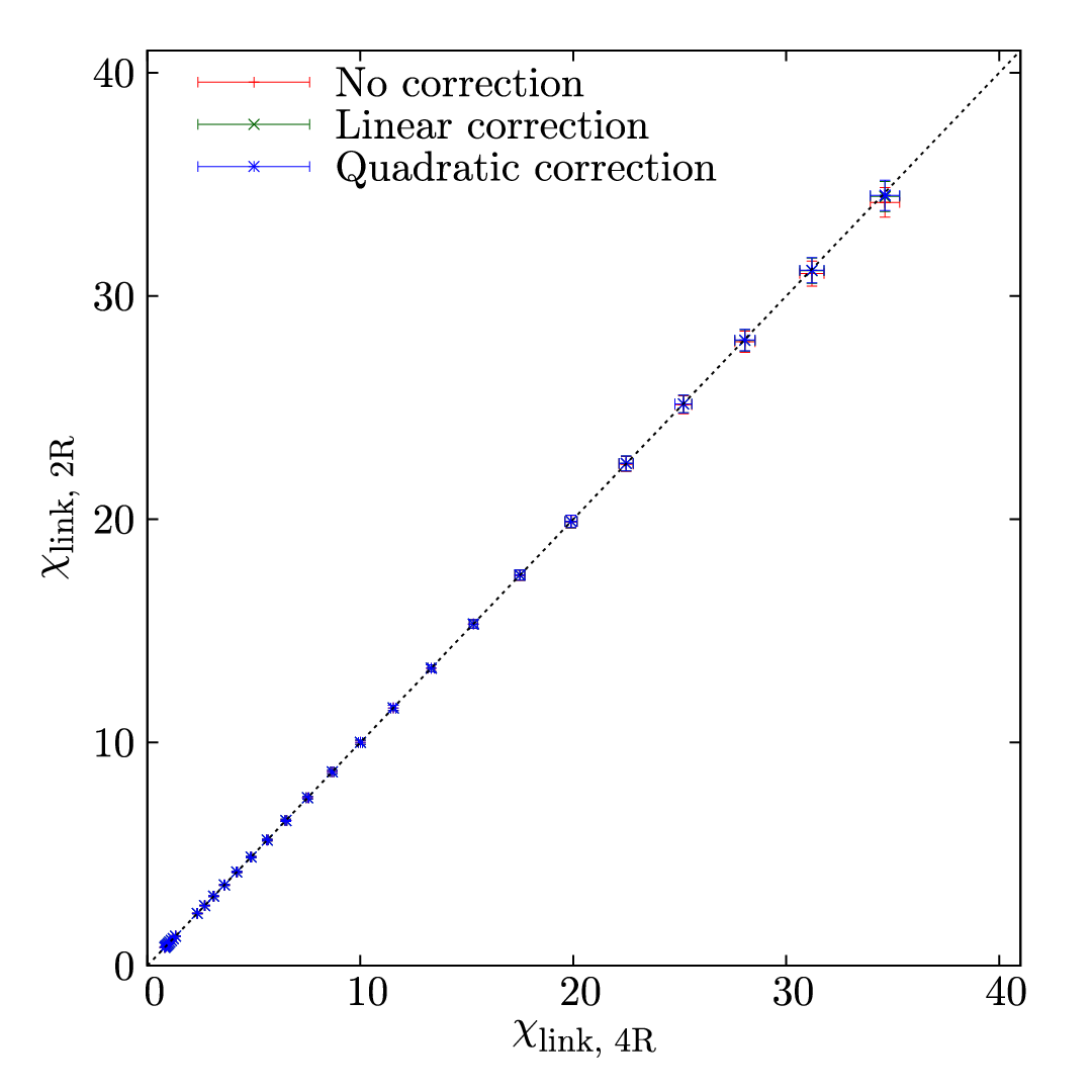
A very different test on the statistical quality of our data is the comparison of the values of $\chi_{\mathrm{link}}$ obtained using the different possible estimators for $\langle Q_{\mathrm{link}}\rangle^{2}$. We have an unbiased estimator if we use $Q_{\mathrm{link,4R}}^{(2)}$, see eq. (76), the linearly bias-corrected estimator $Q_{\mathrm{link,linear}}^{(2)}$ in eq. (74), and the quadratically bias-corrected estimator $Q_{\mathrm{link,quadratic}}^{(2)}$ in eq. (75). The different determinations are equal only if the total simulation time (in each sample) is much longer than the integrated autocorrelation time for $Q_{\mathrm{link}}$. As we see in figure 7–left, only computing $\chi_{\mathrm{link}}$ from the biased estimator $[Q_{\mathrm{link}}]_{2/2}^{2}$ results in a measurable bias. Once bias correction is taken into account, differences are only a fraction of the statistical error for each estimator. Nevertheless, the different statistical estimators are dramatically correlated. Hence, their difference might be significant. In figure 7–right we plot these differences for $L=24$ and $L=32$ as a function of temperature, in units of the statistical error for that difference. As we see, at the lowest temperatures for $L=32$, the bias for the estimate of $\chi_{\mathrm{link}}$ obtained from $Q_{\mathrm{link,linear}}^{(2)}$ is still measurable. Only the estimate from $Q_{\mathrm{link,quadratic}}^{(2)}$ is statistically compatible with the unbiased estimator. Since our data fully complies with our expectations, we consider the above analysis as a confirmation of our expectation $N\gg\tau_{\mathrm{int,Q_{\mathrm{link}}}},\tau_{\mathrm{exp}}\,.$

We carefully avoided to make decisions during thermalisation based on the values of physical quantities. However, one could worry about the possibility of important statistical correlations between the temperature random walk and interesting quantities. Such correlation could originate some small biases that would be difficult to eliminate. Fortunately, we have not found any correlation of this type. In figure 8 we show the correlation between $\tau_{\mathrm{exp}}$ and two important quantities: probability of the overlap being small and the energy.

We have plotted in figure 10—left the probability density at $q=0$ as a function of $T$ for all our lattices. There clearly is an enveloping curve in the region $T<T_{\mathrm{c}}$ with a decreasing, but positive, value of $P(0)$. In a mean-field setting [8] we expect this probability density to go to zero linearly in $T$. In order to check this, we have plotted $P(0)/T$ against $T$ in figure 10—right. As we can see, this expectation is fulfilled. For a similar study see [63]. We remark that the seemingly out of control value of $P(0)$ for our lowest temperature in $L=8$ is an artifact of the binary nature of the couplings (a finite system always has a finite energy gap). Indeed, in [64], the finite size behaviour of $P(0)$ for the Edwards-Anderson model with binary couplings was studied as a function of temperature. Finite-size effects on $P(0)$ turned out to be stronger close to $T=0$ than at finite temperature.

From a droplet model point of view, Moore et al. [21] have argued that the apparent lack of a vanishing limit for $P(0)$ in numerical work in the 1990s was an artifact of critical fluctuations. In fact, at $T_{\mathrm{c}}$, $P(0)$ diverges as $L^{\beta/\nu}$ while droplet theory predicts that, for very large lattices, it vanishes as $L^{-\zeta}$, with $\zeta\sim 0.2$, for all $T<T_{\mathrm{c}}$. These authors rationalise the numerical findings as a crossover between these two limiting behaviours. However, a numerical study at very low temperatures (so the critical regime is avoided) found for moderate system sizes a non-vanishing $P(0)$ [63]. Furthermore, we compute in section 4.3 a characteristic length for finite-size effects in the spin-glass phase, which turns out to be small at $T=0.703$.

We have plotted the Binder cumulant (6) for $T=0.625,0.703$ as a function of the system size in figure 11. As discussed in section 2.2, the evolution (and thermodynamical limit) of this observable is different in the droplet and RSB pictures:

where $1/\hat{\nu}=0.39(5)$ [26]. Since it is compatible with our best estimate for the replicon exponent, $\theta(0)=0.38(2)$, we prefer to use the second, more accurate value (there is some analytical ground for this identification [26]). We will attempt to distinguish between these two behaviours by fitting our data to (43) and (44).

These two-parameter fits are plotted in figure 11 and the resulting parameters are gathered in table 2. In the case of the RSB fit, Eq (44), we have included two error bars: the number enclosed in parentheses $(\,\cdot\,)$ comes from the statistical error in a fit fixing $1/\hat{\nu}$ to $\theta(0)$ and the one inside square brackets $[\,\cdot\,]$ is the systematic error due to the uncertainty in $\theta(0)$.

As it turns out, both fits have acceptable values of $\chi^{2}$ per degree of freedom (d.o.f.). However, the evolution of $B$ with $L$ is very slow, so in order to accommodate the limit value of $B(L\to\infty)=1$ consistent with the droplet picture, we have needed a very small exponent ($\zeta\sim 0.12$, smaller than the droplet prediction of $\zeta\approx 0.2$ [11]). On the other hand, according to droplet theory [11], the connected spatial correlation function at $q\!=\!q_{\mathrm{EA}}$ decays as $1/r^{\zeta}$. A direct study [26], however, indicates that these correlations decay as $1/r^{0.6}$.

The reader may find it disputable, from an RSB point of view, that a single power law should govern finite size effects. It would be rather more natural that corrections were of order

It turns out, however, that $\theta(q)$ hardly depends on $q$ (except on the neighbourhood of $q_{\mathrm{EA}}$), see [26] and Sect. 5. The neighbourhood of $q_{\mathrm{EA}}$ would produce a subleading correction of order $1/L^{0.6}$.

In any case, see section 6, we remark that the relevant regime for comparison with experimental work is $L\approx 110$, where both the RSB and the droplet fits predict that $B(T,L)$ is well above $1$ (see figure 11).

One of the features of the $P(q)$ about which droplet and RSB agree is the fate of its two symmetric peaks as we approach the thermodynamical limit. These should grow increasingly narrow and shift their position until they eventually become two Dirac deltas at $q=\pm q_{\mathrm{EA}}$. The actual value of $q_{\mathrm{EA}}$ is notoriously difficult to compute [25, 65, 66], see, however, [26].

Characterising the evolution of these peaks as we increase the system size is the goal of this section. We start by defining $q_{\mathrm{EA}}(L)$ as the position of the maximum of $P(q;L)$ (since the pdf is symmetric, we shall consider all overlaps to be positive in the remainder of this section). Thanks to the Gaussian smoothing procedure described in eq. (8), this maximum is very well defined. We compute its position by fitting the peak to a third-order polynomial (notice that the peaks are very asymmetric).

In order to further describe the peaks, we will also employ the half-widths $\sigma^{(\pm)}$ at half height $\bigl[P(q^{(\pm)})=P(q_{\mathrm{EA}}(L))/2\bigr]$:

where $q^{(-)}<q_{\mathrm{EA}}(L)<q^{(+)}$.

We have plotted these parameters as a function of temperature in figure 12. On table 3 we can see that the width of the peaks does decrease with a power law in $L$, although very slowly. The product $\sigma P(q_{\mathrm{EA}}(L))$ has a small dependence on $L$.

We can now extrapolate $q_{\mathrm{EA}}(L)$ to find the order parameter in the thermodynamical limit. A finite-size scaling study [26] shows that

where $1/\hat{\nu}=0.39(5)$. Yet, as discussed after eq. (44), we prefer to identify $1/\hat{\nu}$ with the replicon exponent, $\theta(0)=0.38(2)$. A disagreeing reader merely needs to double the error estimate in the extrapolation of $q_{\mathrm{EA}}$. Note that one should not attempt a three-parameter fit to eq. (47), as there are too few degrees of freedom. An independent estimate of $1/\hat{\nu}$ is required. Similar extrapolations were attempted in [47], with smaller system sizes ($L\leq 16$) and a lesser control over $1/\hat{\nu}$.

References

- [1] Mydosh J A 1993 Spin Glasses: an Experimental Introduction (London: Taylor and Francis)
- [2] Fisher K H and Hertz J A 1993 Spin Glasses (Cambridge University Press)
- [3] Ballesteros H G, Cruz A, Fernandez L A, Martin-Mayor V, Pech J, Ruiz-Lorenzo J J, Tarancon A, Tellez P, Ullod C L and Ungil C 2000 Phys. Rev. B 62 14237
- [4] Palassini M and Caracciolo S 1999 Phys. Rev. Lett. 82 5128
- [5] Gunnarsson K, Svendlindh P, Nordblad P, Lundgren L, Aruga H and Ito A 1991 Phys. Rev. B 43 8199
- [6] Franz S, Mézard M, Parisi G and Peliti L 1998 Phys. Rev. Lett. 81 1758
- [7] Franz S, Mézard M, Parisi G and Peliti L 1999 J. Stat. Phys. 97 459
- [8] Mézard M, Parisi G and Virasoro M 1987 Spin-Glass Theory and Beyond (Singapore: World Scientific)
- [9] Marinari E, Parisi G, Ricci-Tersenghi F, Ruiz-Lorenzo J J and Zuliani F 2000 J. Stat. Phys. 98 973
- [10] McMillan W L 1984 J. Phys. C 17 3179
- [11] Bray A J and Moore M A 1987 Heidelberg Colloquium on Glassy Dynamics (Lecture Notes in Physics no 275) ed van Hemmen J L and Morgenstern I (Berlin: Springer)
- [12] Fisher D S and Huse D A 1986 Phys. Rev. Lett. 56 1601
- [13] Fisher D S and Huse D A 1988 Phys. Rev. B 38 37
- [14] Gardner E 1984 J. Phys. (France) 45 1755
- [15] Krzakala F and Martin O C 2000 Phys. Rev. Lett. 85 3013
- [16] Palassini M and Young A P 2000 Phys. Rev. Lett. 85 3017
- [17] Contucci P, Giardinà C, Giberti C and Vernia C 2006 Phys. Rev. Lett. 96 217204
- [18] Contucci P, Giardinà C, Giberti C, Parisi G and Vernia C 2007 Phys. Rev. Lett 99 057206
- [19] Contucci P, Giardinà C, Giberti C, Parisi G and Vernia C 2009 Phys. Rev. Lett 103 017201
- [20] Jörg T and Katzgraber H G 2008 Phys. Rev. Lett. 101 197205
- [21] Moore M, Bokil H and Drossel B 1998 Phys. Rev. Lett. 81 4252
- [22] Belletti F, Mantovani F, Poli G, Schifano S F, Tripiccione R, Campos I, Cruz A, Navarro D, Perez-Gaviro S, Sciretti D, Tarancon A, Velascco J L, Tellez P, Fernandez L A, Martin-Mayor V, Muñoz Sudupe A, Jimenez S, Maiorano A, Marinari E and Ruiz-Lorenzo J J (Janus Collaboration) 2006 Computing in Science and Engineering 8 41
- [23] Belletti F, Cotallo M, Cruz A, Fernandez L A, Gordillo A, Maiorano A, Mantovani F, Marinari E, Martin-Mayor V, Monforte J, Muñoz Sudupe A, Navarro D, Perez-Gaviro S, Ruiz-Lorenzo J J, Schifano S F, Sciretti D, Tarancon A, Tripiccione R and Velasco J (Janus Collaboration) 2008 Comp. Phys. Comm. 178 208
- [24] Belletti F, Cotallo M, Cruz A, Fernandez L A, Gordillo-Guerrero A, Guidetti M, Maiorano A, Mantovani F, Marinari E, Martin-Mayor V, Muñoz Sudupe A, Navarro D, Parisi G, Perez-Gaviro S, Ruiz-Lorenzo J J, Schifano S F, Sciretti D, Tarancon A, Tripiccione R, Velasco J and Yllanes D (Janus Collaboration) 2008 Phys. Rev. Lett. 101 157201
- [25] Belletti F, Cruz A, Fernandez L A, Gordillo-Guerrero A, Guidetti M, Maiorano A, Mantovani F, Marinari E, Martin-Mayor V, Monforte J, Muñoz Sudupe A, Navarro D, Parisi G, Perez-Gaviro S, Ruiz-Lorenzo J J, Schifano S F, Sciretti D, Tarancon A, Tripiccione R and Yllanes D (Janus Collaboration) 2009 J. Stat. Phys. 135 1121
- [26] Álvarez Baños R, Cruz A, Fernandez L A, Gil-Narvion J M, Gordillo-Guerrero A, Guidetti M, Maiorano A, Mantovani F, Marinari E, Martin-Mayor V, Monforte-Garcia J, Muñoz Sudupe A, Navarro D, Parisi G, Perez-Gaviro S, Ruiz-Lorenzo J, Schifano S F, Seoane B, Tarancon A, Tripiccione R and Yllanes D (Janus Collaboration) 2010 (Preprint arXiv:1003:2943)
- [27] Fernandez L A, Martin-Mayor V, Perez-Gaviro S, Tarancon A and Young A P 2009 Phys. Rev. B 80 024422
- [28] Edwards S F and Anderson P W 1975 J. Phys. F 5 975
- [29] Edwards S F and Anderson P W 1976 J. Phys. F 6 1927
- [30] Toulousse G 1977 Communications on Physics 2 115
- [31] Hasenbusch M, Pelissetto A and Vicari E 2008 J. Stat. Mech L02001
- [32] Hasenbusch M, Pelissetto A and Vicari E 2008 Phys. Rev. B 78 214205
- [33] Marinari E, Parisi G, Ricci-Tersenghi F and Ruiz-Lorenzo J J 1998 Journal of Physics A: Math. and Gen. 31 L481
- [34] Fernandez L A, Martin-Mayor V and Yllanes D 2009 Nucl. Phys. B 807 424–454
- [35] de Dominicis C, Kondor I and Temesvári T 1998 Spin glasses and random fields ed Young A P (Singapore: World Scientific)
- [36] de Dominicis C, Kondor I and Temesvári T 1999 Eur. Phys. J. B 11 629
- [37] de Dominicis C and Giardina I 2006 Random Fields and Spin Glasses (Cambridge, England: Cambridge University Press)
- [38] Martin-Mayor V 2007 Phys. Rev. Lett. 98 137207
- [39] Macdowell L G, Shen V and Errington J R 2006 J. Chem. Phys. 125120 034705
- [40] Marinari E, Parisi G, Ruiz-Lorenzo J J and Zuliani F 1999 Phys. Rev. Lett. 82 5176
- [41] Contucci P and Giardinà C 2005 Phys. Rev. B 72 014456
- [42] Contucci P 2003 J. Phys. A: Math. Gen. 36 10961
- [43] Contucci P and Giardinà C 2005 Ann. Henri Poincare 6 915
- [44] Contucci P and Giardinà C 2007 J. Stat. Phys. 126 917
- [45] Parisi G 1998 (Preprint cond-mat/9801081)
- [46] Parisi G and Ricci-Tersenghi F 2000 J. Phys. A: Math. Gen. 33 113
- [47] Iñiguez D, Parisi G and Ruiz-Lorenzo J J 1996 J. Phys. A: Math. and Gen. 29 4337
- [48] Fernandez L A, Martin-Mayor V, Parisi G and Seoane B 2010 Phys. Rev. B 81 134403
- [49] Jimenez S, Martin-Mayor V, Parisi G and Tarancon A 2003 J. Phys. A: Math. and Gen. 36 10755
- [50] Franz S, Parisi G and Virasoro M 1992 J. Phys. (France) 2 1869
- [51] Amit D J and Martin-Mayor V 2005 Field Theory, the Renormalization Group and Critical Phenomena 3rd ed (Singapore: World Scientific)
- [52] Chayes J, Chayes L, Fisher D S and Spencer T 1986 Phys. Rev. Lett. 57 2999
- [53] Maiorano A, Martin-Mayor V, Ruiz-Lorenzo J J and Tarancón A 2007 Phys. Rev. B 76 064435
- [54] Belletti F, Guidetti M, Maiorano A, Mantovani F Schifano S F, Tripiccione R, Cotallo M, Perez-Gaviro S, Sciretti D, Velasco J L, Cruz A, Navarro D, Tarancon A, Fernandez L A, Martin-Mayor V, Muñoz-Sudupe A, Yllanes D, Gordillo-Guerrero A, Ruiz-Lorenzo J J, Marinari E, Parisi G, Rossi M and Zanier G (Janus Collaboration) 2009 Computing in Science and Engineering 11 48
- [55] Hukushima K and Nemoto K 1996 J. Phys. Soc. Japan 65 1604
- [56] Marinari E 1998 Advances in Computer Simulation ed Kerstész J and Kondor I (Springer-Berlag)
- [57] Ogielski A 1985 Phys. Rev. B 32 7384
- [58] Bittner E, Nußbaumer A and Janke W 2008 Phys. Rev. Lett. 101 130603
- [59] Sokal A D 1997 Functional Integration: Basics and Applications (1996 Cargèse School) ed DeWitt-Morette C, Cartier P and Folacci A (New York: Plenum)
- [60] Frigo M and Johnson S G 2005 Proceedings of the IEEE 93 216
- [61] Ballesteros H G, Fernandez L A, Martin-Mayor V and Muñoz Sudupe A 1997 Nucl. Phys. B 483 707
- [62] Janus Collaboration (in preparation)
- [63] Katzgraber H, Palassini M and Young A 2001 Phys. Rev. B 63 184422
- [64] Palassini M and Young A P 2001 Phys. Rev. B 63 140408(R)
- [65] Perez-Gaviro S, Ruiz-Lorenzo J J and Tarancón A 2006 J. Phys. A: Math. Gen. 39 8567–8577
- [66] Iñiguez D, Marinari E, Parisi G and Ruiz-Lorenzo J J 1997 J. Phys. A: Math. and Gen. 30 7337
- [67] Josephson B D 1966 Phys. Lett. 21 608
- [68] Luescher M, Weisz P and Wolff U 1991 Nucl. Phys. B 359 221
- [69] Kim J K 1993 Phys. Rev. Lett. 70 1735
- [70] Caracciolo S, Edwards R G, Ferreira S J, Pelissetto A and Sokal A D 1995 Phys. Rev. Lett 74 2969
- [71] Caracciolo S, Edwards R G, Pelissetto A and Sokal A D 1995 Phys. Rev. Lett 75 1891
- [72] Jörg T 2006 Phys. Rev. B 73 224431
- [73] Moore M 2010, (Preprint arXiv:1005.0561).
- [74] Bouchaud J P, Dupuis V, Hammann J and Vincent E 2001 Phys. Rev. B 65 024439
- [75] Katzgraber H and Young A 2003 Phys. Rev. B 67 134410
- [76] Detrey J and de Dinechin F 2007 Microprocessors and Microsystems 31 537
- [77] Press W H, Teukolsky S A, Vetterling W T and Flannery B P 1992 Numerical Recipes in C 2nd ed (Cambridge: Cambridge University Press)