Geometrical origin of chaoticity in the bouncing ball billiard
L. Mátyás1, and I. F. Barna2
1 Sapientia University, Department of Technical and Natural Sciences,
Libertătii sq. 1,
530104 Miercurea Ciuc, Romania.
2 KFKI Atomic Energy Research Institute of the Hungarian Academy of
Sciences, (AEKI) P.O. Box 49, 1525 Budapest, Hungary.
Abstract
We present a study of the chaotic behavior of the bouncing ball billiard. The work is realised on the purpose of finding at least certain causes of separation of the neighbouring trajectories. Having in view the geometrical construction of the system, we report a clear origin of chaoticity of the bouncing ball billiard. By this we claim that in case when the floor is made of arc of circles - in a certain interval of frequencies - a lower bound for the maximal Ljapunov can be evaluated by semianalical techniques.
1 Introduction
Deterministic features of transport has been studied in different problems [1]. These works has also shown that transport may be related to the chaotic aspects of the dynamics [2].
The idea of bouncing ball was studied in different problems where analytical approximations [3] and comprehensive numerical works can also be found [4]. The analytical approximations have been shown the possible evidence of bifurcations while the numerical works presented chaotic regimes of the bouncing ball system.
The bouncing ball billiard as a spatial extension of the one dimensional bouncing ball problem has been introduced in [5]. This first work enhances the irregular diffusivity of the system which is similar to certain models of transport [6]. The following work has outlined the spiral modes in the phase space of this problem [7] and also pointed out its relevance on granular matter [8]. Idealised versions where the bounces are performed without loss of energy, i.e. the restitution coefficient is one, and there is no oscillation of the floor may be found in [9].
The chaoticity of the sawtooth type of the bouncing ball billiard has been studied in [10], with considerable theoretical background [11]. Considering the problem as a gravitational billiard, aspects on chaotic features are also approached by numerical methods in [12].
The present work focuses on the geometrical origin of chaoticity of the bouncing ball billiard where it is investigated the impact of the curvature of the arcs of circles on the maximal Ljapunov exponent. The derivation shows, that in case of resonance one may give semianalitical estimates on chaotic behavior.
The study on manifolds for multi-dimensional billiards related to geometric properties is presented in [13].
From the practical point of view the reaction of with on surface, which is under thermal excitation, the molecules performs diffusive motion on the surface before the reaction would occur [14].
Quasi-deterministic aspects on diffusion may occur in the behaviour of of certain species where in the process of food searching one can find a randomness, but there is also a kind of determinism because the animals may have certain remembrances on the places where they found food in the past [15].
The article is organised as follows. In Section 2 we shortly describe the bouncing ball billiard system. The Section 3 makes a presentation of that frequency region where the semianalical approaches to some extent are possible. Section 4 shows an evaluation which has a semi-empirical and analytical background giving a lower bound for the maximal Ljapunov exponent. Finally, Section 5 discusses the similarities and differences of the analytical and real value of the maximal Ljapunov exponent.
2 The bouncing ball billiard
At this point we make a review of the most important features of the bouncing ball problem. The system studied is a point particle, which bounces on a floor realised of arc of circles [16]. The floor is oscillating with a frequency corresponding to a circular frequency . The system is presented below.

The bouncing ball billiard from the point of view of the diffusion was presented in a comprehensive way in [5, 7]. The main conclusions are that the system possesses irregular diffusion, and the principal maximas for the diffusion occurs at the resonances. These resonances are at the frequencies, where the time of the flight becomes equal or multiple of the period of vibration applied.
The bouncing ball billiard that we study in this paper, with the floor formed by circular scatterers, is depicted in Fig. 1.
The equations of motion of this system are presented as follows: The particle performs a free flight between two collisions in the gravitational field . Consequently, its coordinates and velocities at time immediately before the collision and its coordinates and velocities at time immediately after the collision are related by the following equations
| (1) | |||||
| (2) | |||||
| (3) | |||||
| (4) |
At the collisions the change of the velocities is given by
| (5) | |||||
| (6) |
where is the velocity of the corrugated floor. We distinguish between the two different velocity components relative to the normal vector at the surface of the scatterers, where the scatterers are represented by the arcs of the circles forming the floor. , and , is the normal and tangential components of the particle’s, respectively the floor’s velocity with respect to the surface at the scattering point. Correspondingly, we introduce two different restitution coefficients and that are perpendicular, respectively tangential to the normal.
As in case of the vertically bouncing ball problem we assume that the floor oscillates sinusoidally, , where and are the amplitude respectively the frequency of the vibration, see Fig.1.
The radius of circles are =15mm and the restitution coefficients , respective . It is important that the slope on the arcs of the circles is very shallow. The distance between two arc of circles is . By this terms proportional with or less are considered terms with second - or higher - order.
2.1 Considerations on the chaoticity of the bouncing ball
The chaos of the bouncing ball which spatially is a one dimensional system and which is performed on the vertical direction has been discussed in [4].
If we consider the initial displacement and the displacement after bounces between neighboring trajectories for the one dimensional vertically bouncing ball, then the Ljapunov exponent may be evaluated: . The main problem is that at certain frequencies the ball may be stucked on the surface. Because the neigbouring trajectory usually is also stucked, i.e. becomes zero, consequently in such cases the Ljapunov exponent is simply undefined.
Of coarse one may discuss on chaotic regimes between two stucks, but this is the reason why in general considerations about the chaoticity of the vertically bouncing ball should be done in a very careful way.
In spite of the fact that in two dimensions it is almost impossible to have neighboring orbits stucked at the same place, the following study will try to avoid that frequency regions where stucking orbits might be possible.
3 General considerations
We discuss the chaoticity of the bouncing ball billiard at the frequency region where the 1/1 resonance holds. The approximation we try to make is semi-empirical and the considerations are presented below. The first observation we make is, that the time of the flight between subsequent collision at 1/1 resonance is approximately the same. We note this time with and corresponds to that time while the particle makes one bounce and it is close to the time while the floor makes one complete oscillation. Subsequent values of at 1/1 resonance are shown below
| time of flight | collision no |
|---|---|
| 0.0183 | 29 |
| 0.0191 | 30 |
| 0.0185 | 31 |
| 0.0190 | 32 |
| 0.0184 | 33 |
One can see that these values do not differ too much. They cannot be the same, for instance because the surface is not flat, but they are close to each other and around a specific value.
The other observation is, that the first resonance manifests so that the elongation almost reaches its maximum , and the particle meets the floor for almost all cases very close to this height - see fig. 2.
4 Geometrical origin of chaoticity
We consider one component of the velocity, namely the horizontal one . We are interested in change in difference of the horizontal component of the velocities of two neighboring trajectories. By this we try to make an estimate of a lower bound of the Ljapunov exponent, which manifests on the direction of the phase space, which would also give a picture on the horizontal chaoticity of this problem.
The figure below fig. 2 shows two trajectories, starting from the same place, with slightly different velocity vectors. The picture is at 1/1 resonance, where after a certain transient the bounces are made a little bit above the vertical coordinate mm which denotes the amplitude.

We assume that at the starting point there is a difference in angles but not in the magnitude of the velocities . This initial deflection in angles we denote by . The corresponding difference in initial velocities we denote by . Because of this initial deflection in angle there will be at final arrival a change in horizontal coordinates .
Due to the convex curvature of the arcs characterized by the radius , the displacement at the arrival on this curvature will cause further deflection in angles after one collision which we denote by . This cause a final difference in the horizontal component of velocities after the first bounce .
The rate of exponential separation of the trajectories after such a bounce due to the finite radius we denote with
| (7) |
At the launch of the trajectory we consider the magnitude of the velocity , the angles relative to the vertical are and , the complementer angles are and where as it was mentioned above
| (8) |
where the higher order terms means terms which are proportional with at least the second power of . Correspondingly if is the angle between the directions of trajectories after the first bounce
| (9) |
Because there is a free flight in gravitational field and the arcs are with shallow slope practically , very precisely their difference is a second order term. We mention, that is also small as one can see on the fig. 2, so its product with is also considered a value with second order. 11 1 Even if a term proportional with or would be kept, at the end where the average value is calculated for or it drops out or it is proved to be of higher order.
As a result we get for the value , which has a definite contribution due to the finite value of
| (10) |
where one can see that the ratio between the deflection of the angles after the bounce and before the bounce counts.
The bounce is presented on Fig. 3.

Based on Fig. 3 we can conclude that the deflection between the two reflected trajectories () one hand is due to the initial deflection . For the reflected trajectories there is a contribution due to the curvature. If the point of incidence of the first trajectory is at then the point of incidence of the second one is at . The incident angles relative to the normal differs by and in addition the reflected angles - on the Fig. 3 - and has also a difference . Consequently the term has to be counted twice.
| (11) |
Inserting this relation in eq.(10) one gets
| (12) |
At the arriving point on the surface the initial difference will cause a displacement . This means that on the arc of the circle the trajectories will arrive at a difference as one can see on fig. 3. Now follows the evaluation of and correspondingly of the .
The length is due to the difference in angles of the velocities, at the starting point. The first one is launched at an angle the other one with an angle . At the end one of the particles arrives at , the other one at
| (13) |
where is the angle of the velocity made with the horizontal direction of the first trajectory at the starting point. During the evaluation we make the approximation, that is approximately and or the differences are at least second order in , and are included in the higher order terms.
| (14) |
At this point one can see that - here being the incident angle relative to the vertical - can be neglected, consequently yields the following value
| (15) |
If we take into account that the time for the flight is then
| (16) |
By this we get for the value in leading order
| (17) |
where the logarithm has been expanded, and terms proportional with have been also considered as being of higher order.
The average of means averaging the expression above. By this the higher order terms vanishes or becomes smaller so they remain of higher order. Consequently it reduces to the average of the time of the flight . Its average is given by the period of oscillations resulting for in leading order
| (18) |
Because is a manifestation of the separation of the neighboring trajectories in the direction due to the geometry, consequently this value can be considered a lower bound for the maximal Ljapunov exponent.
4.1 The case of two periodic orbits
As it is pointed out in the work [3] - with increasing the frequency - bifurcation of the resonant trajectory may be possible. This means that the time of flight consists of a shorter and a longer time alternating one after the other which we denote by and , but they still do not differ too much from each other. 22 2 In general in the case of the bouncing ball billiard to have a considerable difference between and even it is not possible, or because the dynamics enters in further bifurcations, or simply it crashes to a scenario with lots of sticking orbits.
In such case the approximation that have been presented previously are still valid and one gets after two consequent flights - one is shorter, one is longer -
| (19) |
The argument of the logarithm can be written as
| (20) |
After the expansion to the first order we have
| (21) |
In the numerator of the second fraction the decompositions are made
| (22) |
Finally we arrive to the relation
| (23) |
This expression can be averaged and the term proportional with is still too small and is considered of second order. The average of the last expression yields the value
| (24) |
where and represents the average values of the respective . Because even in the case of the two periodic orbit equals an average time flight which is the inverse of that frequency where the dynamics is already bifurcated. This is in fact an interval of frequencies, so the latter formula for two periodic orbits still shows a strong analogy with eq. (18) and it may be written
| (25) |
This latter formula shows that the relation (18) may be valid for the full 1/1 resonance and for bifurcated trajectories not too far from it.
5 The real value of the maximal Ljapunov exponent
In this section we discusses connections of the geometry with the chaoticity. The relation (18) in case of the 1/1 resonance at a given gravitational field has a characteristic time of flight . Because of this reason, one may consider that one of the most relevant dependence of the maximal Ljapunov exponent from practical purposes is in terms of the radius. So in this section we restrict ourselves to the case of the frequency Hz when the first resonance is fully developed. 33 3 The interval where we expect a validity of the relation (18) is a frequency region Hz. The validity sometimes may be even wider, however there is a slight dependence of the endpoints of the interval on , consequently it has been chosen a common domain in which the resonance or eventually the bifurcated scenario holds for different radii we discuss below. The following figure illustrates the numerical values of the maximal Ljapunov exponent in terms of inverse of the radius. Consequently we start at a curvature 1/24 mm-1 and we end at a curvature 1/16 mm-1. The endpoints are also motivated by the works [5, 7].
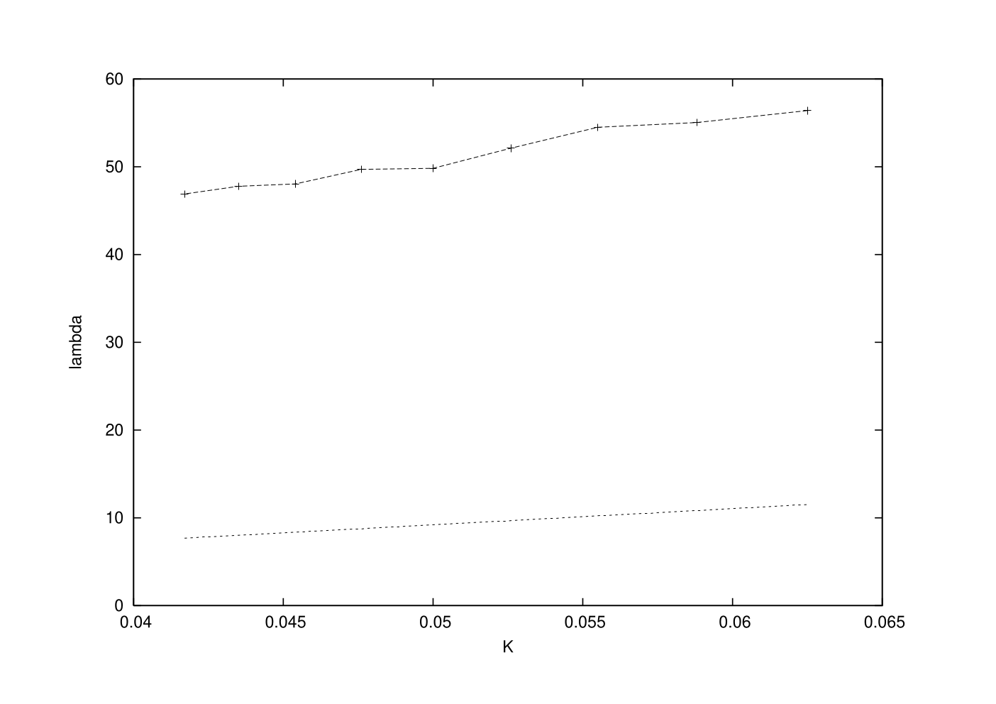
As one can see the maximal Ljapunov exponent increases as the curvature - the inverse of the radius - increases. This is normal because a smaller radius implies a stronger separation of neighboring trajectories. From quantitative point of view both the numerical and the analytical evaluations has similar behavior - as it is shown on the fig. 4.
Regarding the quantitative aspects the evaluation (18) is considerably below of the real value. Partly because the analytical evaluation is just a projection. On the other hand the evaluation wants to detect only the geometrical effects on the chaoticity. Of coarse considerable other effects may have an important role on the chaoticity, but the study of such aspects will need further work.
We thank Rainer Klages for comments and encouragement.
References
- [1] P. Gaspard, Chaos, Schattering and Statistical Mechanics, Cambridge University Press, Cambridge, England, (1998); J.R.Dorfman, An Introduction to Chaos on Nonequilibrium Statistical Mechanics, Cambridge University Press, Cambridge (1999).
- [2] R. Klages, J.R. Dorfman, Phys. Rev. Lett. 74, 387 (1995); L. Mátyás, T. Tél and J. Vollmer, Phys. Rev. E 69, 016205 (2004); S. Viscardy, P. Gaspard, Phys. Rev. E 68 041205 (2003).
- [3] J. Guckenheimer, P.J. Holmes, Nonlinear Oscillations, Dynamical Systems and Bifurcations of the Vector Fields, 5th ed., Springer, New York, 1997.
- [4] A. Mehta, E.M. Luck, Phys. Rev. Lett. 65 393 (1990), E.M. Luck and A. Mehta, Phys. Rev. E 48, 3988 (1993).
- [5] L. Matyas, R. Klages, Physica D 187 165 (2004).
- [6] N. Korabel and R. Klages, Phys. Rev. Lett. 89, 214102 (2002); N. Korabel, A.V. Chehkin, R. Klages, I.M. Sokolov and V.Yu. Gonchar Europhys. Lett. 70, 63 (2005).
- [7] R. Klages, I.F. Barna, L. Matyas, Physics Letters A 333 79 (2004).
- [8] W. Losert, D. Cooper, J. Gollub, Phys. Rev. E 48 3988 (1993); Z. Farkas, F. Szalai, D. Wolf, T. Vicsek, Phys. Rev. E 65 022301 (2002); A. Prevost, D. Egolf, J. Urbach, Phys. Rev. Lett. 89 084031 (2002).
- [9] T. Harayama, P. Gaspard, Phys. Rev. E 64 036215 (2001).
- [10] A. de Wijn and H. Kantz, Phys. Rev. E 75 046214 (2007).
- [11] A. Riegert, N. Baba, K. Gelfert, W. Just and H. Kantz, Phys. Rev. Lett. 94, 054103 (2005).
- [12] A.Z. Gorski, T. Srokowski, Acta Physica Polonica B, 37 2561 (2006).
- [13] T. Balint, N. Chernov D. Szász, I.P. Tóth, Geometry of multi-dimensional dispersing Billiards
- [14] A von Oertzen, H. H. Rotermund and S. Nettesheim, Chem. Phys. Lett. 199, 131 (1992).
- [15] T. Hartel, Sz. Nemes, Gy. Mara, Acta Zoologica Lituanica 17, 56 (2007).
- [16] One can also study the bounce of a particle with finite radius, that can be reduced to a point particle problem [5]