Regenerating hyperbolic cone 3-manifolds from dimension 2

Joan Porti Note: Partially supported by the Spanish Micinn through grant MTM2009-07594 and prize ICREA ACADEMIA 2008

August 24, 2026

Abstract

We prove that a closed 3-orbifold that fibers over a hyperbolic polygonal 2-orbifold admits a family of hyperbolic cone structures that are viewed as regeneration of the polygon, provided that the perimeter is minimal.

1 Introduction

The space of hyperbolic cone 3-manifolds with fixed topological type and with cone angles less than $\pi$ is well understood by [33], but the boundary of this space is not. The aim of this paper is to establish a regeneration result in the spirit of Hodgson [22], that goes from a hyperbolic 2-orbifold, viewed as a collapsed 3-orbifold, to a family of hyperbolic cone 3-manifolds with decreasing cone angles, starting at $\pi$ . The 3-orbifold is Seifert fibered, and those cone manifolds appear in the proof of the orbifold theorem; however, none of the approaches shows the explicit collapse, as the Seifert fibration is constructed by other methods [9, 6, 4, 3].

Let $\mathcal{O}^{3}$ be a closed and orientable 3-orbifold, which is Seifert fibered over a two orbifold $P^{2}$ :

S^{1}\to\mathcal{O}^{3}\to P^{2}.

The branching locus of $\mathcal{O}^{3}$ is a link or a trivalent graph $\Sigma_{\mathcal{O}^{3}}$ . Its edges and circles are grouped in two, horizontal (if they are transverse to the fibers) or vertical (if they are fibers):

\Sigma_{\mathcal{O}^{3}}=\Sigma_{\mathcal{O}^{3}}^{Hor}\cup\Sigma_{\mathcal{O}^{3}}^{Vert}.

Points in $\Sigma_{\mathcal{O}^{3}}^{Hor}$ project to the mirror and dihedral points of $P^{2}$ . Assume that the orbifold $P^{2}$ is a hyperbolic Coxeter group, generated by reflections on a hyperbolic polygon whose angles are $\pi$ over an integer. Thus $P^{2}$ is a polygon with mirror points at the edges, and dihedral points at the vertices. We may assume also that $P^{2}$ has possibly a single cone point in its interior. For instance, $S^{3}$ with branching locus a Montesinos link is an example of such fibration.

We view the Seifert fibration as a transversely hyperbolic foliation, hence with a developing map

D_{0}\!:\!\tilde{\mathcal{O}}^{3}\to\mathbf{H}^{2}

that factors through the universal covering of $P^{2}$ .

According to Kerckhoff’s proof of Nielsen conjecture [23], there is a unique point in the Teichmüller space that minimizes the perimeter of $P^{2}$ . Let

P^{2}_{min}

denote the orbifold equiped with this hyperbolic structure.

The main result of this paper is the following:

Theorem 1.1.

Assume that $P^{2}$ has at most one cone point in its interior. There exists a family of hyperbolic cone manifold structures $C(\alpha)$ on $|\mathcal{O}^{3}|$ , with singular locus $\Sigma_{\mathcal{O}^{3}}$ and cone angle $\alpha\in(\pi-\varepsilon,\pi)$ on $\Sigma_{\mathcal{O}^{3}}^{Hor}$ and constant angles (the orbifold ones) on $\Sigma_{\mathcal{O}^{3}}^{Vert}$ , so that

\lim_{\alpha\to\pi^{-}}C(\alpha)=P^{2}_{min}

for the Gromov-Hausdorff convergence. Moreover the developing maps converge to the developing map of the transversely hyperbolic foliation.

The orbifold $\mathcal{O}^{3}$ can be viewed as a cone manifold $C(\pi)$ with geometry $\widetilde{SL_{2}(\mathbf{R})}$ or $\mathbf{H}^{2}\times\mathbf{R}$ , depending on the Euler number. With one of these geometries, the singular edges and circles are either horizontal (with angle $\pi$ ) or vertical, as those geometries are fibered. The theorem generalizes to those cone manifolds, without assuming that the vertical angles are $2\pi/n$ , just that the basis is a polygon with angles $\leq\pi/2$ . This means that if $q\geq 1$ is the order of a singular fiber (with $q=1$ if the fiber is regular), and if $\vartheta_{i}\leq 2\pi$ is the cone angle, then we require $\vartheta_{i}/q\leq\pi$ .

Let $k$ be the number of circles and edges on $\Sigma_{C(\pi)}^{Hor}$ . Choose weights $w_{1},\ldots,w_{k}\in\mathbf{R}_{+}=\{x\in\mathbf{R}\mid x>0\}$ on these horizontal components. Those induce weights

\mathcal{W}=\{\overline{w}_{1},\ldots,\overline{w}_{n}\}

on the edges of $P^{2}$ , just by adding the two weights of the mirror points of the fiber of any interior point of the edge, ie. $\overline{w}_{i}=w_{j_{i}}+w_{k_{i}}$ . Of course if $k=1$ , then $\mathcal{W}$ is the constant weight. If $e_{1},\ldots,e_{n}$ are the edges of $P^{2}$ , with lengths $|e_{1}|,\ldots,|e_{n}|$ , the $\mathcal{W}$ -perimeter is defined as

\overline{w}_{1}|e_{1}|+\cdots+\overline{w}_{n}|e_{n}|.

We will show (Proposition 1.5) that in the set of hyperbolic structures on a polygon with ordered angles $\vartheta_{1}/2q_{1},\ldots,\vartheta_{n}/2q_{n}$ there is a unique minimizer of the $\mathcal{W}$ -perimeter, that we denote $P^{2}_{\mathcal{W}-min}.$

Theorem 1.2.

Let $C(\pi)$ be a closed, orientable cone manifold with geometry $\widetilde{SL_{2}(\mathbf{R})}$ or $\mathbf{H}^{2}\times\mathbf{R}$ with cone angles $\leq 2\pi$ , and with space of fibers a polygon $P^{2}$ with angles $\leq\pi/2$ . There exists a family of hyperbolic cone manifold structures $C(\alpha_{1},\ldots,\alpha_{k})$ with cone angles $\alpha_{i}=\pi-w_{i}t$ , for $i=1,\ldots,k$ and $t\in(0,\varepsilon)$ on $\Sigma_{\mathcal{O}^{3}}^{Hor}$ , and constant angles on $\Sigma_{\mathcal{O}^{3}}^{Vert}$ , such that

\lim_{t\to 0^{+}}C(\alpha_{1},\ldots,\alpha_{k})=P^{2}_{\mathcal{W}-min}

for the Gromov-Hausdorff converge.

A version of Theorem 1.1 was stated in Hodgson’s thesis [22]. In particular, Hodgson showed that the minimizer of the perimeter corresponds to a singularity in the variety of representations of $\mathcal{O}^{3}\smallsetminus\Sigma_{\mathcal{O}^{3}}$ . However, to construct the path of representations requires further detail, done here. For the construction of the developing maps we use an approach different from [22].

The idea of regenerating from Kerckhoff minimizers is also related to a theorem of Series on pleated surfaces [29], where as an application she also obtains a family of cone manifolds.

Theorem 1.1 needs to assume that there is at most one cone point in the interior of the polygon, otherwise $\mathcal{O}^{3}\setminus\Sigma_{\mathcal{O}^{3}}$ would contain an essential torus, contradicting the existence of hyperbolic cone structures.

Refer to caption — Figure 1: Example of fibered orbifold: $S^{3}$ with branching locus this link. The base is a quadrilateral.

We make the following assumption along the paper:

Remark 1.3.

We may assume that $P^{2}$ has no interior cone point: If the interior of $P^{2}$ has one cone point, then we consider the orbifold covering that unfolds this point and work equivariantly.

Concerning the equivariance, the structure of $P^{2}$ that minimizes the perimeter is unique, by Kerckhoff [23], hence equivariant. The structure of the hyperbolic cone manifolds is also equivariant because it is unique, by Weiss’ global rigidity [34]. Notice that two or more cone points would not produce a polygon when unfolding, but an orbifold with more complicated underlying space.

Let us show a consequence of Theorem 1.2 for hyperbolic polyhedra. Fix $n$ positive real numbers

0<\beta_{1},\ldots,\beta_{n}\leq\pi/2,

satisfying $\sum(\pi-\beta_{i})>\pi$ . By Andreev theorem, for any choice of $\alpha_{1},\ldots,\alpha_{n}$ , $\alpha_{1}^{\prime},\ldots,\alpha_{n}^{\prime}$ satisfying

0<\alpha_{i},\alpha_{i}^{\prime}<\pi/2,\qquad\alpha_{i}+\alpha_{i+1}>\pi-\beta_{i},\quad\textrm{ and }\quad\alpha_{i}^{\prime}+\alpha_{i+1}^{\prime}>\pi-\beta_{i},

there exists a unique hyperbolic polyhedron with the combinatorial type of a prism with an $n$ -edged polygonal base, with dihedral angles at the “vertical” edges $\beta_{1},\cdots,\beta_{n}$ , angles $\alpha_{1},\ldots,\alpha_{n}$ at the respective $n$ “horizontal” edges of the top face, and $\alpha_{1}^{\prime},\ldots,\alpha_{n}^{\prime}$ at the respective $n$ horizontal edges of the bottom face. They are arranged so that the edges with angles $\alpha_{i}$ , $\beta_{i}$ , $\alpha_{i}^{\prime}$ and $\beta_{i+1}$ bound a quadrilateral face. See Figure 2.

Now if we choose weights $w_{1},\ldots,w_{n}>0$ for the bottom horizontal edges and $w_{1}^{\prime},\ldots,w_{n}^{\prime}>0$ for the top ones, assume that

	$\displaystyle\alpha_{i}$	$\displaystyle=$	$\displaystyle\pi/2-w_{i}t,$
	$\displaystyle\alpha_{i}^{\prime}$	$\displaystyle=$	$\displaystyle\pi/2-w_{i}^{\prime}t.$

Keep $\beta_{1},\ldots,\beta_{n}$ fixed and let $t\searrow 0$ (hence $\alpha_{i},\alpha_{i}^{\prime}\nearrow\pi/2$ ). Set

\mathcal{W}=\{w_{1}+w_{1}^{\prime},\ldots,w_{n}+w_{n}^{\prime}\}

and recall that the $\mathcal{W}$ -perimeter of a polygon is the addition of its edge lengths multiplied by the weights.

Corollary 1.4.

When $t\searrow 0$ , the prism converges to the $n$ -edged polygon with angles $\beta_{1},\ldots,\beta_{n}$ of minimal $\mathcal{W}$ -perimeter, where $\mathcal{W}=\{w_{1}+w_{1}^{\prime},\ldots,w_{n}+w_{n}^{\prime}\}$ .

The following result follows from the proof of Theorem 1.2 and the results of Appendix A. Given $0<\vartheta_{1},\ldots,\vartheta_{n}\leq\pi/2$ with $\sum(\pi-\vartheta_{i})>2\pi$ , let

\mathfrak{P}(\vartheta_{1},\ldots,\vartheta_{n})

denote the space of hyperbolic n-gons with those ordered angles.

Proposition 1.5.

The perimeter has a unique minimum in $\mathfrak{P}(\vartheta_{1},\ldots,\vartheta_{n})$ . In addition, this is the only polygon in $\mathfrak{P}(\vartheta_{1},\ldots,\vartheta_{n})$ that has an inscribed circle tangent to all of its edges.

For $\mathcal{W}=\{w_{1},\ldots,w_{n}\}$ , with $w_{i}>0$ , the $\mathcal{W}$ -perimeter has a unique minimum in $\mathfrak{P}(\vartheta_{1},\ldots,\vartheta_{n})$ . In addition, this is the only polygon in $\mathfrak{P}(\vartheta_{1},\ldots,\vartheta_{n})$ such that has a point $p$ in its interior, so that $\frac{1}{w_{i}}\sinh(d(e_{i},p))$ is independent of the edges $e_{i}$ of the polygon.

To prove Proposition 1.5, in Appendix A we adapt to this setting the remarkable work of Kerckhoff [23], Thurston [31] and Wolpert [35] on earthquakes and convexity of length functions, and a generalization of Thurston’s earthquake theorem to cone manifolds due to Bonsante and Schlenker [8]. In addition, in the proof of Theorem 1.1 there is Killing vector field (corresponding to the deformation of the fiber) that has an axis perpendicular to the polygon and is equidistant to all of its edges. In particular the polygon that minimizes the perimeter has an inscribed circle tangent to all of its edges. Uniqueness of the polygon in $\mathfrak{P}(\vartheta_{1},\ldots,\vartheta_{n})$ with such an inscribed circle is easy to prove by a continuity method, however I was unable to find Proposition 1.5 in the literature.

The proof of Theorem 1.1 has two parts: first to construct a curve of representations of the smooth part of $\mathcal{O}^{3}$ and second to prove that these representations are holonomy structures of the cone manifolds by constructing developing maps.

For the construction of the curve, we have to choose the structure that minimizes the perimeter. Using the symplectic structure of the variety of representations of $\partial\mathcal{N}(\Sigma_{\mathcal{O}})$ , due to Goldman [14], the Hamiltonian vector field of the perimeter is essentially the direction to regenerate in the variety of representations of $\partial\mathcal{N}(\Sigma_{\mathcal{O}})$ . Beeing a critical point for the perimeter implies that this direction is induced from deformations of $\mathcal{O}\setminus\mathcal{N}(\Sigma_{\mathcal{O}})$ .

The construction of the curve of representation is much easier if the base $P^{2}$ is a triangle, ie. the orbifold is small. In this case the Teichmüller space is just a point, and a direct computation in cohomology allows to construct the curve of representations. Notice also that, since the orbifold is small, the analysis of Paiva-Barreto [2] applies here, to prove that the limit of cone manifolds is the 2-dimensional orbifold.

Once we have the existence of the curve of representations, we construct developing maps. For this we use the fibration: vertices of the base correspond to rational tangles, edges to $I$ -fibered strips, and the interior points to regular fibers. We construct the developing map first for the tangles, then for the strips that connect them, and finally for the regular points. In particular the union of tangles and neighborhoods of the strips is a solid torus, and the underlying space of the orbifold is a generalized lens space. Previous to this construction, we must analyze the infinitesimal deformation of the fiber, and the corresponding Killing vector field, which happens to be perpendicular to the developing map of the two dimensional polygon.

The proof of Theorem 1.2 follows exactly the same scheme as Theorem 1.1, just by adding the weights, and by adapting some arguments from orbifolds to cone manifolds. To simplify, we discuss first Theorem 1.1 and prove Theorem 1.2 in Section 10.

The paper is organized as follows. In Section 2 we state the existence of a one parameter deformation of representations with some properties. We prove it in this section when $P^{2}$ is a triangle, and its proof for general $P^{2}$ is done in the following sections. Section 3 deals with relative character varieties. Section 4 is devoted the symplectic structure of the variety of characters of a surface, and to Fenchel-Nielsen local coordinates. The curve of representations is build in Section 5 when all singular fibers are in $\Sigma_{\mathcal{O}}^{Vert}$ , and Section 6 in the general case. In Section 7 we recall the structure of the fibration of $\mathcal{O}^{3}$ and we also set notation. Section 8 is devoted to the the study of the Killing vector field associated to the infinitesimal deformation of the fiber. Developing maps are constructed in Section 9. In Section 10, we discuss Theorem 1.2. Section 11 is devoted to an example. Finally, Appendix A explains earthquakes and Kerckhoff-Thurston-Wolpert theory for cone manifolds, in particular Proposition 1.5 is proved in this appendix. Appendix B is devoted to some results about infinitesimal isometries, used mainly in Section 8.

2 Varieties of representations

We start with the holonomy representation of the hyperbolic orbifold

\operatorname{hol}\!:\!\pi_{1}(P^{2})\to PGL_{2}(\mathbf{R})=\operatorname{Isom}(\mathbf{H}^{2}),

where the elements preserve or reverse the orientation of $\mathbf{H}^{2}$ according to the sign of the determinant. Notice that

PGL_{2}(\mathbf{R})=PSL_{2}(\mathbf{R})\sqcup PSL_{2}(\mathbf{i}\mathbf{R})<PSL_{2}(\mathbf{C})=\operatorname{Isom}^{+}(\mathbf{H}^{3}).

Let

M=|\mathcal{O}^{3}|\setminus\mathcal{N}(\Sigma_{\mathcal{O}^{3}})

denote the smooth part of the orbifold. By [10, 17], the induced representation on $M$ can be lift to

\rho_{0}:\pi_{1}(M)\to SL_{2}(\mathbf{C}).

The goal of this section and the next ones is to prove the following result.

Proposition 2.1.

There exists $\{\rho_{t}\}_{t\in(-\varepsilon,\varepsilon)}$ an analytic path of representations of $M$ in $SL_{2}(\mathbf{C})$ such that $\rho_{0}$ is as above and for each $t\in(0,\varepsilon)$ , $\rho_{t}$ of a vertical meridian is constant, and $\rho_{t}$ of a horizontal meridian is a rotation of angle

\pi-t^{r}+O(t^{r+1})

for some $r\in\mathbf{Z}$ , $r>0$ , independent of $i$ .

It is convenient to fix the orientation of the singular edges and their meridians to distinguish a rotation of angle $\pi-t^{r}$ from $\pi+t^{r}$ , $t>0$ .

We prove that this proposition holds when $P^{2}$ is a triangle at the end of this section, but the general case is proved in Sections 5 and 6. Later, we will also show that $r=1$ . Before that, we state some basic properties of the variety of representations and characters.

For an orbifold or a manifold $Z$ , the variety of representations of $\pi_{1}(Z)$ in $SL_{2}(\mathbf{C})$ is

R(Z)=\hom(\pi_{1}(Z),SL_{2}(\mathbf{C})).

This is a complex affine set of $\mathbf{C}^{N}$ defined over $\mathbf{Q}$ . The embedding in $\mathbf{C}^{N}$ is given by trace functions of $N$ elements of $\pi_{1}(Z)$ [11, 17].

For a representation $\rho\in R(Z)$ , its character is the map

\begin{array}[]{rcl}\chi_{\rho}:\pi_{1}(Z)&\to&\mathbf{C}\\ \gamma&\mapsto&\operatorname{Trace}(\rho(\gamma)).\end{array}

The variety of characters $X(Z)$ is the set of all characters of $R(Z)$ , and it is also a complex affine set over $\mathbf{Q}$ .

A representation $\rho\in R(Z)$ is called irreducible if no proper subspace of $\mathbf{C}^{2}$ is $\rho(\pi_{1}(Z))$ -invariant. The representations we are considering are always irreducible. The set of irreducible representations is Zariski open, and so is the set of irreducible characters [11]. We denote them by $R^{irr}(Z)$ and $X^{irr}(Z)$ respectively.

Lemma 2.2 ([11]).

The projection

\begin{array}[]{rcl}R(Z)&\to&X(Z)\\ \rho&\mapsto&\chi_{\rho}\end{array}

is surjective. Moreover $R^{irr}(Z)\to X^{irr}(Z)$ is a local fibration with fiber the orbit by conjugation.

In fact, the action of $SL_{2}(\mathbf{C})$ on $R(Z)$ by conjugation is algebraic, and $X(Z)$ is the Mumford quotient in algebraic invariant theory.

Since orbifolds have torsion, sometimes we need to work with representations in $PSL_{2}(\mathbf{C})$ , because they may not lift to $SL_{2}(\mathbf{C})$ . This does not make any difference for the local structure of the variety of representations and characters at the representations we are interested in, cf. [18]. The varieties of $PSL_{2}(\mathbf{C})$ representations and characters are denoted by

R_{PSL_{2}(\mathbf{C})}(Z)\quad\textrm{ and }\quad X_{PSL_{2}(\mathbf{C})}(Z).

By Weil’s construction, the Zariski tangent space to $X(Z)$ at $\chi_{\rho}$ is naturally identified with the first cohomology group of $\pi_{1}(P^{2})$ with coefficients in the Lie algebra $\mathfrak{sl}_{2}(\mathbf{C})$ twisted by the adjoint representation $Ad\rho$ [25]:

Lemma 2.3 ([32, 25, 18]).

If $\rho\in R(Z)$ is irreducible, then

T^{Zar}_{\chi_{\rho}}X(Z)\cong H^{1}(\pi_{1}(Z),Ad\rho),

where $T^{Zar}$ means the Zariski tangent space as a scheme (not necessarily reduced).

If $\rho\in R_{PSL_{2}(\mathbf{C})}(Z)$ does not preserve a subset of $\partial_{\infty}\mathbf{H}^{3}$ of cardinality $\leq 2$ , then

T^{Zar}_{\chi_{\rho}}X_{PSL_{2}(\mathbf{C})}(Z)\cong H^{1}(\pi_{1}(Z),Ad\rho).

Notice that the hypothesis that $\rho$ does not preserve a subset of $\partial_{\infty}\mathbf{H}^{3}$ of cardinality $\leq 2$ , is equivalent to say that $\rho$ is irreducible and that it does not preserve any unoriented geodesic.

We may need to work with cohomology of orbifolds instead of manifolds: a possible way to define it is as the equivariant cohomology of a manifold cover (all orbifolds here are very good: they have a finite covering which is a manifold). Otherwise, it can be equivalently defined as simplicial cohomology of a triangulation adapted to the stratification of the singularity.

Lemma 2.4.

For a very good orbifold $Z$ there is a natural map

H^{i}(\pi_{1}(Z);Ad\rho)\to H^{i}(Z;Ad\rho)

which is an isomorphism for $i\leq 1$ and injective for $i=2$ .

Proof.

When $Z$ is a manifold, there is always a natural map from $Z$ to a $K(\pi,1)$ space, that consist in attaching cells to $Z$ to kill the higher homotopy groups. Since the attached cells are of dimension $\geq 3$ , the lemma follows for manifolds (cf. [19, Lemma 3.1]). Since the coefficients are $\mathfrak{sl}_{2}(\mathbf{C})$ , by working equivariantly it also holds true for very good orbifolds. ∎

See [11, 17, 14, 18, 25] for more results about the varieties of representations and characters.

Proof of Proposition 2.1 when $P^{2}$ is a triangle.

Let $\rho_{0}\!:\!\pi_{1}(P^{2})\to PSL_{2}(\mathbf{C})$ denote the holonomy representation. (It also denotes the lift to $SL_{2}(\mathbf{C})$ of the induced representation on $M=\mathcal{O}^{3}\setminus\Sigma_{\mathcal{O}^{3}}$ .) As $P^{2}$ is an orbifold, we have to work with coefficients in $PSL_{2}(\mathbf{C})$ instead of $SL_{2}(\mathbf{C})$ . Triangular orbifolds are rigid, and therefore the tangent space to the variety of $PSL_{2}(\mathbf{C})$ -characters of $\pi_{1}(P^{2})$ is trivial at $\rho_{0}$ :

H^{1}(\pi_{1}(P^{2});Ad\rho_{0})=H^{1}(P^{2};Ad\rho_{0})=0.

The variety of $PSL_{2}(\mathbf{C})$ -characters for $\mathcal{O}^{3}$ is locally isomorphic to the one of $P^{2}$ , because any irreducible representation of $\mathcal{O}^{3}$ must map the fiber to the center, hence to the identity matrix, cf. Lemma 3.4. It follows that

H^{1}(\mathcal{O}^{3};Ad\rho_{0})=0.

Also $H^{0}(\mathcal{O}^{3};Ad\rho_{0})=0$ because the representation is irreducible, thus by duality:

H^{*}(\mathcal{O}^{3};Ad\rho_{0})=0.

This vanishing does not hold true if $P^{2}$ is a large orbifold.

By the Mayer-Vietoris exact sequence of the pair $(M,\mathcal{N}(\Sigma_{\mathcal{O}^{3}}))$ , we get the isomorphism:

0\to H^{1}(M;Ad\rho_{0})\oplus H^{1}(\mathcal{N}(\Sigma_{\mathcal{O}^{3}});Ad\rho_{0})\to H^{1}(\partial M;Ad\rho_{0})\to 0.

Its dual in homology is

0\to H_{1}(\partial M;Ad\rho_{0})\to H_{1}(M;Ad\rho_{0})\oplus H_{1}(\mathcal{N}(\Sigma_{\mathcal{O}^{3}});Ad\rho_{0})\to 0.

(1)

In particular, $\dim H_{1}(M;Ad\rho_{0})=\frac{1}{2}\dim H_{1}(\partial M;Ad\rho_{0})$ .

Let $\gamma_{1},\ldots,\gamma_{k}\in\pi_{1}(M)$ denote the meridians of $\Sigma_{\mathcal{O}^{3}}$ , if $\Sigma_{\mathcal{O}^{3}}$ has $k$ components and edges. Let $\mu_{1},\ldots,\mu_{k}$ denote the complex lengths the meridians $\gamma_{1},\ldots,\gamma_{k}$ (ie. the eigenvalues of a representation evaluated at $\gamma_{j}$ are $\pm e^{\pm\mu_{j}/2}$ ).

Let $\lambda_{1},\ldots,\lambda_{k}$ be the complex length of the twist parameters of this pants decomposition, cf. Section 4. By [19] and Proposition 4.1,

\{d{\mu_{1}},d{\lambda_{1}},\ldots d{\mu_{k}},d{\lambda_{k}}\}

is a basis for the cotangent space of the product of character varieties of the boundary components:

X(\partial M)=X(\partial_{1}M)\times\cdots\times X(\partial_{r}M),

which is isomorphic to

H_{1}(\partial M;Ad\rho_{0})\cong H_{1}(\partial_{1}M;Ad\rho_{0})\oplus\cdots\oplus H_{1}(\partial_{r}M;Ad\rho_{0}).

On the other hand, $d{\mu_{1}},\ldots,d{\mu_{k}}$ are mapped to zero in $H_{1}(\mathcal{N}(\Sigma_{\mathcal{O}^{3}});Ad\rho_{0})$ . Thus it follows from Isomorphism (1) above that $\{d{\mu_{1}},\ldots d{\mu_{k}}\}$ is a basis for the Zariski cotangent space $H_{1}(M;Ad\rho_{0})$ .

Now we want to prove that all infinitesimal deformations of $\rho_{0}|_{\pi_{1}M}$ are integrable: namely that all elements of the Zariski tangent space $H^{1}(M;Ad\rho_{0})$ are actually tangent vectors to paths. There is an infinite sequence of obstructions to integrability living in the second cohomology group [14], starting with the cup product and following with Massey products. These obstructions are natural and they vanish for $\partial M$ . In addition, we also have the following isomorphism from Mayer-Vietoris:

0\to H^{2}(M;Ad\rho_{0})\to H^{2}(\partial M;Ad\rho_{0})\to 0.

Hence the infinite sequence of obstructions to integrability vanishes. This only implies that the infinitesimal deformations are formally integrable, but a theorem of Artin implies that they are actually integrable [1]. See [20] for details. Thus $(\mu_{1},\ldots,\mu_{k})$ define local coordinates for the variety of characters of $M$ . To prove Proposition 2.1, it suffices to take $\mu_{j}=\mathbf{i}(\pi-t)$ when $\gamma_{j}$ is horizontal, and $\mu_{j}=ctnt$ when $\gamma_{j}$ is vertical. ∎

3 Relative character variety

Let $Z$ be a compact aspherical 3-manifold with boundary, for instance the exterior of the singular locus $M=\mathcal{O}\setminus\mathcal{N}(\Sigma_{\mathcal{O}})$ .

One way to work with manifolds instead of orbifolds is to use relative character varieties of manifolds. This is convenient for working also with cone manifolds.

Definition 3.1.

Let $\Gamma=\{\gamma_{1},\ldots,\gamma_{k}\}\subset\pi_{1}(Z)$ be a finite subset. The relative character variety with respect to the values $a_{1},\ldots,a_{k}\in\mathbf{C}\setminus\{\pm 2\}$ is

X(Z,\Gamma)=\{\chi\in X(Z)\mid\chi(\gamma_{i})=a_{i}\textrm{ for }\gamma_{i}\in\Gamma\}.

The rôle of the $a_{1},\ldots,a_{k}\in\mathbf{C}\setminus\{\pm 2\}$ is not important, and they are not included in the notation. Usually, these values are clear from the context.

Lemma 3.2.

Let $\chi=\chi_{\rho}\in X(Z)$ be an irreducible character such that $\chi(\gamma)\neq\pm 2$ for $\gamma\in\Gamma$ .

The Zariski tangent space to $X(Z,\Gamma)$ is:

T^{Zar}_{\chi}X(Z,\Gamma)\cong\ker(H^{1}(Z;Ad\rho)\to\oplus_{\gamma\in\Gamma}H^{1}(\gamma,Ad\rho))\\ \cong\operatorname{Im}(H^{1}(Z,\Gamma;Ad\rho)\to H^{1}(Z;Ad\rho)).

The Zariski cotangent space to $X(Z,\Gamma)$ is:

(T^{Zar}_{\chi})^{*}X(Z,\Gamma)\cong H_{1}(Z;Ad\rho)/\operatorname{Im}(\oplus_{\gamma\in\Gamma}H_{1}(\gamma,Ad\rho))\to H_{1}(Z;Ad\rho))\\ \cong\operatorname{Im}(H_{1}(Z;Ad\rho)\to H_{1}(Z,\Gamma;Ad\rho)).

The lemma follows from Lemma 2.3 by analyzing tangent and cotangent induced maps of the morphism induced by inclusion,

X(Z)\to X(\gamma_{1})\times\cdots\times X(\gamma_{k}),

and from the long exact sequence in cohomology of the pair $(Z,\Gamma)$ .

Now assume that $\Gamma=\{\gamma_{1},\ldots,\gamma_{k}\}$ is a pants decomposition of $\partial Z$ . This is, each component of $\partial Z\setminus\Gamma$ is either a pair of pants or a cylinder, and the cardinality of $\partial Z$ is minimal. In particular

k=-\frac{3}{2}\chi(\partial Z)+\textrm{ number of components of }\partial Z\textrm{ that are tori}.

Also assume that for some $1\leq l\leq k$ ,

\chi(\gamma_{1})=\pm 2\cos(\frac{\pi}{n_{1}}),\ldots,\chi(\gamma_{l})=\pm 2\cos(\frac{\pi}{n_{l}}).

Set $\mathbf{n}=(n_{1},\ldots,n_{l})\in\mathbf{N}^{l}$ . Consider the orbifold ${Z_{\mathbf{n}}}$ obtained by adding $l$ 1-handles branched along the cores of respective orders $n_{1},\ldots,n_{l}$ , along the meridians $\gamma_{1},\ldots,\gamma_{l}$ :

{Z_{\mathbf{n}}}=Z\cup D^{2}(n_{1})\times[0,1]\cup\cdots\cup D^{2}(n_{l})\times[0,1].

Here $D^{2}(n_{i})$ denotes the disk quotiented out by a group of rotations of order $n_{i}$ , thus $D^{2}(n_{i})\times[0,1]$ is a $1$ -handle with branching locus its core.

Fill the spherical components of $\partial{Z_{\mathbf{n}}}$ : ie. for every $2$ -orbifold in $\partial{Z_{\mathbf{n}}}$ that is spherical (isomorphic to $S^{2}/\Gamma$ ) attach a ball $B^{3}/\Gamma$ :

{\overline{Z}_{\mathbf{n}}}={Z_{\mathbf{n}}}\cup B^{3}/\Gamma_{1}\cup\cdots\cup B^{3}/\Gamma_{s}.

Those spherical 2-orbifolds either come from pairs of pants that are bounded by three curves with an attached meridian disk each, or they come from cylinders bounded by a curve with an attached meridian. Notice that $\pi_{1}({\overline{Z}_{\mathbf{n}}})\cong\pi_{1}({Z_{\mathbf{n}}})$ .

Lemma 3.3.

The inclusion $Z\to{\overline{Z}_{\mathbf{n}}}$ induces an isomorphism of the relative varieties of irreducible characters

X_{PSL_{2}(\mathbf{C})}^{irr}({\overline{Z}_{\mathbf{n}}},\{\gamma_{l+1},\ldots,\gamma_{k}\})\overset{\cong}{\longrightarrow}X_{PSL_{2}(\mathbf{C})}^{irr}(Z,\{\gamma_{1},\ldots,\gamma_{k}\}).

Proof.

We prove that this map is a bijection and also that it induces an isomorphism of Zariski tangent spaces. The natural surjection $\pi_{1}(Z)\to\pi_{1}({\overline{Z}_{\mathbf{n}}})$ induces the map of relative $PSL_{2}(\mathbf{C})$ -character varieties that is a bijection, because

\pi_{1}({\overline{Z}_{\mathbf{n}}})\cong\pi_{1}({Z_{\mathbf{n}}})\cong\pi_{1}(Z)/\langle{\gamma_{1}}^{n_{1}},\ldots,{\gamma_{l}}^{n_{l}}\rangle,

and the fact a matrix of $PSL_{2}(\mathbf{C})$ has order $n_{i}$ is determined by its trace.

To prove that it is a local isomorphism at the infinitesimal level, we claim that $H^{1}({\overline{Z}_{\mathbf{n}}};Ad\rho)\to H^{1}(Z;Ad\rho)$ is an inclusion, and that the image equals the kernel of $H^{1}(Z;Ad\rho)\to\bigoplus_{i=1}^{l}H^{1}(\gamma_{i};Ad\rho)$ . Since the inclusion ${Z_{\mathbf{n}}}\subset{\overline{Z}_{\mathbf{n}}}$ induces an isomorphism of fundamental groups, by Lemma 2.4 $H^{1}({\overline{Z}_{\mathbf{n}}};Ad\rho)\cong H^{1}({Z_{\mathbf{n}}};Ad\rho)$ and we may replace ${\overline{Z}_{\mathbf{n}}}$ by ${Z_{\mathbf{n}}}$ in the claim.

Apply the long exact sequence to the pair $({Z_{\mathbf{n}}},Z)$ :

H^{1}({Z_{\mathbf{n}}},Z;Ad\rho)\to H^{1}({Z_{\mathbf{n}}};Ad\rho)\to H^{1}(Z;Ad\rho)\to H^{2}({Z_{\mathbf{n}}},Z;Ad\rho).

Let $V$ be the union of singular 1-handles attached along $\gamma_{1},\ldots,\gamma_{l}$ . In particular $V\cup Z={Z_{\mathbf{n}}}$ and $V\cap Z\simeq\gamma_{1}\cup\cdots\cup\gamma_{l}$ . By excision

H^{*}({Z_{\mathbf{n}}},Z;Ad\rho)\cong H^{*}(V,V\cap Z;Ad\rho)\cong\bigoplus_{i=1}^{l}H^{*}(D^{2}(n_{i}),\gamma_{i};Ad\rho).

From the exact sequence of the pair, and by using that $H^{1}(D^{2}(n_{i});Ad\rho)=0$ because $\pi_{1}(D^{2}(n_{i}))$ is finite and $H^{0}(D^{2}(n_{i});Ad\rho)\cong H^{0}(\gamma_{i};Ad\rho)$ , we deduce that

H^{1}(D^{2}(n_{i}),\gamma_{i};Ad\rho)=0\textrm{ and }H^{2}(D^{2}(n_{i}),\gamma_{i};Ad\rho)\cong H^{1}(\gamma_{i};Ad\rho).

This proves the claim and the lemma. ∎

Assume that ${\overline{Z}}$ is an orientable Seifert fibered orbifold with base $B$ and that $\chi$ is an irreducible character. Assume also that $\gamma_{l+1},\ldots,\gamma_{k}$ project to peripheral elements of $B$ .

Lemma 3.4.

The projection $\overline{Z}\to B$ induces a map

X_{PSL_{2}(\mathbf{C})}^{irr}(B,\{\gamma_{l+1},\ldots,\gamma_{k}\})\to X_{PSL_{2}(\mathbf{C})}^{irr}(\overline{Z},\{\gamma_{l+1},\ldots,\gamma_{k}\})

that is an isomorphism.

Proof.

As in the previous lemma, we prove that this map is a bijection that induces an isomorphism on Zariski tangent spaces. The kernel $\ker(\pi_{1}(\overline{Z})\to\pi_{1}(B))$ is the center of a finite index subgroup $G_{0}\vartriangleleft\pi_{1}(\overline{Z})$ (of index at most $2$ ). Since $PSL_{2}(\mathbf{C})$ has no center, every irreducible representation of $\pi_{1}(\overline{Z})$ maps the center to the identity. Hence $\ker(\pi_{1}(\overline{Z})\to\pi_{1}(B))$ is mapped to the identity or to a normal subgroup of order two. Again by irreducibility, $\ker(\pi_{1}(\overline{Z})\to\pi_{1}(B))$ is mapped to the identity, hence irreducible representations of $\pi_{1}(\overline{Z})$ are canonically in bijection with representations of $\pi_{1}(B)$ .

To prove the isomorphism in cohomology, we use group cohomology, in particular group cocycles. We claim that every group cocycle $\theta:\pi_{1}(\overline{Z})\to\mathfrak{sl}_{2}(\mathbf{C})$ maps the fiber to zero and therefore factors through $\pi_{1}(B)$ . Here a cocycle means that $\theta(\gamma_{1}\gamma_{2})=\theta(\gamma_{1})+Ad_{\rho(\gamma_{1})}\theta(\gamma_{2})$ , $\forall\gamma_{1},\gamma_{2}\in\pi_{1}(\overline{Z})$ .

To prove the claim, if $\gamma_{0}\in\ker(\pi_{1}(\overline{Z})\to\pi_{1}(B))$ , and $\theta$ is a cocycle, then for any $\gamma\in G_{0}<\pi_{1}(\overline{Z})$ , the cocycle rule applied to the relation $\gamma_{0}\gamma=\gamma\gamma_{0}$ reads

\theta(\gamma_{0})+Ad_{\rho(\gamma_{0})}\theta(\gamma)=\theta(\gamma)+Ad_{\rho(\gamma)}\theta(\gamma_{0}).

As $\rho(\gamma_{0})=\pm\operatorname{Id}$ , it follows that $(Ad_{\rho(\gamma)}-1)\theta(\gamma_{0})=0$ . Since this holds for every $\gamma\in G_{0}\vartriangleleft\pi_{1}(\overline{Z})$ and $\rho$ is irreducible, it follows that $\theta(\gamma_{0})=0$ . ∎

4 The symplectic structure of the variety of characters

As in the previous section, $Z$ is a compact aspherical 3-manifold with boundary. Let $X(\partial Z)$ denote the product of character varieties of components of $\partial Z$ :

X(\partial Z)=X(\partial_{1}Z)\times\cdots\times X(\partial_{r}Z),

where $\partial Z=\partial_{1}Z\cup\cdots\cup\partial_{r}Z$ is the splitting in connected components.

Choose a pants decomposition for the components of $\partial Z$ . This is, a collection of disjoint simple closed curves in $\partial Z$ ,

\gamma_{1},\ldots,\gamma_{k},

that cut $\partial Z$ into pairs of pants or cylinders, and the family has minimal cardinality. Here $k=-\frac{3}{2}\chi(\partial N)+k_{0}$ , where $k_{0}$ is the number of components of $\partial Z$ that are tori.

For $j=1,\ldots,k$ , let $\mu_{j}$ denote twice the logarithm of the eigenvalue of the trace of the $j$ -th meridian $\gamma_{j}$ , so that $\mu_{j}$ has real part the translation length and imaginary part the rotation angle of $\rho(\gamma_{j})$ . Let $\lambda_{j}$ denote the twist parameter. Algebraically, when we cut along the (non-separating) meridian and write the fundamental group of the surface as an HNN-extension, $\lambda_{j}$ is twice the logarithm of the eigenvalue of the element of the extension. (In the separating case, it is twice the logarithm of the eigenvalue of the conjugating factor). Notice that $\lambda_{j}$ is only defined after normalization.

When $\gamma_{j}$ is the meridian of a cone manifold, by [33], $\lambda_{j}$ can be chosen so that its real part is the length of the corresponding singular edge. For representations of $M=\mathcal{O}\setminus\mathcal{N}(\Sigma_{\mathcal{O}})$ , that factor through $P^{2}$ , then $\sum\lambda_{j}$ is twice the perimeter of $P^{2}$ .

Proposition 4.1 (Fenchel-Nielsen local coordinates).

Let $\chi\in X(\partial Z)$ be such that $\chi(\gamma_{j})\neq\pm 2$ , and $\chi$ restricted to each pant of $\partial Z\setminus\cup_{i}\gamma_{i}$ is irreducible. Then the parameters

(\mu_{1},\ldots,\mu_{k},\lambda_{1},\ldots,\lambda_{k})

define local coordinates for $X(\partial Z)$ around $\chi$ .

Though it is well known, we give a proof in this algebraic setting for completeness.

Proof of Proposition 4.1.

Since the representation restricted to each pant is irreducible, it is locally parametrized by the trace of its boundary curves. Namely, an irreducible character in $SL_{2}(\mathbf{C})$ of a free group with two generators $a$ and $b$ is parametrized by the traces of $a$ , $b$ and $ab$ (see for instance [17]), that are precisely the boundary curves of a pair of pants. We also use that since $\chi(\gamma_{j})\neq\pm 2$ , the value of a character at $\gamma_{j}$ is locally parametrized by $\mu_{j}$ , because $\chi(\gamma_{j})=2\cosh(\mu_{j}/2)\neq\pm 2$ . When the curve $\gamma_{i}$ is in a torus, the cutoff of this component is a cylinder, and its conjugacy class is parametrized by $\mu_{j}$ . Hence the $\mu_{1},\ldots,\mu_{k}$ are local coordinates for the restrictions to pants and cylinders. The coordinates are completed by adding the amalgamations along the curves $\gamma_{i}$ , namely the ${\lambda_{1}},\ldots,{\lambda_{k}}$ . ∎

Definition 4.2.

The tangent vectors $\{\partial_{\mu_{1}},\ldots,\partial_{\mu_{k}},\partial_{\lambda_{1}},\ldots,\partial_{\lambda_{k}}\}$ are the coordinate vectors of a parametrization as in Proposition 4.1.

Notice that $\{\partial_{\mu_{1}},\ldots,\partial_{\mu_{k}},\partial_{\lambda_{1}},\ldots,\partial_{\lambda_{k}}\}$ is a $\mathbf{C}$ -basis for $H^{1}(\partial Z,Ad\rho)$ .

Consider the pairing that consists in combining the usual cup product with the Killing form:

B\!:\!\mathfrak{sl}(2,\mathbf{C})\times\mathfrak{sl}(2,\mathbf{C})\to\mathbf{C},

to get a 2-cocycle with values in $\mathbf{C}$ , see [14, 15, 16]. We still denote by $\cup$ this paring:

\cup:H^{1}(\partial Z;Ad\rho)\times H^{1}(\partial Z;Ad\rho)\to H^{2}(\partial Z;\mathbf{C})\to\mathbf{C}.

(2)

Here the last arrow is just the composition of the isomorphism $H^{2}(\partial_{i}Z,\mathbf{C})\cong\mathbf{C}$ for each boundary component $\partial_{i}Z$ with the addition of the coordinates $\mathbf{C}\times\cdots\times\mathbf{C}\to\mathbf{C}$ .

Theorem 4.3 (Goldman [14, 15]).

The product (2) defines a symplectic structure on $X(\partial Z)$ . Moreover $\partial_{\lambda_{j}}$ is the Hamiltonian vector field of $\mu_{j}$ :

d\mu_{j}=\partial_{\lambda_{j}}\cup-.

Corollary 4.4.

Let $F$ be a function of $X(\partial M)$ , and $H_{F}\in T_{\rho}X(\partial Z)$ its Hamiltonian, the vector that satisfies $dF=H_{F}\cup-$ . Then

d\mu_{j}(H_{F})=-\frac{\partial F}{\partial\lambda_{j}}.

Proof.

By Theorem 4.3,

d\mu_{j}(H_{F})=\partial_{\lambda_{j}}\cup H_{F}=-H_{F}\cup\partial_{\lambda_{j}}=-\frac{\partial F}{\partial\lambda_{j}}.

∎

Theorem 4.5 (Duality Theorem).

Let $\chi\in X(Z)$ and $\Gamma=\{\gamma_{1},\ldots,\gamma_{k}\}\subset\pi_{1}(\partial Z)$ satisfy the hypothesis of Proposition 4.1 and let $a_{1},\ldots,a_{k}\in\mathbf{C}$ . There exists a tangent vector $v\in H^{1}(Z,Ad\rho)$ such that

d\mu_{i}(v)=a_{i},\qquad\textrm{ for }i=1,\ldots,k,

if and only if $a_{1}d\lambda_{1}+\cdots+a_{k}d\lambda_{k}$ vanishes in the cotangent space to $X(Z,\Gamma)$ .

Proof.

Assume first that there exists a tangent vector $v\in H^{1}(Z,Ad\rho)=T_{\chi}X(Z)$ such that $d\mu_{i}(v)=a_{i}$ , for $i=1,\ldots,k$ . Let $i\!:\!\partial Z\to Z$ , denote the inclusion, and $i^{*}\!:\!T_{\chi}X(Z)\to T_{\chi}X(\partial Z)$ the induced map in cohomology. Let $F$ be a function linear in $\mu_{i}$ and $\lambda_{i}$ such that $i^{*}(v)=H_{F}$ . Then by Corollary 4.4

a_{j}=d\mu_{j}(H_{F})=-\frac{\partial F}{\partial\lambda_{j}}

Hence

F=-a_{1}\lambda_{1}-\cdots-a_{k}\lambda_{k}+\sum b_{i}\mu_{i},

for some $b_{i}\in\mathbf{C}$ .

For every $y\in T_{\chi}X(Z)$ ,

dF\circ i^{*}(y)=-i^{*}(y)\cup H_{F}=-i^{*}(y)\cup i^{*}(v)=0

because the image of $i^{*}$ is an isotropic subspace. Thus $i_{*}(dF)=0$ and by Lemma 3.2 (2), $a_{1}d\lambda_{1}+\cdots+a_{k}d\lambda_{k}$ vanishes in the cotangent space

(T^{Zar}_{\chi_{\rho}})^{*}X(Z,\Gamma).

To prove the converse, start assuming that $a_{1}d\lambda_{1}+\cdots+a_{k}d\lambda_{k}$ vanishes in the cotangent space to $X(Z,\Gamma)$ . Thus $i_{*}(a_{1}d\lambda_{1}+\cdots+a_{k}d\lambda_{k})\in\bigoplus_{i=1}^{k}H^{1}(\gamma_{i};Ad\rho)$ , by Lemma 3.2 (2). Hence there exist $b_{1},\ldots,b_{k}\in\mathbf{C}$ such that

i_{*}(a_{1}d\lambda_{1}+\cdots+a_{k}d\lambda_{k})=i_{*}(-b_{1}\,d\mu_{1}-\cdots-b_{k}\,d\mu_{k})\in H_{1}(\partial Z;Ad\rho).

Setting $F=-(a_{1}\lambda_{1}+\cdots+a_{k}\lambda_{k}+b_{1}\mu_{1}+\cdots+b_{k}\mu_{k})$ we have $i_{*}(dF)=0$ . Working in cohomology, consider the image of

i^{*}\!:\!H^{1}(Z;Ad\rho)\to H^{1}(\partial Z;Ad\rho)

which is a Lagrangian subspace of $H^{1}(\partial Z;Ad\rho)$ , by a standard argument using Poincaré duality. Moreover, since $i_{*}(dF)=0$ , $dF$ is orthogonal to all deformations of $\partial Z$ induced from deformations of $Z$ : $dF(\operatorname{Im}(i^{*}))=0$ . Let $H_{F}\in H^{1}(\partial Z;Ad\rho)$ be the “Hamiltonian vector of $F$ ”:

H_{F}\cup-=dF.

In particular $H_{F}^{\bot}=\ker dF$ contains $\operatorname{Im}(i^{*})$ . Since $\operatorname{Im}(i^{*})$ is Lagrangian for the symplectic pairing,

H_{F}\in\operatorname{Im}(i^{*}),

otherwise $\operatorname{Im}(i^{*})\oplus\langle H_{F}\rangle$ would contradict the maximality of $\operatorname{Im}(i^{*})$ among isotropic subspaces.

By Corollary 4.4:

H_{F}=a_{1}\partial_{\mu_{1}}+\cdots+a_{k}\partial_{\mu_{k}}+\tilde{b}_{1}\,\partial_{\lambda_{1}}+\cdots+\tilde{b}_{k}\,\partial_{\lambda_{k}},

because $d\mu_{j}(H_{F})=\frac{\partial F}{\partial\lambda_{j}}=a_{j}$ (Corollary 4.4). Notice that the $\tilde{b}_{j}$ may be different from the $b_{j}$ . As $H_{F}\in\operatorname{Im}(i^{*})$ , there exists $v\in H^{1}(Z,Ad\rho)$ whose restriction to $\partial Z$ is $H_{F}$ , and therefore $d\mu_{i}(v)=d\mu_{i}(H_{F})=a_{i}$ , for $i=1,\ldots,3n$ . ∎

5 All singular fibers are in the branching locus

In this section we make the following assumption, that we will remove in Section 6:

Assumption 5.1.

All singular $I$ -fibers are in the branching locus of $\mathcal{O}^{3}$ .

Recall that

\chi_{0}\in X_{PSL_{2}(\mathbf{C})}(\mathcal{O}^{3})

is the $PSL_{2}(\mathbf{C})$ -character induced by the perimeter minimizing hyperbolic metric of $P^{2}$ . Since all singular $I$ -fibers are in the branching locus, we have:

Remark 5.2.

The smooth part

H=\mathcal{O}^{3}\setminus\mathcal{N}(\Sigma_{\mathcal{O}^{3}}),

is a handlebody of genus $n+1$ .

Consider

\Gamma=\{\gamma_{1},\ldots,\gamma_{3n}\}\subset\pi_{1}(\partial H)

the (oriented) meridian curves for $\mathcal{O}^{3}$ , one for each singular arc of $\Sigma_{\mathcal{O}^{3}}$ . In particular they give a pants decomposition of $\partial H$ . Order them so that:

•

$\Upsilon=\{\gamma_{2n+1},\ldots\gamma_{3n}\}$ is the set of vertical meridians (around $\Sigma_{\mathcal{O}^{3}}^{Vert}$ ), and
•

$\Gamma\setminus\Upsilon$ is the set of horizontal meridians (around $\Sigma_{\mathcal{O}^{3}}^{Hor}$ ).

We have the following isomorphisms

X_{PSL_{2}(\mathbf{C})}^{irr}(P^{2})\cong X_{PSL_{2}(\mathbf{C})}^{irr}(\mathcal{O}^{3})\cong X_{PSL_{2}(\mathbf{C})}^{irr}(H,\Gamma)\cong_{LOC}X^{irr}(H,\Gamma).

(3)

The first isomorphism is Lemma 3.4, the second one is Lemma 3.3, and the third one follows from the fact that all representations of a free group to $PSL_{2}(\mathbf{C})$ lift to $SL_{2}(\mathbf{C})$ .

We have an inclusion

X(H,\Gamma)\subset X(H,\Upsilon).

In a neighborhood of $U\subset X(H,\Upsilon)$ of $\chi_{N}$ , we define:

\mu=(\mu_{1},\ldots,\mu_{2n}):U\subset X(H,\Upsilon)\to\mathbf{C}^{2n}

so that

X(H,\Gamma)\cap U=\mu^{-1}(\pi\mathbf{i},\ldots,\pi\mathbf{i}).

Lemma 5.3.

1.

The pair $(U,X(H,\Gamma)\cap U)$ is biholomorphic to a neighborhood of the origin in in $(\mathbf{C}^{2n},\mathbf{C}^{n-3})$
2.

The tangent map

$\mu_{*}:T_{\chi_{N}}U\to T_{(\pi\mathbf{i},\ldots,\pi\mathbf{i})}\mathbf{C}^{2n}$

is injective on the normal bundle to $X(H,\Gamma)\cap U$ .

Proof.

We first prove that $U$ is biholomorphic to a neighborhood of $\mathbf{C}^{2n}$ . The 2-orbifold $P^{\prime}=P^{2}\setminus vertices(P^{2})$ obtained by removing the vertices of $P^{2}$ can be deformed by changing the angles of the vertices. This gives $\nu_{1},\ldots,\nu_{n}$ tangent vectors to the variety of characters of $P^{2}\setminus vertices(P^{2})$ in $PGL_{2}(\mathbf{R})$ , one for each cone angle (keeping the other angles fixed). Let $\bar{\nu}_{i}$ denote the corresponding vectors in the variety of characters of $H$ . The trace functions of $\gamma_{2n+i}$ satisfy $d\,\operatorname{Trace}_{\gamma_{2n+i}}(\bar{\nu}_{j})=\delta_{ij}$ , which implies that $X(H,\Upsilon)$ is smooth at $\chi_{N}$ and has dimension $2n$ .

Using elementary hyperbolic trigonometry, one can prove that the Teichmüller space of $P^{2}$ (the space of $n$ -polygons in $\mathbf{H}^{2}$ with fixed angles) embeds in $\mathbf{R}^{n}$ , with coordinates edge lengths, and it is a smooth submanifold of codimension $3$ . Let $V\subset\mathbf{C}^{n}$ be the complexification of this normal space, and, assuming that $\gamma_{i}$ and $\gamma_{n+i}$ project to the same edge of $P^{2}$ , $i=1,\ldots,n$ , let

V^{\prime}=\{(a_{1},\ldots,a_{2n})\in\mathbf{C}^{2n}\mid(a_{1}+a_{n+1},\ldots,a_{n}+a_{2n})\in V\}\cong\mathbf{C}^{n+3}.

Thus, if $(a_{1},\ldots,a_{2n})\in V^{\prime}$ , then $a_{1}d\lambda_{1}+\cdots+a_{2n}d\lambda_{2n}$ vanishes in the cotangent space

(T^{Zar}_{\chi_{0}})^{*}X_{PSL_{2}(\mathbf{C})}(P^{2})\cong(T^{Zar}_{\chi_{0}})^{*}X(H,\Gamma).

By the duality theorem (Thm. 4.5), $V^{\prime}$ is contained in the image of $\mu_{*}:T_{\chi_{0}}U\to T_{(\pi\mathbf{i},\ldots,\pi\mathbf{i})}\mathbf{C}^{2n}$ , ie. this map has rank at least $n+3$ . Since the dimension of $X_{PSL_{2}(\mathbf{C})}^{irr}(P^{2})\cong_{LOC}X^{irr}(H,\Gamma)$ is $n-3$ , the lemma follows. ∎

Write $V=\mu(U)\subset\mathbf{C}^{2n}$ . Let $\check{U}$ be the blow-up of $U$ at the submanifold $X(H,\Gamma)\cap U$ and $\check{V}$ the blow-up of $V$ at the point $(\pi\mathbf{i},\ldots,\pi\mathbf{i})\in V$ . The respective exceptional divisors are denoted by $E_{U}\subset\check{U}$ and $E_{V}\subset\check{V}$ .

Lemma 5.4.

The map $\mu$ lifts to the blow-up, so that the following diagram commutes:

Proof.

This is a consequence of Lemma 5.3 (2), that applies no only to $\chi_{0}$ but to a neighborhood of it in $X(H,\Gamma)$ , because that condition to lift is that $\mu_{*}$ is injective on the normal bundle. ∎

Lemma 5.5.

The character $\chi_{0}$ is an isolated critical point in $X_{PSL_{2}(\mathbf{C})}(P^{2})$ of the complex function $\lambda_{1}+\cdots+\lambda_{2n}$ . In addition, for any choice of local coordinates, the determinant of the Hessian at $\chi_{0}$ does not vanish.

Proof.

By Kerckhoff’s proof of Nielsen conjecture [23], it is an isolated critical point when restricted to the Teichmüller space of $P^{2}$ (after taking a finite covering that is a manifold). As explained in [23], the second derivative is nonzero in all directions tangent to earthquake deformations, by using the estimates of Wolpert [35] on the second derivative of twist deformations (See Appendix A). By [24, Thm 3.5], every tangent direction in Teichmüller space is tangent to an earthquake. Hence the restriction of $\lambda_{1}+\cdots+\lambda_{2n}$ to the Teichmüller space has a nondegenrate critical point at $\chi_{0}$ (ie. its Hessian is positive definite). By complexifying, it follows that it is an isolated critical point on quasifuchsian space. ∎

By using the duality theorem (Thm. 4.5), and since $\chi_{0}$ minimizes the perimeter of $P^{2}$ , we can make the following definition:

Definition 5.6.

We denote by $v_{0}\in T_{\chi_{N}}X(H,\Upsilon)$ a vector that satisfies

d\mu_{i}(v_{0})=\left\{\begin{array}[]{l}1,\textrm{ for }i=1,\ldots,2n,\\ 0,\textrm{ for }i=2n+1,\ldots,3n.\end{array}\right.

Elements of $E_{U}$ are directions of vectors $v$ normal to $X(H,\Gamma)$ , denoted by $\langle v\rangle$ .

Proposition 5.7.

The map $\check{\mu}$ restricts to a biholomorphism between a neighborhood of $\langle v_{0}\rangle$ in $\check{U}$ and a neighborhood of $\langle(1,\ldots,1)\rangle$ in $\check{V}$ .

Proof.

We prove first that $\check{\mu}$ is injective in a neighborhood of $\langle v_{0}\rangle$ in the exceptional divisors $E_{U}$ . By Lemma 5.5, the determinant of the Hessian of $\lambda_{1}+\cdots+\lambda_{2n}:X(H,\Gamma)\cap U\to\mathbf{C}$ at $\chi_{0}$ does not vanish. Hence by the implicit function theorem, for any $(a_{1},\ldots,a_{2n})\in\mathbf{C}^{2n}$ in a neighborhood of $(1,\ldots,1)$ , there exists a unique $\chi\in X(H,\Gamma)\cap U$ such that $\chi$ is a critical point of $a_{1}d\lambda_{1}+\cdots+a_{2n}d\lambda_{2n}$ . In particular, by Theorem 4.5 there exists a unique $\chi\in X(H,\Gamma)\cap U$ such that its tangent space contains a vector $v\in T_{\chi}U$ with $\mu_{*}(v)=(a_{1},\ldots,a_{2n})$ . Moreover, this $v$ is unique in the normal bundle, by Lemma 5.3 (2). This proves that $\check{\mu}$ is injective in a neighborhood in the exceptional divisor $E_{U}$ . By holomorphicity, this implies that $\check{\mu}$ is a biholomorphism between the neighborhoods in $E_{U}$ and $E_{V}$ . By construction $\check{\mu}_{*}$ is injective in the normal direction to $E_{U}$ ( $(pr_{U})_{*}$ is injective in the normal direction), hence the inverse function theorem applies. ∎

Corollary 5.8.

There exists an algebraic $\mathbf{C}$ -curve $\mathcal{C}\subset X(H;\Upsilon)$ containing $\chi_{N}$ , such that $\mu|_{\mathcal{C}}$ is a biholomorphism between a neighborhood of $\chi_{N}$ and a neighborhood of the diagonal $\mu_{1}=\cdots=\mu_{2n}$ .

Remark 5.9.

In this way we already obtain a path of representations analogue to Proposition 2.1, just by considering the path $\mu_{1}=\cdots=\mu_{2n}=\mathbf{i}(\pi-t)$ . Lifting it to a deformation of representations $\rho_{t}$ , and since $\rho_{t}(\gamma_{i})\in\mathbf{R}$ , the deformation satisfies, up to conjugation

\rho_{t}(\gamma_{i})=\pm\begin{pmatrix}e^{\mathbf{\mu}_{i}(t)/2}&0\\ 0&e^{-\mathbf{\mu}_{i}(t)/2}\end{pmatrix}.

(4)

Remark 5.10.

Replacing $t$ by $-t$ in the previous choice changes the sign of the trace. This corresponds to changing the orientation because when we take the complex conjugate, the sign of the trace of $\rho_{t}(\gamma_{i})$ in Equation (4) is changed, but also the sign of

\rho_{0}(\gamma_{i})=\pm\begin{pmatrix}e^{\mathbf{i}\pi/2}&0\\ 0&e^{-\mathbf{i}\pi/2}\end{pmatrix},

hence the sign in the relation $tr(\rho_{t}(\gamma_{i}))=\pm 2\cos(\alpha_{i}(t)/2)$ .

6 Constructing a curve of representations of $M$

The goal of this section is to prove the following proposition, which implies Proposition 2.1. We will use the previous section and a deformation argument.

Proposition 6.1.

There exists an algebraic curve of representations of $M=\mathcal{O}\setminus\mathcal{N}(\Sigma_{\mathcal{O}})$ containing $\chi_{0}$ , so that all meridians can be deformed by decreasing their rotation angle, and the cone angle is the same for each meridian.

Proof.

The case where all singular fibers are contained in $\Sigma_{\mathcal{O}}$ is discussed in the previous section. To simplify, we assume that $\Sigma_{\mathcal{O}}$ is a link (ie. $\Sigma_{\mathcal{O}}^{Vert}=\emptyset$ ), so that we deform the angle of all singular $I$ -fibers. In the general case we should only deform some of the $I$ -fibers,

For $N>1$ , let $\mathcal{O}^{3}_{N}$ denote the orbifold obtained by adding a label $N$ to all singular fibers. Thus $\mathcal{O}^{3}_{N}$ is an orbifold that satisfies Assumption 5.1. The hyperbolic structure on the basis is modified, and the angles of $P^{2}$ are divided by $N$ , obtaining a new hyperbolic structure. The new orbifold is denoted by $P^{2}_{N}$ and the character of the hyperbolic structure that minimizes the perimeter is denoted by $\chi_{N}$ .

Set $H=\mathcal{O}^{3}_{N}\setminus\Sigma_{\mathcal{O}^{3}_{N}}$ . Recall that $\Upsilon=\{\gamma_{2n+1},\ldots,\gamma_{3n}\}\subset\pi_{1}(H)$ denotes the set of vertical meridians, ie. meridians of the singular components of $\mathcal{O}_{N}$ corresponding to singular $I$ -fibers, and $\Gamma\setminus\Upsilon=\{\gamma_{1},\ldots\gamma_{2n}\}\subset\pi_{1}(H)$ denote the set of horizontal ones.

The character $\chi_{N}$ satisfies $\chi_{N}(\gamma_{i})=0$ for $i=1,\ldots,2n$ . The characters of the curve of Corollary 5.8 with all cone angles equal satisfy $\chi(\gamma_{i})=\pm\chi(\gamma_{j})$ , and the sign depends on the lift of the holonomy of $P_{N}^{2}$ to $SL_{2}(\mathbf{C})$ . Namely, a rotation of angle $\pi$ that fixes the oriented axis in the upper half space model for $\mathbf{H}^{3}$ that goes from $0$ to $\infty$ is

\pm\begin{pmatrix}\mathbf{i}&0\\ 0&-\mathbf{i}\end{pmatrix}=\pm\begin{pmatrix}e^{\mathbf{i}\pi/2}&0\\ 0&e^{-\mathbf{i}\pi/2}\end{pmatrix}.

Thus decreasing the angle $\pi$ affects differently the sign of the trace: since we work with half angle, it depends on whether we start with $\pi/2$ or $3\pi/2$ . In what follows, we will assume that for infinitely many $N$ , $\chi(\gamma_{i})=\chi(\gamma_{j})$ , ie. we are able to make the same choice of lift for for infinitely many $N$ . Otherwise, some equalities $\chi(\gamma_{i})=\chi(\gamma_{j})$ have to be replaced by $\chi(\gamma_{i})=-\chi(\gamma_{j})$ .

Let $S_{\mathbf{R}}$ and $S_{\mathbf{C}}$ denote the respective $\mathbf{R}$ and $\mathbf{C}$ -Zariski closures in $X(H)$ of the union of curves provided by Corollary 5.8. Using the results of Section 9, they correspond to hyperbolic cone manifolds, and rigidity results apply. By local rigidity of hyperbolic cone manifolds, $S_{\mathbf{C}}$ is a $\mathbf{C}$ -irreducible component of the set defined by the equations:

\left\{\begin{array}[]{ll}\chi(\gamma_{2n+i})=\chi(\gamma_{2n+j})&\textrm{ for }i,j=1,\ldots n,\textrm{ (ie.\ }\gamma_{2n+i},\gamma_{2n+j}\in\Upsilon);\\ \chi(\gamma_{i})=\chi(\gamma_{j})&\textrm{ for }i,j=1,\ldots 2n.\end{array}\right.

Using this local rigidity, $S_{\mathbf{C}}$ is a surface, because $\chi(\gamma_{2n+1})$ is one of the parameters, and $\chi(\gamma_{1})$ is the second parameter. Taking real values for these parameters, we obtain the real surface $S_{\mathbf{R}}$ .

Set the orbifold $P^{\prime}=P^{2}\setminus vertices(P^{2})$ . The real surface $S_{\mathbf{R}}$ intersects $X(P^{\prime})$ in infinitely many points (infinitely many odd $N$ ), hence there is a component of $S_{\mathbf{R}}\cap X(P^{\prime})$ that is a real curve and contains all the characters corresponding to $\chi_{N}$ , for infinitely many $N$ . We shall show in Corollary 6.4 that $S_{\mathbf{R}}\cap X(P^{\prime})$ contains $\chi_{0}$ .

If $q_{1},\ldots,q_{n}$ denote the indices of the singular $I$ -fibers, then the angles of the vertices of $P^{2}$ are $\pi/q_{1},\ldots,\pi/q_{n}$ , so that the angles of the vertices of $P^{2}_{N}$ are $\pi/(Nq_{1}),\ldots,\pi/(Nq_{n})$ .

For $0<t\leq 1$ , let $\mathcal{T}_{t}$ denote the Teichmüller space of polygons with given angles $t\frac{\pi}{q_{1}},\ldots,t\frac{\pi}{q_{n}}$ , and $\mathcal{QF}_{t}$ , the quasifuchsian space of polygons with those angles, which is locally the complexification of $\mathcal{T}_{t}$ .

Lemma 6.2.

On every $\mathcal{T}_{t}$ there exists a unique minimizer of the perimeter. In addition, the perimeter has a non degenerate critical point of $\mathcal{QF}_{t}$ .

Lemma 6.2 is the analogue of Lemma 5.5 and a consequence of the earthquake theory and the results of Kerckhoff and Wolpert in this setting. This will be explained and proved in Appendix A, Corollary A.5.

Lemma 6.3.

For $0<t\leq 1$ , $S_{\mathbf{R}}\cap\mathcal{QF}_{t}$ is contained in the critical set of $\lambda_{1}+\cdots+\lambda_{2n}$ restricted to $\mathcal{QF}_{t}$ .

Proof.

Let $\chi^{\prime}\in S_{\mathbf{R}}\cap\mathcal{QF}_{t}$ . Set $P^{\prime}=P^{2}\setminus vertices(P^{2})$ . Since $S_{\mathbf{R}}$ is an irreducible surface, $S_{\mathbf{R}}\cap X(P^{\prime})$ is a curve and therefore there exist a curve that deforms $\chi^{\prime}$ in $S_{\mathbf{R}}$ away from $X(P^{\prime})$ . We lift this curve from the variety of characters to the variety of representations. We obtain in this way an analytic path of representations $\rho_{s}^{\prime}$ in $\mathcal{C}^{\prime}$ , with $\rho_{0}^{\prime}=\rho^{\prime}$ a representation whose character is $\chi_{\rho^{\prime}}=\chi^{\prime}$ . Let $l\geq 0$ be maximal such that the power expansion

\rho_{s}^{\prime}(\gamma)=(1+sa_{1}(\gamma)+\cdots+s^{l}a_{l}(\gamma)+s^{l+1}a_{l+1}(\gamma)+\cdots)\rho^{\prime}(\gamma),\qquad\forall\gamma\in\pi_{1}(H),

is a representation in $SL_{2}(\mathbf{C}[s]/(s^{l+1}))$ that factors through $\pi_{1}(P^{\prime})$ , but as a representation in $SL_{2}(\mathbf{C}[s]/(s^{l+2}))$ does not factor through $\pi_{1}(P^{\prime})$ .

Namely, up to conjugation we may assume that $a_{i}\!:\!\pi_{1}(H)\to M_{2}(\mathbf{C})$ factors through $\pi_{1}(P^{\prime})$ , for $i=1,\ldots,l$ , but $a_{l+1}$ does not factor. Since the variety of representations of $P^{\prime}$ is smooth, there exists $b:\pi_{1}(H)\to M_{2}(\mathbf{C})$ such that

\gamma\mapsto(1+sa_{1}(\gamma)+\cdots+s^{l}a_{l}(\gamma)+s^{l+1}b(\gamma))\rho^{\prime}(\gamma)

is a representation of $P^{2}_{N}$ in $SL_{2}(\mathbf{C}[s]/(s^{l+2}))$ . The compatibility relations to be a representation imply that

a_{l+1}-b

is a group cocycle of $\pi_{1}(H)$ taking values in the Lie algebra $\mathfrak{sl}_{2}(\mathbf{C})$ . In addition by maximality of $l$ , $a_{l+1}-b$ is nontrivial on horizontal meridians, and by construction it is tangent to all meridians being equal. Hence we obtain a cohomology element $v_{0}=[a_{l+1}-b]\in H^{1}(H;Ad\rho^{\prime})$ that satisfies

d\mu_{i}(v_{0})=1,\qquad\textrm{ for }i=1,\ldots,2n.

Considering deformations of $P^{\prime}=P^{2}\setminus vertices(P)$ , there exist a tangent vector $v_{1}\in H^{1}(H;Ad\rho^{\prime})$ such that $d\mu_{j}(v_{1})=0$ , $j=1,\ldots,2n$ , (because it is obtained from deformations of $P^{\prime}$ ) and $d\mu_{2n+j}(v_{1})=d\mu_{2n+j}(v_{0})$ , $j=1,\ldots,n$ (by perturbing the angles). Thus $v=v_{0}-v_{1}$ satisfies

d\mu_{j}(v)=\left\{\begin{array}[]{l}1,\textrm{ for }j=1,\ldots,2n;\\ 0,\textrm{ for }j=2n+1,\ldots,3n.\end{array}\right.

Then we apply Theorem 4.5, and the lemma follows from the local isomorphism between $X(H,\Gamma)$ and $X(P^{\prime},\Upsilon)$ , by combining Lemmas 3.3 and 3.4. ∎

Corollary 6.4.

The curve $S_{\mathbf{R}}\cap X(P^{\prime})$ contains $\chi_{0}$ .

Proof.

By Corollary 5.8, for infinitely many natural $N$ , the Kerckhoff minimizer of Lemma 6.2, $\tau_{1/N}\in\mathcal{T}_{1/N}$ , is contained in $S_{\mathbf{R}}\cap X(P^{\prime})$ . Thus there is an irreducible $\mathbf{R}$ -curve $\mathcal{D}\subset S_{\mathbf{R}}\cap X(P^{\prime})$ that contains infinitely many $\tau_{1/N}$ . Define

I=\{t\in(0,1]\mid\tau_{t}\in\mathcal{D}\},

where $\tau_{t}$ denotes the Kerckhoff minimizer of Lemma 6.2. We claim that $1\in I$ . We use a connectedness argument. Since $1/N\in I$ for infinitely many $N$ , $I\neq\emptyset$ . The set of Kerckhoff minimizers $\tau_{t}$ is closed in $\cup_{t}\mathcal{T}_{t}$ , and so it is in $\mathcal{D}$ . Hence $I$ is closed. For openness, we have:

1.

The set $\mathcal{D}\cap\bigcup_{t\in(0,1)}\mathcal{QF}_{t}$ is open in $\mathcal{D}$ , in particular it is locally an algebraic curve. This follows from the fact that the quasifuchsian space is an open subset of the variety of characters (and using the corresponding restrictions on the cone angles).
2.

By Sullivan’s theorem [30], the Euler characteristic of the link of any point in $\mathcal{D}$ (hence in $\mathcal{D}\cap\bigcup_{t\in(0,1)}\mathcal{QF}_{t}$ ) is even.
3.

For every $t\in(0,1]$ one of the components of the intersection $S_{\mathbf{R}}\cap\mathcal{QF}_{t}$ is an isolated point, precisely equal to $\tau_{t}$ , by Lemmas 6.2 and 6.3.

These three facts imply that $\mathcal{D}\cap\mathcal{QF}_{t^{\prime}}\neq\emptyset$ for $t^{\prime}$ in a neighborhood of $t\in(0,1)$ . By Lemma 6.3, this intersection must be precisely equal to the minimizer $\tau_{t^{\prime}}$ . ∎

Consider $\mathcal{E}$ an irreducible component of

\{\operatorname{Trace}_{\gamma_{2n+1}}=2\}\cap S_{\mathbf{C}}

that contains $\chi_{0}=\chi_{\rho_{0}}$ . Since the intersection is nonempty (it contains $\chi_{0}$ ) and it is not the whole $S_{\mathbf{C}}$ (the angles are not constant in $S_{\mathbf{C}}$ ), it is a complex curve.

Lemma 6.5.

If $\rho\in R(H)$ is a representation close to $\rho_{0}$ and $\chi_{\rho}\in\mathcal{E}$ , then $\rho(\gamma_{2n+i})$ is the identity matrix for all $i=1,\ldots,n$ . In particular it factors to a representation of $M$ .

Proof.

The element $\gamma_{2n+1}$ is the meridian of a singular $I$ -fiber of $\mathcal{O}_{N}$ . Each endpoint of this edge meets the endpoints of two more branching edges of $\mathcal{O}^{3}_{N}$ , with respective meridians $\varsigma$ and $\tilde{\varsigma}$ in $\pi_{1}(H)$ . They satisfy $\varsigma\gamma_{2n+1}=\tilde{\varsigma}$ and $\varsigma$ and $\tilde{\varsigma}$ project both to the same element $\sigma_{1}$ in $\pi_{1}(M)$ (using the notation of Section 7, cf. Figure 5). Since $\rho$ is close to $\rho_{0}$ and $\rho_{0}(\sigma_{1})$ is a rotation of angle $\pi$ , we may assume that $\rho(\varsigma)$ and $\rho(\tilde{\varsigma})$ are both diagonal matrices with (equal) eigenvalues $\lambda^{\pm 1}\neq\pm 1$ . We write

\rho(\varsigma)=\begin{pmatrix}\lambda&0\\ 0&\lambda^{-1}\end{pmatrix}\textrm{ and }\rho(\gamma_{2n+1})=\begin{pmatrix}a&b\\ c&d\end{pmatrix},

with $ad-bc=1$ , $a+d=2$ . Since $\chi_{\rho}\in S_{\mathbf{C}}$ , $a\lambda+d\lambda^{-1}=\lambda+\lambda^{-1}\neq\pm 2$ . Thus $a=d=1$ and either $b$ or $c$ vanishes. This means that if $\rho(\gamma_{2n+1})$ is not the identity but parabolic, then the fixed point of $\rho(\gamma_{2n+1})$ has to be one of the endpoints of the axis of $\rho(\varsigma)$ . Let $\sigma_{1}^{\prime}$ be the meridian of the opposite edge in the tangle, so that the tangle group is the free group on $\sigma_{1}$ and $\sigma_{1}^{\prime}$ . The axis of $\rho_{0}(\sigma_{1})$ and $\rho_{0}(\sigma_{1}^{\prime})$ form an angle, hence the endpoints of their axis are far, and the previous argument for $\sigma^{\prime}_{1}$ instead of $\sigma_{1}$ gives a contradiction with the hypothesis that $\rho(\gamma_{2n+1})$ is not the identity. ∎

Claim 6.6.

The trace of the meridian $\gamma_{1}$ is not constant along $\mathcal{E}$ .

Proof.

By contradiction, assume that it is constant, then $\mathcal{E}$ is contained in $X(P^{\prime})$ . Take a character $\bar{\chi}\in\mathcal{E}$ close to $\chi_{0}$ . Lemma 6.5 implies that $\bar{\chi}$ induces a character of $M$ and of $\mathcal{O}^{3}$ , in particular it lies in $X(P^{2})$ . Since $\bar{\chi}\in\mathcal{E}$ but $S_{\mathbf{C}}$ is not contained in $X(P^{\prime})$ , the argument in the proof of Lemma 6.3 implies that there is a tangent vector $v\in T_{\bar{\chi}}X(H)$ that satisfies $d\mu_{i}(v)=1$ , for $i\leq 2n$ . In addition, as in Lemma 6.3, the restriction of $v$ to each $\gamma_{2n+i}$ can be made zero by adding infinitesimal deformations of $P^{\prime}$ , hence $v\in T_{\bar{\chi}}X(M)$ . By Theorem 4.5, $\bar{\chi}$ is a critical point of the perimeter in

X^{irr}(M,\Gamma^{\prime})\cong_{LOC}X^{irr}_{PSL_{2}(\mathbf{C})}(\mathcal{O}^{3})\cong X^{irr}_{PSL_{2}(\mathbf{C})}(P^{2}),

where $\Gamma^{\prime}\subset\pi_{1}(M)$ is a collection of meridians for the singular components of $\mathcal{O}^{3}$ . This contradicts the analogue of Lemma 5.5, that the Kerckhoff minimizer is an isolated critical point of the perimeter in $X_{PSL_{2}(\mathbf{C})}(P^{2})$ . ∎

End of the proof of Proposition 6.1. By Lemma 6.5, $\mathcal{E}$ gives a curve of representations of $M$ . In addition, by Claim 6.6, the trace of the meridian on this curve is nonconstant. A nonconstant complex map is open, thus by looking at the inverse image of points with real trace, we find the path of representations we are looking for. ∎

Remark 6.7.

Once we have Proposition 9.10 below, the trace of the meridian on ${\mathcal{E}}$ is a local diffeomorphism around $\chi_{0}$ .

In fact, the trace of the meridian on ${\mathcal{E}}$ cannot be a ramified covering, because this would contradict global rigidity of hyperbolic cone manifolds. Namely, we only can have one inverse image of the real line, that gives two branches, corresponding to the two complex conjugate representations, one with trace $2\cos(\alpha)\textperiodcentered$ and the other one with trace $-2\cos(\alpha)$ .

7 The fibration of the orbifold

The orbifold $\mathcal{O}^{3}$ is Seifert fibered over $P^{2}$ :

S^{1}\to\mathcal{O}^{3}\overset{p}{\to}P^{2}.

We distinguish three kinds of points of $P^{2}$ : interior points of the underlying space $|P^{2}|$ , interior points of the mirror edges, and vertices. Each interior point of $P^{2}$ has a neighborhood $U$ such that $p^{-1}(U)$ is a fibered solid torus. By hypothesis, there is at most one cone point in the interior. Such a point has a neighborhood $U\subset P^{2}$ , such that $p^{-1}(U)$ can have a singular core, a singular Seifert fibration, or both. By Remark 1.3, we may assume that there is no such interior cone point. Points in the boundary of $|P^{2}|$ have a neighborhood with inverse image an orbifold with topological underlying space a ball, and with branching locus two unknotted arcs of order $2$ , possibly linked by a segment, giving a graph with $H$ -shape. For points in the interior of the edges, the fibration is nonsingular, but for vertices, the fibre is either singular, or in the branching locus, or both. The singularity and the branching determine the angle, see [7]. More precisely, there is a rational number $p/q\in\mathbf{Q}$ , $p,q\in\mathbf{Z}$ coprime, describing the singular fibration, and the angle at the vertex of $P^{2}$ is $\pi/(mq)$ , cf. Figure 3, where $m\geq 1$ is the branching index (not branched for $m=1$ ).

We orient the components of $\Sigma_{\mathcal{O}^{3}}^{Hor}$ . The fiber of the interior of each edge of $P^{2}$ contains two subsegments of $\Sigma_{\mathcal{O}^{3}}^{Hor}$ , that project homeomorphically to the edge. The segments of $\Sigma_{\mathcal{O}^{3}}^{Hor}$ may induce the same or opposite orientations.

Remark 7.1.

The orientations induced by $\Sigma_{\mathcal{O}^{3}}^{Hor}$ can be chosen to be either compatible for every edge of $P^{2}$ , or opposite for every edge.

It suffices to prove this remark when $\Sigma_{\mathcal{O}^{3}}$ is a link. Notice that when at least one of the indices $q_{i}$ of the $I$ -singular fibers of the vertices is even, then the orientations of all pairs of edges are opposite. When all singular indices are odd and $\Sigma_{\mathcal{O}^{3}}$ is connected, then the orientations are compatible. Finally, when all singular indices are odd and $\Sigma_{\mathcal{O}^{3}}$ is not connected, then $\Sigma_{\mathcal{O}^{3}}$ has two components and the orientations can be chosen compatible or opposite.

Set

M=\mathcal{O}^{3}\setminus\mathcal{N}(\Sigma_{\mathcal{O}^{3}}).

We choose elements and subgroups of the fundamental group of $M$ according to the fibration. We fix a base point $x_{0}\in M$ that projects to an interior point of $P^{2}$ .

Let $n$ denote the number of vertices of $P^{2}$ . The vertices of $P^{2}$ are denoted by $v_{1},\ldots,v_{n}$ , and the edges, $e_{1},\ldots,e_{n}$ , so that the endpoints of $e_{i}$ are $v_{i}$ and $v_{i+1}$ , with coefficients modulo $n$ . We distinguish the following elements of $\pi_{1}(M,x_{0})$ :

•

Let $f\in\pi_{1}(M,x_{0})$ be an element represented by the fiber through $x_{0}$ . In particular $f$ projects to the center of an index two subgroup of $\pi_{1}(\mathcal{O}^{3})$ .
•

For each edge $e_{i}$ of $P^{2}$ , let $e_{i}$ and $e_{i}^{\prime}$ denote still the components of the singular locus of $\mathcal{O}^{3}$ that project to it. We choose meridians $m_{i}$ and $m_{i}^{\prime}$ by joining $x_{0}$ to $e_{i}$ and $e_{i}^{\prime}$ along a path that projects to an interior path of $P^{2}$ , and then turn around the respective axis, so that $m_{i}$ and $m_{i}^{\prime}$ differ only in a neighborhood of the $I$ -fiber. We orient $m_{i}$ and $m_{i}^{\prime}$ accordingly to the orientation of the edges. Thus, when the orientations of the edges are compatible, we require that

$m_{i}m_{i}^{\prime}=f,$

(Figure 4). When they are opposite,

$m_{i}(m_{i}^{\prime})^{-1}=f.$
•

For each vertex $v_{i}$ of $P^{2}$ we choose $V_{i}$ a neighborhood of the corresponding singular $I$ -fiber and we call $\pi_{1}(V_{i}\setminus(\Sigma_{\mathcal{O}}\cap V_{i}))$ the $i$ -th tangle group. We distinguish two cases.

If the singular $I$ -fiber is not in the branching locus of the orbifold, then the tangle group is the free group on two meridians $\sigma_{i},\sigma_{i}^{\prime}\in\pi_{1}(M)$ . We choose a point in the middle of the singular fiber, and from there we consider both loops (Figure 4).

When the singular $I$ -fiber is in the branching locus of the orbifold, the tangle group is isomorphic to the fundamental group of a sphere with 4 punctures. We choose generators $\varsigma_{i},\bar{\varsigma}_{i},\varsigma_{i}^{\prime},\bar{\varsigma}_{i}^{\prime}\in\pi_{1}(V_{i}\setminus(\Sigma_{\mathcal{O}}\cap V_{i}))$ such that $\varsigma_{i}\bar{\varsigma}_{i}^{-1}=(\varsigma_{i}^{\prime})^{-1}\bar{\varsigma}_{i}^{\prime}$ is a meridian for the singular $I$ -fiber. We choose the loops similarly (Figure 5).

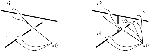
For a singular $I$ -fiber, the product $\sigma_{i}\sigma_{i}^{\prime}$ ( $\varsigma_{i}\varsigma_{i}^{\prime}$ when the fiber is in the branching locus) projects in $\pi_{1}(\mathcal{O}^{3})$ to a root of $f^{\pm 1}$ , but not in $\pi_{1}(M)$ . On the other hand, if $e_{i}$ and $e_{i+1}$ are the edges adjacent to the $i$ -th vertex, then

m_{i},m_{i}^{\prime},m_{i+1},m_{i+1}^{\prime}\in\pi_{1}(V_{i}\setminus(\Sigma_{\mathcal{O}}\cap V_{i})).

For an elliptic element $a\in\operatorname{Isom}^{+}(\mathbf{H}^{3})$ , let $\operatorname{A}(a)\subset\mathbf{H}^{3}$ denote its fixed point set (or its axis).

When the $I$ -fiber is not in the branching locus, the angle between the axis of $\rho_{0}(\sigma_{i})$ and $\rho_{0}(\sigma_{i}^{\prime})$ is

\angle(\operatorname{A}(\rho_{0}(\sigma_{i})),\operatorname{A}(\rho_{0}(\sigma_{i}^{\prime})))=\frac{p_{i}}{q_{i}}\pi

(5)

with $p_{i},q_{i}\in\mathbf{Z}$ coprime, $0<p_{i}<q_{i}$ . This rational number ${p_{i}}/{q_{i}}$ describes the singularity of the fiber, that has order $q_{i}$ . The angle of $P^{2}$ at the corresponding vertex is $\pi/q_{i}$ .

When the $I$ -fiber is in the branching locus, the angle between the axis of $\rho_{0}(\varsigma_{i})$ and $\rho_{0}(\varsigma_{i}^{\prime})$ is

\angle(\operatorname{A}(\rho_{0}(\varsigma_{i})),\operatorname{A}(\rho_{0}(\varsigma_{i}^{\prime})))=\frac{p_{i}}{2q_{i}}\vartheta_{i}

(6)

with $p_{i},q_{i}\in\mathbf{Z}$ coprime, $0<p_{i}<q_{i}$ as above and $\vartheta_{i}=2\pi/m_{i}$ is the orbifold angle, where $m_{i}\geq 2$ is the order of the branching. However, in what follows we may also consider any $0<\vartheta_{i}<2\pi$ . The angle of $P^{2}$ at the corresponding vertex is $\frac{\vartheta_{i}}{2q_{i}}$ .

Definition 7.2.

The euclidean model is the metric orbifold

E(p_{i}/q_{i})=\mathbf{R}^{3}/D_{\infty},

where $D_{\infty}$ is the infinite dihedral group generated by two rotations of order $2$ , whose axis are at distance one and have an angle (after parallel transport) equal to $\frac{p_{i}}{q_{i}}\pi$ .

Definition 7.3.

The singular euclidean model is the cone manifold

E(p_{i}/q_{i},\vartheta_{i})=\mathbf{R}^{3}(\vartheta_{i})/D_{\infty},

where $\mathbf{R}^{3}(\vartheta_{i})=\mathbf{R}^{2}(\vartheta_{i})\times\mathbf{R}$ and $\mathbf{R}^{2}(\vartheta_{i})$ is the Euclidean plane with a singular point of angle $0<\vartheta_{i}<2\pi$ . Here $D_{\infty}$ is generated by two rotations of order $2$ , with axis at distance one perpendicular to the singular axis of $\mathbf{R}^{3}(\vartheta_{i})$ , and forming an angle (after parallel transport) equal to $\frac{p_{i}}{2q_{i}}\vartheta_{i}$ .

Remark 7.4.

The orbifold $E(p_{i}/q_{i})$ and the cone manifold $E(p_{i}/q_{i},\vartheta_{i})$ have a natural fibration, that gives precisely the fibration of a neighborhood of the i-th singular vertex. This is the fibration by parallel lines of $\mathbf{R}^{3}$ , in the direction of the translation vector of the index two subgroup $\mathbf{Z}<D_{\infty}$ .

An alternative way of describing $E(p_{i}/q_{i})$ is by considering fundamental domains, cf. Figure 6. Consider a region of $\mathbf{R}^{3}$ bounded by two parallel planes at distance one. On each plane, there is a rotation axis, one for each generator, and $E(p_{i}/q_{i})$ is obtained from identifying half of each face with the other half after folding. For $E(p_{i}/q_{i},\vartheta_{i})$ , a similar fundamental domain is constructed in $\mathbf{R}^{3}(\vartheta_{i})=\mathbf{R}^{2}(\vartheta_{i})\times\mathbf{R}$ .

The fibers come from the vertical segments (say the planes are horizontal), the singular $I$ -fiber is the minimizing segment between the rotation axis. It is its soul, in the Cheeger-Gromoll sense.

Definition 7.5.

A sequence of pointed metric spaces $(X_{n},x_{n})$ converges to $(X_{\infty},x_{\infty})$ for the pointed bi-Lipschitz topology if, $\forall R>0$ and $\varepsilon>0$ , there exists $n_{0}$ such that, for $n\geq n_{0}$ , $B(x_{\infty},R)$ is $(1+\varepsilon)$ -bi-Lipschitz to a neighborhood $U\subset X_{n}$ that satisfies $B(x_{n},R-\varepsilon)\subseteq U\subseteq B(x_{n},R+\varepsilon)$ .

When constructing the developing maps in Section 9, we will use the following lemma for the transition between singular and regular $I$ -fibers:

Lemma 7.6.

Let $x_{n}$ be a sequence of points in the singular locus of $E(p_{i}/q_{i})$ . If $x_{n}\to\infty$ , then $(E(p_{i}/q_{i}),x_{n})$ converges to another euclidean model with parallel singular axis, for the pointed bi-Lipschitz topology. In addition, the distance between the axis is $q_{i}$ , the order of the singular fiber.

The same statement holds true for the cone manifold $E(p_{i}/q_{i},\vartheta_{i})$ and points in the horizontal singular locus.

Proof.

We prove it for $E(p_{i}/q_{i})$ , the proof for $E(p_{i}/q_{i},\vartheta_{i})$ being similar. The lift of the branching locus of $E(p_{i}/q_{i})$ to the universal covering (isometric to $\mathbf{R}^{3}$ ) is a countable family of lines, all of them perpendicular to a given axis that minimize the distance between any pair of the lines. From each line, we obtain the next one by a screw motion. This screw motion has axis the line perpendicular to all the lifts, translation length one and rotation angle $\frac{p_{i}}{q_{i}}\pi$ . In this way, if $x_{n}$ goes to infinity along one of the lines, the closest singular component will be parallel and at distance $q_{i}$ . Then the convergence follows easily. ∎

8 The Killing vector field

In this section we prove a result about Killing vector fields that will be used in the construction of developing maps.

Consider $P^{2}\setminus\Sigma_{P^{2}}$ the smooth part of $P^{2}$ . Via the developing map of the transversely hyperbolic foliation, the closure

\mathcal{P}=\overline{D_{0}(P^{2}\setminus\Sigma_{P^{2}})}

is a polygon in $\mathbf{H}^{2}\subset\mathbf{H}^{3}$ . Let $m_{i},m_{i}^{\prime}\in\pi_{1}(M,x_{0})$ be as in Section 7, for $i=1,\ldots,n$ . Let $\tilde{m}_{i}$ and $\tilde{m}_{i}^{\prime}$ be the corresponding paths lifted to the universal covering. We may assume that the path $D_{0}(\tilde{m}_{i})$ starts at the base point $D_{0}(\tilde{x}_{0})$ in the interior, crosses the boundary of $\mathcal{P}$ , and follows along $\rho_{0}(m_{i})(\mathcal{P})=D_{0}(m_{i}P)$ until $\rho_{0}(m_{i})(D_{0}(\tilde{x}_{0}))$ , and similarly for $m_{i}^{\prime}$ , $\sigma_{j}$ and $\sigma_{j}^{\prime}$ . Recall that $f=m_{i}(m_{i}^{\prime})^{\pm 1}$ , where the sign of the power $(m_{i}^{\prime})^{\pm 1}$ depends on the compatibility of orientations at a given axis.

By analyticity, if $\rho_{t}(f)$ is nontrivial, then there is a natural way to associate a Killing vector field $F$ to the deformation of $\rho_{t}(f)$ . Namely, as $\rho_{0}(f)=\pm\operatorname{Id}$ ,

\rho_{t}(f)=\pm\exp(t^{s}\mathfrak{f}+O(t^{s+1}))

for some $\mathfrak{f}\in\mathfrak{sl}_{2}(\mathbf{C})$ . The Killing vector field $F$ associated to the infinitesimal isometry $\mathfrak{f}$ is then

F_{x}=\lim_{t\to 0}\frac{\rho_{t}(f)(x)-x}{t^{s}}\qquad\forall x\in\mathbf{H}^{3}.

The incenter of a polygon is the point whose distance to every edge of the polygon is the same, if it exists.

The goal of this section is to prove the following:

Proposition 8.1.

The polygon $\mathcal{P}$ has an incenter and the Killing vector field $F$ is a field of infinitesimal purely loxodromic translations along an axis that meets perpendicularly $\mathcal{P}$ in its incenter. In particular $F$ is perpendicular to $\mathcal{P}$ . In addition, it has the same orientation as the fiber of the Seifert fibration of $\mathcal{O}^{3}$ restricted to the interior of $\mathcal{P}$ .

Notice that the interior of $\mathcal{P}$ is orientable because the mirror points are in $\partial\mathcal{P}$ , thus it makes sense to talk about the induced orientation of the fiber in $\mathcal{O}^{3}$ and of the Killing field on $\mathbf{H}^{3}$ .

Before proving the proposition, we need to show that $\rho_{t}(f)$ is nontrivial.

For a representation $\rho_{t}$ , a pseudodeveloping map is a $\rho_{t}$ -equivariant map $D_{t}\!:\tilde{M}\to\mathbf{H}^{3}$ , such that around the singular locus it is like the developing map around a cone singularity (ie. conical in a tubular neighborhood). This $D_{t}$ can be used to define a volume of $\rho_{t}$ [13].

Lemma 8.2.

For $\rho_{t}$ satisfying Proposition 2.1, there exists a uniform constant $C>0$ such that, for $t>0$ close to $0$ :

\operatorname{Vol}(\rho_{t})\geq Ct^{r}.

Proof.

Schläfli’s formula applied to cone manifolds [27] gives:

\operatorname{Vol}(\rho_{t})=-\frac{1}{2}\int_{0}^{t}\sum_{e}\operatorname{length}(e)d\alpha_{e},

where the sum runs over all singular edges or components. In our case, as the length is bounded below, and the cone angles are $\pi-t^{r}+O(t^{r+1})$ , the lemma is straightforward. ∎

Lemma 8.3.

For small $t>0$ , $\rho_{t}(f)$ is nontrivial.

Proof.

Seeking a contradiction, assume that $\rho_{t}(f)$ is trivial. Then, $\rho_{t}(m_{i}^{\prime})=\rho_{t}(m_{i})^{\pm 1}$ .

We first claim that for small values of $t>0$ , $\rho_{t}$ of the $i$ -th tangle group is elliptic, ie. for a tubular neighborhood $V_{i}$ of the i-th $I$ -fiber, $\rho_{t}(\pi_{1}(V_{i}\setminus(V_{i}\cap\Sigma_{\mathcal{O}})))$ is elliptic. We assume first that the singular $I$ -fiber is not in the branching locus of the orbifold. Again by contradiction, assume that the axis of $\rho_{t}(\sigma_{i})$ and $\rho_{t}(\sigma_{i}^{\prime})$ are disjoint. Then there is a minimizing segment between the axis of $\rho_{t}(\sigma_{i})$ and $\rho_{t}(\sigma_{i}^{\prime})$ , because the axis of $\rho_{0}(\sigma_{i})$ and $\rho_{0}(\sigma_{i}^{\prime})$ meet at one point with angle $\frac{\pi}{q_{i}}$ . By rescaling the hyperbolic space in such a way that the length of this segment is one, and by taking the pointed limit with base point the midpoint of this segment, we look at the limits of the axis $\operatorname{A}(\rho_{t}(\sigma_{i}))$ and $\operatorname{A}(\rho_{t}(\sigma_{i}^{\prime}))$ after rescaling: we obtain two euclidean lines at distance one and forming an angle, as in the euclidean model of Definition 7.2. In this model, the axis of the $m_{i}$ and $m_{i}^{\prime}$ are parallel but different, by Lemma 7.6. This contradicts that $\rho_{t}(m_{i}^{\prime})=\rho_{t}(m_{i})^{\pm 1}$ , and hence $\operatorname{A}(\rho_{t}(\sigma_{i}))$ and $\operatorname{A}(\rho_{t}(\sigma_{i}^{\prime}))$ meet at one point. When the singular $I$ -fiber is in the branching locus of the orbifold, then a similar argument tells that the segment between $\operatorname{A}(\rho_{t}(\varsigma_{i}))\cap\operatorname{A}(\rho_{t}(\bar{\varsigma}_{i}))$ and $\operatorname{A}(\rho_{t}(\varsigma_{i}^{\prime}))\cap\operatorname{A}(\rho_{t}(\bar{\varsigma}_{i}^{\prime}))$ has length zero.

Construct a pseudodeveloping map $D_{t}\!:\tilde{M}\to\mathbf{H}^{3}$ as follows. Start by mapping a tubular neighborhood of the singularity to a tubular neighborhood of the axis of the corresponding elements via $\rho_{t}$ . Now, since $\rho_{t}$ of the edge groups is elliptic, the singular $I$ -fiber can be mapped to a neighborhood of this point. Similarly, as $\operatorname{A}(\rho_{t}(m_{i}))=\operatorname{A}(\rho_{t}(m_{i}^{\prime}))$ , the regular $I$ -fibers can be mapped to a $\delta$ -neighborhood of the axis, for $\delta>0$ arbitrarily small. The boundary of the neighborhood of the $I$ -fibers is a torus, and since $\rho_{t}(f)$ is trivial, this torus can be deformed $\rho_{t}$ -equivariantly to a circle, in a neighborhood of radius $2\delta$ . Extend $D_{t}$ by collapsing the rest of the manifold to a disk. Thus $\rho(t)$ has arbitrary small volume, by choosing the $\delta>0$ small enough, contradicting Lemma 8.2. ∎

Recall that the Killing vector field $F$ is the corresponding field of the infinitesimal isometry $\mathfrak{f}\in\mathfrak{sl}_{2}(\mathbf{C})$ , where $\rho_{t}(f)=\pm\exp(t^{s}\mathfrak{f}+O(t^{s+1}))$ . By Lemma 8.3, $\mathfrak{f}\neq 0$ and $s$ is well defined.

Lemma 8.4.

If $\rho_{t}(f)=\exp(t^{s}\mathfrak{f}+O(t^{s+1}))$ , and $r\in\mathbf{N}$ is as in Proposition 2.1, then

s\leq r.

Proof.

By Lemma 8.2, $\operatorname{Vol}(\rho_{t})\geq Ct^{r}$ for some uniform constant $C>0$ .

On the other hand, the displacement function of $\rho_{t}(f)$ in a compact neighborhood $U$ of $\mathcal{P}$ is $\leq C_{0}t^{s}$ . In particular, the Hausdorff distance between $\operatorname{A}(\rho_{t}(m_{i}))\cap U$ and $\operatorname{A}(\rho_{t}(m_{i}^{\prime}))\cap U$ is $\leq C_{1}t^{s}$ .

We want to construct a pseudodeveloping map with volume $\leq C^{\prime}t^{s}$ . We start by constructing a developing map around the singular locus, by taking a small radius of the tube, with arbitrarily small volume, say $\leq t^{s}$ . Moreover as the Hausdorff distance between $\operatorname{A}(\rho_{t}(m_{i}))\cap U$ and $\operatorname{A}(\rho_{t}(m_{i}^{\prime}))\cap U$ is $\leq C_{1}t^{s}$ , we can develop a solid torus that is a neighborhood of the $I$ -fibers with volume $\leq C_{2}t^{s}$ , and so that the length of the fiber is $\leq 3C_{1}t^{s}$ . The exterior of this torus in $\mathcal{O}^{3}$ is a solid torus without singularity $V$ , and since the displacement function of $\rho_{t}(f)$ in $U$ is $\leq C_{0}t^{s}$ , the pseudodeveloping map can be extended to $V$ with a volume contribution $\leq C_{3}t^{s}$ . Thus, the volume of the pseudodeveloping map, and of $\rho_{t}$ , is $\leq C^{\prime}t^{s}$ . Comparing both inequalities for the volume:

Ct^{r}\leq\operatorname{Vol}(\rho_{t})\leq C^{\prime}t^{s},

for small values of $t>0$ . Thus $s\leq r$ . ∎

Before proving Proposition 8.1, we still need a further computation. Let

B:\mathfrak{sl}_{2}(\mathbf{C})\times\mathfrak{sl}_{2}(\mathbf{C})\to\mathbf{C}

denote the complex Killing form, see Appendix B. For $\mathfrak{a},\mathfrak{b}\in\mathfrak{sl}_{2}(\mathbf{C})$ ,

B(\mathfrak{a},\mathfrak{b})=\operatorname{Trace}(Ad_{\mathfrak{a}}\circ Ad_{\mathfrak{b}})=4\operatorname{Trace}(\mathfrak{a}\mathfrak{b}).

Definition 8.5.

We say that an infinitesimal isometry $\mathfrak{a}\in\mathfrak{sl}_{2}(\mathbf{C})$ has complex length $l\in\mathbf{C}$ if $\exp(t\mathfrak{a})$ has complex length $t\,l$ .

Lemma 8.6.

Let $\mathfrak{d}_{i}\in\mathfrak{sl}_{2}(\mathbf{C})$ denote infinitesimal rotation of complex length $\pi\mathbf{i}$ around the $i$ -the oriented axis of $\mathcal{P}$ . Then

B(\mathfrak{d}_{i},\mathfrak{f})=\left\{\begin{array}[]{l}0,\textrm{ if }s<r.\\ 4,\textrm{ if }s=r.\end{array}\right.

In particular $B(\mathfrak{d}_{i},\mathfrak{f})$ is independent of $i$ .

We will show later in Lemma 8.8 that only the case $B(\mathfrak{d}_{i},\mathfrak{f})=4$ occurs, in particular $s=r$ .

Proof.

We can find $\Lambda_{t},\Lambda^{\prime}_{t}\in SL_{2}(\mathbf{C})$ that depend analytically on $t^{1/2}$ , $t\in(0,\varepsilon)$ so that $\Lambda_{0}=\Lambda_{0}^{\prime}=\operatorname{Id}$ ,

\operatorname{A}(\rho_{t}(m_{i}))=\Lambda_{t}(\operatorname{A}(\rho_{0}(m_{i})))\qquad\textrm{ and }\qquad\operatorname{A}(\rho_{t}(m_{i}^{\prime}))=\Lambda_{t}^{\prime}(\operatorname{A}(\rho_{0}(m_{i}^{\prime}))).

Those matrices $\Lambda_{t}$ and $\Lambda_{t}^{\prime}$ are obtained by solving the characteristic polynomials for $\rho_{t}(m_{i})$ and $\rho_{t}(m_{i}^{\prime})$ , hence they are analytic on $t^{1/2}$ .

Assume that the axis of $\rho_{0}(m_{i})$ is $\overline{0\infty}$ in the upper half space model of $\mathbf{H}^{3}$ . If the orientations of $m_{i}$ and $m_{i}^{\prime}$ are compatible, then.

\rho_{t}(m_{i})=\pm\Lambda_{t}\begin{pmatrix}e^{i\alpha_{i}/2}&0\\ 0&e^{-i\alpha_{i}/2}\end{pmatrix}\Lambda_{t}^{-1},\quad\rho_{t}(m_{i}^{\prime})=\pm\Lambda_{t}^{\prime}\begin{pmatrix}e^{i\alpha_{i}^{\prime}/2}&0\\ 0&e^{-i\alpha_{i}^{\prime}/2}\end{pmatrix}(\Lambda_{t}^{\prime})^{-1}.

Notice that since $\rho_{0}(f)=\pm\operatorname{Id}$ , if $\rho_{t}(f)=\pm\exp(t^{s}\mathfrak{f}+O(t^{s+1}))$ , then

\Lambda_{t}^{-1}\rho_{t}(f)\Lambda_{t}=\pm\exp(t^{s}\mathfrak{f}+O(t^{s+1})),

hence we may assume $\Lambda_{t}=\operatorname{Id}$ (after replacing $\Lambda^{\prime}_{t}$ by $\Lambda_{t}^{-1}\Lambda^{\prime}_{t}$ ). Let

\Lambda_{t}^{\prime}=\begin{pmatrix}1+at^{\nu}&bt^{\nu}\\ ct^{\nu}&1-at^{\nu}\end{pmatrix}+O(t^{\nu+1/2}),

with $a,b,c\in\mathbf{C}$ , $\nu\in\frac{1}{2}\mathbf{N}$ . Since $\alpha_{i}(t)=\pi-t^{r}+O(t^{r+1})$ and $\alpha_{i}^{\prime}(t)=\pi-t^{r}+O(t^{r+1})$ ,

\rho_{t}(f)=\rho_{t}(m_{i})\rho_{t}(m_{i}^{\prime})=\pm\begin{pmatrix}-1+\mathbf{i}t^{r}&2t^{\nu}b\\ 2t^{\nu}c&-1-\mathbf{i}t^{r}\end{pmatrix}+O(t^{\min(r,\nu)+1/2}).

(7)

When $m_{i}$ and $m_{i}^{\prime}$ have opposite orientation, then

\rho_{t}(m_{i}^{\prime})=\pm\Lambda_{t}^{\prime}\begin{pmatrix}e^{-i\alpha_{i}^{\prime}/2}&0\\ 0&e^{i\alpha_{i}^{\prime}/2}\end{pmatrix}(\Lambda_{t}^{\prime})^{-1},

and since $f=m_{i}(m_{i}^{\prime})^{-1}$ , (7) also holds true.

Let $\mathfrak{d}_{i}$ be the infinitesimal rotation around the oriented axis of $\rho_{0}(m_{i})$ of complex length $\pi\mathbf{i}$ . In this model:

\mathfrak{d}_{i}=\begin{pmatrix}\mathbf{i}/2&0\\ 0&-\mathbf{i}/2\end{pmatrix}.

From (7) we distinguish two cases:

1)

If $\nu<r$ , then $s=\nu<r$ and

$\mathfrak{f}=\begin{pmatrix}0&-2b\\ -2c&0\end{pmatrix}.$ (8)
2)

If $\nu\geq r$ , then $s=r$ and

$\mathfrak{f}=\begin{pmatrix}-\mathbf{i}&-2b\\ -2c&\mathbf{i}\end{pmatrix}.$ (9)

This includes the case $\nu>r$ , with $b=c=0$ .

Then the formula follows from $B(\mathfrak{d}_{i},\mathfrak{f})=4\operatorname{Trace}(B(\mathfrak{d}_{i}\mathfrak{f}))$ . ∎

Remark 8.7.

It follows from the proof of Lemma 8.6 that the Killing vector field $F$ is perpendicular to the axis $\operatorname{A}(\rho_{0}(m_{i}))$ . This holds from Equalities (8) and (9), because in both cases the real part of the diagonal of $\mathfrak{f}$ vanishes, and the axis is $\operatorname{A}(\rho_{0}(m_{i}))=\overline{0\infty}$ .

Lemma 8.8.

$r=s$ .

Proof.

Assume that $s<r$ , hence $B(\mathfrak{f},\mathfrak{d}_{i})=0$ for each $i=1,\ldots,n$ . Using the formulas of Appendix B, we shall find a contradiction. When $\mathfrak{f}$ is non parabolic, let $\operatorname{A}(\mathfrak{f})\subset\mathbf{H}^{3}$ denote the axis of $\mathfrak{f}$ , which is the minimizing set for the norm of the Killing vector field $|F|$ . If $f$ is non parabolic, then by Proposition B.1 the complex distance between $\operatorname{A}(\mathfrak{f})$ and $\operatorname{A}(\mathfrak{d}_{i})$ is $\pm\frac{\pi}{2}\mathbf{i}$ , hence $\operatorname{A}(\mathfrak{f})$ must meet perpendicularly all edges of $\mathcal{P}$ , which is impossible. So we assume that $\mathfrak{f}$ is parabolic. In this case, Proposition B.3 tells that the point at $\infty$ fixed by $\mathfrak{f}$ is an endpoint of all (infinite) edges of $\mathcal{P}$ , which is again impossible. ∎

Proof of Proposition 8.1.

By Lemmas 8.8 and 8.6, $r=s$ and $B(\mathfrak{f},\mathfrak{d}_{i})=4$ for each $i=1,\ldots,n$ . We discuss again the possibilities for $\mathfrak{f}$ . If $\mathfrak{f}$ was parabolic, then Corollary B.5 would tell that all (infinite) edges of $\mathcal{P}$ are tangent to a given horosphere, and that their tangent vectors are parallel in this horosphere, which is again impossible. Hence we are left with the case that $\mathfrak{f}$ is nonparabolic and has an axis whose complex distance to all oriented edges of $\mathcal{P}$ is the same (by Proposition B.1).

Notice that by Remark 8.7, the Killing vector field $F$ is perpendicular to every edge of $\mathcal{P}$ . Hence, at the vertices of $\mathcal{P}$ , $F$ is perpendicular to the plane containing $\mathcal{P}$ , and since it is a Killing vector field, $F$ is perpendicular to $\mathcal{P}$ . Thus $\mathfrak{f}$ is either an infinitesimal rotation with axis coplanar to $\mathcal{P}$ or an infinitesimal translation with axis perpendicular to $\mathcal{P}$ . If $\mathfrak{f}$ is an infinitesimal rotation then by Remark B.2 (Equation 19) the complex distance between $\operatorname{A}(\mathfrak{f})$ and every oriented axis of $\mathcal{P}$ is the same, but this is impossible in a coplanar configuration. Thus $\mathfrak{f}$ is an infinitesimal translation, and its axis meets $\mathcal{P}$ perpendicularly and is equidistant to all edges of $\mathcal{P}$ .

Finally, the assertion about orientations follows from the next lemma. ∎

Lemma 8.9.

If the cone angles decrease, then the orientation of the Killing vector field $F$ is the same as the orientation of the fiber in $\mathcal{O}^{3}$ . If they increase, then it is the opposite orientation.

Proof.

By Lemma 8.2, the volume of the representation is positive, $\operatorname{Vol}(\rho_{t})>0$ for $t>0$ . On the other hand, if the orientation of the Killing vector field was the wrong one, we would be able to construct a pseudodeveloping map with negative volume, following the strategy of Lemma 8.3. ∎

Corollary 8.10.

For $t\in(0,\varepsilon)$ , $\rho_{t}(f)$ is loxodromic (ie. not elliptic nor parabolic).

Proof.

Assume first that $\rho_{0}(f)=\operatorname{Id}$ . Since $\mathfrak{f}$ is hyperbolic, then the first nonzero derivative of the trace of $\rho_{t}(f)$ is real positive, in particular for small values of $t>0$ it is not contained in $[-2,2]$ . A similar argument applies when $\rho_{0}(f)=-\operatorname{Id}$ . ∎

9 Constructing developing maps

Along this section, assume that $\rho_{t}$ , $t\in[0,\varepsilon)$ , is a path of representations that satisfies the conclusion of Proposition 2.1. The goal is to construct developing maps with holonomy $\rho_{t}$ .

We construct the developing maps in three steps. Firstly, in a neighborhood of the vertices of $P^{2}$ , that correspond to tangles of the orbifold, or singular interval fibers. Secondly, on the edges, and finally on the interior.

We start with the vertices of $P^{2}$ , ie. the tangles of $\mathcal{O}^{3}$ .

We assume for the moment that the $I$ -fiber of the $i$ -th vertex is not in the branching locus of the orbifold. (See Remark 9.5 when it is in the branching locus of the orbifold). Let $\sigma_{i}$ and $\sigma_{i}^{\prime}$ in $\pi_{1}(M)$ denote the meridians corresponding to the $i$ -th tangle, as in Section 7 (Figure 4).

Lemma 9.1.

For $t>0$ ,

\operatorname{dist}(\operatorname{A}(\rho_{t}(\sigma_{i})),\operatorname{A}(\rho_{t}(\sigma_{i}^{\prime}))>0.

Moreover, there is a shortest segment $\nu_{i}(t)$ between both axis that converges to the $i$ -th vertex of the polygon as $t\to 0^{+}.$

Proof.

By contradiction, assume that $\operatorname{dist}(\operatorname{A}(\rho_{t}(\sigma_{i})),\operatorname{A}(\rho_{t}(\sigma_{i}^{\prime})))=0$ for small values of $t>0$ . Since $\angle(\operatorname{A}(\rho_{0}(\sigma_{i})),\operatorname{A}(\rho_{0}(\sigma_{i}^{\prime}))=\pi p_{i}/q_{i}$ , $\langle\rho_{t}(\sigma_{i}),\rho_{t}(\sigma_{i}^{\prime})\rangle$ is an elliptic group that fixes a point close to the initial vertex in $\mathbf{H}^{3}$ . In particular, since $m_{i},m_{i}^{\prime}\in\langle\sigma_{i},\sigma_{i}^{\prime}\rangle$ , $\rho_{t}(f^{\pm 1})=\rho_{t}(m_{i})\,\rho_{t}(m_{i}^{\prime})^{\pm 1}$ is either trivial or elliptic, which contradicts Corollary 8.10.

The existence of the shortest segment $\nu_{i}(t)$ comes from the fact that $\operatorname{A}(\rho_{0}(\sigma_{i}))$ and $\operatorname{A}(\rho_{0}(\sigma_{i}^{\prime}))$ meet at one point with angle $\pi\frac{p_{i}}{q_{i}}$ , so the distance function between both axis is a proper convex function on $\operatorname{A}(\rho_{0}(\sigma_{i}))\times\operatorname{A}(\rho_{0}(\sigma_{i}^{\prime}))$ and has a minimum. Therefore, for small $t>0$ it is also a proper convex function on $\operatorname{A}(\rho_{t}(\sigma_{i}))\times\operatorname{A}(\rho_{t}(\sigma_{i}^{\prime}))$ and has a minimum. ∎

The idea now is to construct a double roof ${\mathcal{R}}_{i}(t)$ around $\nu_{i}(t)$ as follows. Consider an embedding of both axis $\operatorname{A}(\rho_{t}(\sigma_{i}))$ and $\operatorname{A}(\rho_{t}(\sigma_{i}^{\prime}))$ and the common perpendicular $\nu_{i}(t)$ in $\mathbf{H}^{3}$ . Now consider two sectors, one with axis $\operatorname{A}(\rho_{t}(\sigma_{i}))$ and angle $\alpha_{i}(t)$ , another one with axis $\operatorname{A}(\rho_{t}(\sigma_{i}^{\prime}))$ and angle $\alpha_{i}^{\prime}(t)$ . (Here $\alpha_{i}(t)$ and $\alpha_{i}^{\prime}(t)$ are the respective rotation angles of $\rho_{t}(\sigma_{i})$ and $\rho_{t}(\sigma_{i}^{\prime})$ ). Choose the sectors so that $\nu_{i}(t)$ is bisector to both of them, and consider the intersection (Figure 7).

The boundary of these sectors may intersect. Let $r_{i}(t)>0$ be the maximal radius such that the tubular neighborhood $\mathcal{N}_{r_{i}(t)}(\nu_{i}(t))$ does not meet the intersection of the sides of the sectors. We denote ${\mathcal{R}}_{i}(t)=\mathcal{N}_{r_{i}(t)/2}(\nu_{i}(t))$ the tubular neighborhood of $\nu_{i}(t)$ in this double roof. Notice that possibly $r_{i}(t)\to 0$ as $t\to 0^{+}$ , but:

Lemma 9.2.

\lim_{t\to 0^{+}}\frac{r_{i}(t)}{|\nu_{i}(t)|}=+\infty.

Proof.

We cut the double roof along the hyperplane perpendicular to $\nu_{i}(t)$ that contains its midpoint, and consider each roof separately. We bound below the distance from $\nu_{i}(t)$ to the intersection of each piece of the roof to this hyperplane, and it suffices to discuss the argument for one of the edges, say $\sigma_{i}$ . Let $\alpha_{i}(t)$ denote the cone angle, which is the angle of the roof. By comparison with the euclidean right triangle (Figure 8):

\frac{r_{i}(t)}{|\nu_{i}(t)|/2}\geq\tan\frac{\alpha_{i}(t)}{2}\to\infty\quad\textrm{ as }t\to 0^{+},

because $\alpha_{i}(0)=\pi$ . ∎

Let $x_{i}(t)$ denote the midpoint of $\nu_{i}(t)$ . Let $\overline{\mathcal{R}}_{i}(t)$ be the result of identifying the sides of each roof of ${\mathcal{R}}_{i}(t)$ by a rotation around its edge, so that the edges become interior points.

From Lemma 9.2, we get:

Corollary 9.3.

For the pointed bi-Lipschitz topology:

\lim_{t\to 0^{+}}\frac{1}{|\nu_{i}(t)|}(\overline{\mathcal{R}}_{i}(t),x_{i}(t))=(E(p_{i}/q_{i}),x_{\infty}).

Next corollary deals with points of $\overline{\mathcal{R}}_{i}(t)$ away from the center.

Corollary 9.4.

There exist $R_{0}>0$ and $t_{0}>0$ such that for $0<t\leq t_{0}$ and $x\in\overline{\mathcal{R}}_{i}(t)$ that it is singular and $R_{0}|\nu_{i}(t)|\leq d(x,x_{i}(t))<\frac{1}{2}r_{i}(t)$ , the following hold. Let ${{\delta}}(x)$ be the distance between $x$ and the other singular component. Then the rescaled ball

\frac{1}{{{\delta}}(x)}B(x,10{{\delta}}(x))

is $3/2$ -bi-Lipschitz to the corresponding ball in $E(0)$ .

Proof.

By Corollary 9.3, it is sufficient to prove it for the euclidean models $E(p_{i}/q_{i})$ . Then the corollary follows from Lemma 7.6. ∎

Remark 9.5.

When the $I$ -fiber of the $i$ -th vertex is in the branching locus of the orbifold, then one needs to consider the double roofs $\mathcal{R}_{i}(t)$ and the corresponding neighborhoods $\overline{\mathcal{R}_{i}(t)}$ with a singular core $\nu_{i}(t)$ of cone angle $\vartheta_{i}$ . Lemma 9.2 and Corollaries 9.3 and 9.4 apply in this case.

Next we deal with the edges of $P^{2}$ . We shall construct locally the hyperbolic structures in pieces $\overline{\mathcal{S}}(q)$ and study its behavior and compatibility in Corollary 9.8 and Lemma 9.9. Before that, we need few technical results about the edges $\operatorname{A}(\rho_{t}(m_{i}))$ and $\operatorname{A}(\rho_{t}(m_{i}^{\prime}))$ .

To simplify notation, set $i=1$ . The endpoints of the segment $e_{1}$ of $\mathcal{P}^{2}$ at time $t=0$ are $v_{1}$ and $v_{2}$ . But for $t>0$ , we consider two segments $e_{1}(t)$ and $e_{1}^{\prime}(t)$ that are contained in $\operatorname{A}(\rho_{t}(m_{1}))$ and $\operatorname{A}(\rho_{t}(m_{1}^{\prime}))$ , respectively, and whose endpoints are given by the $\sigma$ ’s or $\varsigma$ ’s: ie. the endpoints of the corresponding conjugates of $\nu_{1}(t)$ and $\nu_{2}(t)$ .

Let $p_{1}(t)$ and $p_{2}(t)$ denote the endpoints of $e_{1}(t)$ . For $q\in e_{1}(t)$ , let $q^{\prime}\in\operatorname{A}(\rho_{t}(m_{1}^{\prime}))$ be the point that realizes the distance between $q$ and $\operatorname{A}(\rho_{t}(m_{1}^{\prime}))$ (cf. Fig. 9). Define, for $q\in e_{1}$ :

{{\delta}}_{t}(q)=d(q,q^{\prime})=d(q,\operatorname{A}(\rho_{t}(m_{1}^{\prime}))).

Lemma 9.6.

Let $q\in e_{1}(t)$ and $q^{\prime}\in\operatorname{A}(\rho_{t}(m^{\prime}_{1}))$ be as above.

1.

The distance ${{\delta}}_{t}(q)=d(q,q^{\prime})$ converges to zero uniformly on $q\in e_{1}(t)$ :

$\lim_{t\to 0^{+}}\sup_{q\in e_{1}(t)}{{\delta}}_{t}(q)=0$
2.

Let $v_{q,t}\in T_{q}\mathbf{H}^{3}$ be the parallel transport of the tangent vector to $e_{1}^{\prime}(t)$ along the segment $\overline{q^{\prime}q}$ . Then

$\lim_{t\to 0^{+}}\sup_{q\in e_{1}(t)}\angle_{q}e_{1}(t)v_{q,t}=0$
3.

Let $R_{0}>0$ be as in Corollary 9.4. There exists $t_{0}>0$ such that, for $0<t<t_{0}$ , $q\in e_{1}(t)$ satisfies $d(q,p_{1}(t))>R_{0}\,|\nu_{1}(t)|$ and $d(q,p_{2}(t))>R_{0}\,|\nu_{2}(t)|$ , then:

$q^{\prime}\in e_{1}^{\prime}(t).$

Proof.

By convexity of the distance function in hyperbolic space, we have, for $q\in e_{1}(t)$ :

{{\delta}}_{t}(q)\leq\max\{{{\delta}}_{t}(p_{1}(t)),{{\delta}}_{t}(p_{2}(t))\},

(10)

because $p_{1}(t)$ and $p_{2}(t)$ are the endpoints of $e_{1}(t)$ . This proves Assertion 1 of the lemma.

In order to prove Assertion 3, if $d(q,p_{1}(t))=R_{0}\,|\nu_{1}(t)|$ or if $d(q,p_{2}(t))=R_{0}\,|\nu_{2}(t)|$ , then the assertion holds true for these $q$ , because of Corollary 9.4. As those $q$ are extremal, for other $q$ the assertion follows from Equation (10) and elementary arguments.

Next we prove Assertion 2. Up to permuting $p_{1}$ with $p_{2}$ , we may assume that $d(q,p_{1}(t))>\frac{1}{3}|e_{1}(0)|$ , where $|e_{1}(0)|$ denotes the length of $e_{1}(0)$ . Let $\beta_{q}(t)$ be the angle between $v_{q,t}$ and $e_{1}(t)$ . By the triangle inequality in spherical space, the angle $\beta_{q}(t)$ satisfies: $0\leq\beta_{q}(t)\leq\beta_{1}+\beta_{2}$ , where $\beta_{1}$ is the angle between $v_{q,t}$ and $qp_{1}^{\prime}$ , $\beta_{2}$ is the angle between $qp_{1}^{\prime}$ and $qp_{1}\subset e_{1}(t)\subset\operatorname{A}(\rho_{t}(m_{1}))$ , and $p_{1}^{\prime}\in\operatorname{A}(\rho_{t}(m_{1}^{\prime}))$ realizes $d(p_{1},\operatorname{A}(\rho_{t}(m_{1}^{\prime})))=d(p_{1},p_{1}^{\prime})$ , cf. Figure 10.

Let $p^{\prime\prime}\in\operatorname{A}(\rho_{t}(m_{1}))$ realize the distance from $p_{1}^{\prime}$ to $\operatorname{A}(\rho_{t}(m_{1}))$ , so that $q$ , $p_{1}^{\prime}$ and $p^{\prime\prime}$ form a triangle with angles $\beta_{2}$ at $q$ , and $\pi/2$ at $p^{\prime\prime}$ . Then

\tan\beta_{2}=\frac{\tanh d(p_{1}^{\prime},p^{\prime\prime})}{\sinh d(q,p^{\prime\prime})}\leq\frac{\tanh d(p_{1}^{\prime},p^{\prime\prime})}{\sinh(\frac{1}{3}|e_{1}(0)|-d(p_{1},p^{\prime\prime}))}

which converges to zero uniformly on $q$ . Consider now the triangle $q$ , $q^{\prime}$ and $p_{1}^{\prime}$ . By the same argument as before the angle $\beta_{3}$ of this triangle at $p_{1}^{\prime}$ converges to zero. The angles of the triangle satisfy:

(\frac{\pi}{2}-\beta_{1})+\frac{\pi}{2}+\beta_{3}=\pi-\textrm{Area}(qq^{\prime}p_{1}^{\prime}).

In addition, the area of this triangle converges to zero uniformly on $q$ , by Assertion 1 of the lemma. Thus

\beta_{1}=\beta_{3}+\textrm{Area}(qq^{\prime}p_{1}^{\prime})\to 0,\qquad\textrm{ uniformly on }q.

∎

We define, for $0<t<t_{0}$ as in Assertion 3 of Lemma 9.6:

\hat{e}_{1}(t)=\left\{q\in e_{1}(t)\mid d(q,p_{1}(t))\geq R_{0}\,|\nu_{1}(t)|\textrm{ and }d(q,p_{2}(t))\geq R_{0}\,|\nu_{2}(t)|\right\}.

Using also Lemma 9.6, construct a double roof from the segment between $q$ and $q^{\prime}$ , with edges determined by $\operatorname{A}(\rho_{t}(m_{1}))$ and $\operatorname{A}(\rho_{t}(m_{1}^{\prime}))$ , and with dihedral angles the respective rotation angles of $\rho_{t}(m_{1})$ and $\rho_{t}(m_{1}^{\prime})$ , $\alpha_{1}(t)$ and $\alpha_{1}^{\prime}(t)$ , as before. Let ${\mathcal{S}}(q,t)=B(q,s(q,t)/2)$ be the ball in this double roof, with $s(q,t)$ maximal such that the sides of the roof do not meet. As in Lemma 9.2:

Lemma 9.7.

\lim_{t\to 0^{+}}\frac{s(q,t)}{d(q,q^{\prime})}=+\infty

uniformly on $q\in\hat{e}_{1}(t)$ .

The proof of this limit is the same as Lemma 9.2, using the uniform limits of Lemma 9.6.

Identifying the sides of ${\mathcal{S}}(q,t)$ by the rotations corresponding to its edges, we obtain $\overline{\mathcal{S}}(q,t)$ . From Lemmas 9.7 and 9.6, we get:

Corollary 9.8.

For any choice of $q(t)\in\hat{e}_{1}(t)$ and for the pointed bi-Lipschitz topology:

\lim_{t\to 0^{+}}\frac{1}{{{\delta}}_{t}(q)}(\overline{\mathcal{S}}(q,t),q(t))=(E(0),q_{\infty}),

uniformly on $q$ .

Recall that ${{\delta}}_{t}(q)=d(q,q^{\prime})=d(q,\operatorname{A}(\rho_{t}(m^{\prime}_{i})))$ .

Lemma 9.9.

Let $r\in\overline{\mathcal{S}}(q,t)$ belong to the same connected component of the singular locus as $q$ . Let $r^{\prime}$ and $q^{\prime}$ be the corresponding closest points in the other components. If $d(q,r)\leq 10{{\delta}}_{t}(q)$ , then the angle between $qq^{\prime}$ and $rr^{\prime}$ after parallel transport (along any of both singular components) is $\leq\gamma(t)$ , for some uniform $\gamma(t)\to 0$ .

This lemma follows easily from the estimates of Lemma 9.6 and elementary trigonometric arguments.

Proposition 9.10.

Let $\rho_{t}$ be as in Proposition 2.1. There exists $\varepsilon>0$ such that for $t\in(0,\varepsilon)$ there exists $D_{t}\!:\!\tilde{M}\to\mathbf{H}^{3}$ the developing map of a cone structure on $(|\mathcal{O}^{3}|,\Sigma_{\mathcal{O}^{3}})$ with holonomy $\rho_{t}$ . In addition, when $t\to 0$ , $D_{t}$ converges to $D_{0}$ , the developing map of the transverse hyperbolic foliation.

Proof.

Let $0<t<t_{0}$ , where $t_{0}>0$ is as in Assertion 3 of Lemma 9.6. The edge $\hat{e}_{1}(t)$ is covered by balls $B(q,2{{\delta}}_{t}(q))$ . Choose a finite covering of such balls, with centers $q$ in $\hat{e}_{1}(t)$ . We claim that the model $\overline{\mathcal{S}}(q,t)$ of each ball matches with the next one: this is a consequence of Lemma 9.9, because the segments between $q$ and the opposite singular edge vary continuously with $q$ , and they are almost parallel (the difference with the parallel transport is uniformly small in $B(q,10{{\delta}}_{t}(q))$ ). Notice also that the position of the singular edges is determined by the isometries $\rho_{t}(m_{1})$ and $\rho_{t}(m^{\prime}_{1})$ . This gives a metric structure for a neighborhood of the edges.

By Lemma 7.6, when $q\in\partial\hat{e}_{1}(t)$ , then the $\overline{\mathcal{S}}(q,t)$ match with the corresponding $\overline{\mathcal{R}}_{i}(t)$ . In this way we put a geometric structure on a solid torus that contains the singular locus, made of the union of 0-cells (the $\overline{\mathcal{R}}_{i}(t)$ for the singular vertices of the polygon) and $1$ -cells (the union of $\overline{\mathcal{S}}(q,t)$ for the edges of the polygon). Let $D_{t}$ be the corresponding developing map of this solid torus that contains the singular locus.

Notice that the orientation is globally preserved, by Proposition 8.1, and because it depends on the displacement of $\rho_{t}(f)$ .

Recall that we assume that there is no singular fiber in the interior of the orbifold. Look at the 2-torus that bounds the previous tubular neighborhood of the singularity. Now the developing map of the universal covering of the 2-torus factors to a map from the 2-torus to the hyperbolic solid torus $\mathbf{H}^{3}/\rho_{t}(f)$ , ( $\rho_{t}(f)$ is hyperbolic by Corollary 8.10). By Proposition 8.1, this map is injective on the intersection of the $2$ -torus and each model $\overline{\mathcal{S}}(q,t)$ and $\overline{\mathcal{R}}_{i}(t)$ . In addition, the models are either far apart or their intersection is well understood, by the previous discussion, hence it is an embedding of the torus.

Since it is not contained in a ball, this 2-torus must bound a solid torus in $\mathbf{H}^{3}/\rho_{t}(f)$ , with meridian the curve that has trivial holonomy. This $2$ torus is fibered over a curve that converges to the singular locus. Thus we extend $D_{t}$ to the universal covering of the corresponding solid torus $V$ in the smooth part of $\mathcal{O}^{3}$ . The map $D_{t}$ restricted to each compact subset of $\partial\tilde{V}$ converges to $\partial\mathcal{P}$ , coherently with the fibration. Then we choose $D_{t}$ so that restricted to compact subsets of $\tilde{V}$ converges to the $D_{0}$ . ∎

10 Cone manifolds with geometry $\widetilde{SL_{2}(\mathbf{R})}$ and $\mathbf{H}^{2}\times\mathbf{R}$

Before explaining the proof of Theorem 1.2, we give a result about cone manifolds with those fibered geometries, just for the statement of the theorem.

As in the introduction, let $\mathcal{O}^{3}$ be an orbifold fibering over a polygonal orbifold $P^{2}$ with mirror boundary and corners. We assume that $P^{2}$ has no cone point in the interior, to simplify. We will relax the hyperbolicity condition for the orbifold $P^{2}$ by adding cone singularities at the $I$ -fibers. Choose $n$ $I$ -fibers of $\mathcal{O}$ ,

\{f_{1},\ldots,f_{n}\}

that include all singular $I$ -fibers. Let $q_{1},\ldots,q_{n}\in\mathbf{N}$ denote their respective indices in the fibration. In particular $q_{i}=1$ if and only if $f_{i}$ is a regular fiber. Fix angles $\vartheta_{1},\ldots,\vartheta_{n}\in(0,2\pi]$ so that

\vartheta_{i}/q_{i}\leq\pi,

for $i=1,\ldots,n$ . We impose also the following condition

\sum_{i=1}^{n}(\pi-\vartheta_{i}/(2q_{i}))>2\pi

this implies that the polygon $Q$ with angles $\vartheta_{i}/(2q_{i})$ is hyperbolic.

Proposition 10.1.

Given a hyperbolic structure on $Q$ , there exists a cone manifold $C(\pi)$ with geometry $\widetilde{SL_{2}(\mathbf{R})}$ or $\mathbf{H}^{2}\times\mathbf{R}$ , with the same underlying space as $\mathcal{O}^{3}$ , $\Sigma_{C(\pi)}^{Hor}=\Sigma_{\mathcal{O}^{3}}^{Hor}$ , $\Sigma_{C(\pi)}^{Vert}\subseteq f_{1}\cup\cdots\cup f_{n}$ , and respective vertical cone angles $\vartheta_{1},\ldots,\vartheta_{n}$ , and fibered over $Q$ .

In addition, every cone manifold with geometry $\widetilde{SL_{2}(\mathbf{R})}$ or $\mathbf{H}^{2}\times\mathbf{R}$ with vertical angles $\leq 2\pi$ and with space of fibers a polygon with angles $\leq\pi/2$ is obtained in this way.

Since both geometries $\widetilde{SL_{2}(\mathbf{R})}$ and $\mathbf{H}^{2}\times\mathbf{R}$ are fibered, for a cone manifold with this geometry there is a vertical and a horizontal singular locus, and the horizontal cone angle is always $\pi$ .

In the statement, a fiber $f_{i}$ is in the singular locus of the cone manifold if and only if $\vartheta_{i}<2\pi$ .

Proof.

If the angles are $\vartheta_{i}=2\pi/n_{i}$ , then $C(\pi)$ is an orbifold and this is consequence of the geometrization of Seifert fibered orbifolds (see [5, Prop. 2.13]).

For the general case, we decrease the $\vartheta_{i}$ to some $\pi/n_{i}$ and we apply a deformation argument. When the Euler number of the fibration is zero, then the geometry of the orbifold involved is $\mathbf{H}^{2}\times\mathbf{R}$ , and the geometric structure on $C(\pi)$ is deformed by deforming the basis. Otherwise, the geometric structure is $\widetilde{SL_{2}(\mathbf{R})}$ . Let $\tilde{\mathcal{O}}^{3}$ be the orientation covering of $\mathcal{O}^{3}$ , so that there is an orientation reversing involution $\tau:\tilde{\mathcal{O}}^{3}\to\mathcal{O}^{3}$ such that $\tilde{\mathcal{O}}^{3}/\tau=\mathcal{O}^{3}$ and $\textrm{Fix}(\tau)=\Sigma_{\mathcal{O}^{3}}^{Hor}$ . The orbifold $\tilde{\mathcal{O}}^{3}$ is Seifert fibered, all leaves are circles and the space of leaves is $\tilde{Q}$ , the sphere with $n$ cone points that is union of $Q$ and the mirror image of $Q$ along the boundary. The hyperbolic structure on the polygon $Q$ induces a hyperbolic structure on the cone manifold $\tilde{Q}$ .

Let $N=\mathcal{O}^{3}\setminus\mathcal{N}(\tilde{f}_{1}\cup\cdots\cup\tilde{f}_{n})\cong F\times S^{1}$ , where $F$ is a planar surface with $n$ boundary components. We first describe the holonomy representation of $N$ . Let $a_{1},\ldots,a_{n}\in\pi_{1}(F)$ denote the peripheral elements so that

\pi_{1}(F)=\langle a_{1},\ldots,a_{n}\mid a_{1}\cdots a_{n}=1\rangle.

Let $f$ be the generator of $\pi_{1}(S^{1})$ . The meridian of $\tilde{f}_{i}$ is the curve $f^{p_{i}}a_{i}^{q_{i}}$ , where $q_{i}\geq 1$ is the index of the singular fiber (regular when $q_{i}=1$ ).

Recall that the identity component of the isometry group of $\widetilde{SL_{2}(\mathbf{R})}$ is

\widetilde{SL_{2}(\mathbf{R})}\times_{\mathbf{Z}}\mathbf{R},

where $\widetilde{SL_{2}(\mathbf{R})}$ acts on itself by left multiplication and $\mathbf{R}$ is the universal covering of $SO(2)$ , the stabilizer of a point acting on itself by right multiplication of its inverse. For a representation $\rho$ in $\widetilde{SL_{2}(\mathbf{R})}\times_{\mathbf{Z}}\mathbf{R}$ , we denote by $\rho_{l}$ the projection to $PSL_{2}(\mathbf{R})$ and $\rho_{r}$ the projection to $SO(2)=\mathbf{R}/\mathbf{Z}$ . Notice that $\rho_{l}(f)=Id$ , because $PSL_{2}(\mathbf{R})$ has no center. On the other hand, for $\rho(f^{p_{i}}a_{i}^{q_{i}})$ to be a rotation of angle $\vartheta_{i}$ , working in $\mathbf{R}/2\pi\mathbf{Z}$ , we must have

p_{i}\rho_{r}(f)+q_{i}\rho_{r}(a_{i})=\vartheta_{i}\textrm{ in }\mathbf{R}/2\pi\mathbf{Z},\qquad\textrm{ for }i=1,\ldots,n.

(11)

Combining this with

\rho_{r}(a_{1})+\cdots+\rho_{r}(a_{n})=0\textrm{ in }\mathbf{R}/2\pi\mathbf{Z},

(12)

it follows that $\rho_{r}(f)$ and $\rho_{r}(a_{i})$ are locally uniquely determined in $\mathbf{R}$ , because the Euler number does not vanish:

\frac{p_{1}}{q_{1}}+\cdots+\frac{p_{n}}{q_{n}}\neq 0.

The reason is that this Euler number is the determinant of the matrix associated to the linear system (11) and (12).

Now we describe the deformation argument. By changing the angles and the hyperbolic structure of $Q$ , Equations (11) and (12) imply that we can deform the representation of $\pi_{1}(N)$ in $\widetilde{SL_{2}(\mathbf{R})}\times_{\mathbf{Z}}\mathbf{R}$ , in such a way that the meridians go to the rotation of the expected angle, this gives a $\widetilde{SL_{2}(\mathbf{R})}$ cone structure on $\tilde{\mathcal{O}}^{3}$ with the deformed cone angles on the $\tilde{f}_{i}$ . Moreover, since the solution to (11) and (12) is localy unique and the metric structure in $\tilde{Q}$ is invariant by the involution, $\tau$ is homotopic to the isometry. By applying Tollefson’s theorem to $N\cong F\times S^{1}$ , $\tau$ is conjugate to an isometry, giving the singular structure on $\mathcal{O}^{3}$ . This proves openness for the deformation. For closedness, we need to show that $\rho(f)$ will not become trivial. By contradiction, assume that $\rho(f)=0$ , then by (11) $\rho_{r}(a_{i})=\vartheta_{i}/q_{i}$ $\mod 2\pi\mathbf{Z}$ and by (12) $\sum\vartheta_{i}/q_{i}\in 2\pi\mathbf{Z}$ . Then we have to look carefully at the determinations in the universal covering $\widetilde{SL_{2}(\mathbf{R})}\times\mathbf{R}$ . Choose a lift of $\rho$ such that $\tilde{\rho}_{r}(a_{i})=\vartheta_{i}/q_{i}\in(0,2\pi)$ . Then, by a deformation argument and viewing the Euclidean case as a limit case, we get that $\tilde{\rho}_{l}(a_{1}\cdots a_{n})$ is a lift of a rotation of angle $2\pi(n-2)$ . On the other hand $\tilde{\rho}_{r}(a_{1}\cdots a_{n})$ lifts to $\sum\vartheta_{i}/q_{i}\in\mathbf{R}$ , but $\sum\vartheta_{i}/q_{i}<2\pi(n-2)$ , hence $\tilde{\rho}(a_{1}\cdots a_{k})$ cannot be the lift or a trivial element in in $\widetilde{SL_{2}(\mathbf{R})}\times_{\mathbf{Z}}\mathbf{R}$ , which leads to contradiction. ∎

Let us explain now how to adapt the proof of Theorem 1.1 to Theorem 1.2.

We use the analogue results of Section 5 to construct a curve of representations when all $\vartheta_{i}<2\pi$ . When some $\vartheta_{i}=2\pi$ , then we require the analogue deformation argument of Section 6.

The arguments of Section 5 work exactly the same, just by replacing the vector $(1,\ldots,1)$ by $(w_{1},\ldots,w_{n},w_{1}^{\prime},\ldots,w_{n}^{\prime})$ .

In Section 6 one has to work with real analytic sets instead of algebraic ones, but all results apply. Namely, Sullivan’s local Euler characteristic theorem in the proof of Corollary 6.4 is already stated for real analytic sets.

The required result on the Teichmüller space is Corollary A.6.

Regarding the construction of developing maps, Section 8 and Section 9 apply with no changes.

11 An example

Let $\mathcal{O}^{3}$ denote the orbifold with underlying space $S^{3}$ and singular locus the Whitehead link. Assume that the respective labels in the singular components are $n>4$ and $2$ . This orbifold is Seifert fibered: the component with label $n>4$ is a fiber, and the one with label $2$ is the union of mirror points of the $I$ -fibers, and projects to mirror points of $P^{2}$ . The base of the Seifert fibration is a one-edged polygonal orbifold, with a single corner, and its interior contains a cone point with label $n$ , corresponding to the singular component that is also a fiber. The angle at the corner is $\pi/2$ , cf. Figure 11.

In our proof of Theorem 1.1 we work with the $n$ -th branched covering (thus $P^{2}$ lifts to the regular $n$ -sided right-angled polygon), but for explicit computations it is easier to work in $\mathcal{O}^{3}$ instead of its covering.

The smooth part of $\mathcal{O}^{3}$ is $M=\mathcal{O}^{3}\setminus\Sigma_{\mathcal{O}^{3}}$ , the complement of the Whitehead link in $S^{3}$ . If $a,b\in\pi_{1}M$ are meridians around the two components of $\Sigma$ , the fundamental group has the following presentation, cf. [21]:

\pi_{1}(M)=\langle a,b\,|\,awa^{-1}w^{-1}\rangle

with $w=bab^{-1}a^{-1}b^{-1}ab$ . The $SL_{2}(\mathbf{C})$ -character variety of $M$ has been computed by [21]. Here we follow the exposition from [28]. Namely, after identifying $X(M)$ with the image of the map

\begin{array}[]{rl}X(M)&\rightarrow\mathbf{C}^{3}\\ \chi&\mapsto(\chi(a),\chi(b),\chi(ab))\end{array}

in $\mathbf{C}^{3}$ , it is

X(M)=\{(x,y,z)\in\mathbf{C}^{3}\mid p(x,y,z)\cdot q(x,y,z)=0\}

with

p(x,y,z)=xy-(x^{2}+y^{2}-2)z+xyz^{2}-z^{3}

and

q(x,y,z)=x^{2}+y^{2}+z^{2}-xyz-4\,.

Again by [21], $q=0$ corresponds to the abelian characters and $p=0$ is the closure of the set of irreducible characters.

We work with the subvariety $y=\pm 2\cos(\pi/n)$ , with $n>4$ . The holonomies of the deformations of Proposition 2.1 are obtained by taking $x=\pm 2\cos(\alpha/2)$ , for $\alpha=\pi-t$ close to $\pi$ .

The point of the initial holonomy $\chi_{0}$ has coordinates

x=0,\ y=\pm 2\cos(\pi/n)\textrm{ and }z=\pm\sqrt{4\cos^{2}(\pi/n)-2}\in\mathbf{i}\mathbf{R}.

The sign ambiguity comes from different lifts to $SL_{2}(\mathbf{C})$ . Since $n>4$ ,

\frac{\partial p}{\partial z}(\chi_{0})\neq 0.

Hence, by the implicit function theorem, $x$ is a local parameter of the variety

p(x,\pm 2\cos(\pi/n),z)=0

around $\chi_{0}$ . In particular $\alpha=\pi-t$ is a local parameter of our deformation space. Recall that changing the sign of $t$ corresponds to changing the orientation.

This example was the conjectural picture for a piece of the boundary of the moduli space of hyperbolic cone structures of [28].

Other regular or singular Dehn fillings on the same component of the Whitehead link give a Seifert fibered orbifold with the same base. Here we just described the $1/0$ -Dehn filling with singular core with ramification $n\geq 5$ , but we can also consider the $p/q$ -Dehn filling with $p\geq 1$ either with regular core ( $n=1$ ) or with singular core of ramification $n\geq 2$ . The base is the same orbifold, and the cone point has label $p\,n$ . So the base is hyperbolic when $p\,n>4$ . Similar explicit computations of the variety of characters can be made, but they are more involved.

Appendix A Appendix: Earthquakes and polygons

We are in the setting of Lemma 6.2. Thus, assuming that $P^{2}$ is a polygon with cone angles $\leq\vartheta_{0}/2<\pi/2$ , we take its double $C$ , which is a cone manifold with underlying space a sphere, and singular locus $n$ points of cone angle $\leq\vartheta_{0}<\pi$ .

We follow the work of Bonsante and Schlenker in [8] about earthquakes for closed cone manifolds with cone angles $<\pi$ .

The Teichmüller space of $C$ is denoted by $\mathcal{T}(C)$ , and we assume that cone angles are fixed. Let $\mathcal{ML}(C)$ and $\mathcal{PML}(C)$ denote the spaces of measured and projectively measured geodesic laminations on the smooth part of $C$ . Thus $\mathcal{ML}(C)\cong\mathbf{R}^{2n-6}$ and $\mathcal{PML}(C)\cong S^{2n-7}$ . Lemma 2.2 of [8] proves that any lamination of $C$ can be realized by a geodesic lamination. The main result of [8] for our purposes is the earthquake theorem for cone manifolds with cone angles $<\pi$ :

Theorem A.1 ([8]).

For any $S\in\mathcal{T}(C)$ , the map

	$\displaystyle\mathcal{ML}(C)$	$\displaystyle\to$	$\displaystyle\mathcal{T}(C)$
	$\displaystyle\lambda$	$\displaystyle\mapsto$	$\displaystyle E_{\lambda}^{l}(S)$

is a homeomorphism, where $E_{\lambda}^{l}$ denotes the left earthquake of $S$ along $\lambda\in\mathcal{ML}(C)$ .

We also require a version of Wolpert’s formulas [35] in our setting, namely for the lengths of the segments between cone points. Let $\sigma$ denote a geodesic segment of $C$ between two cone points. The perimeter we are interested in is the addition of lengths of such geodesic segments. The length of $\sigma$ is denoted by $|\sigma|$ .

Lemma A.2.

Let $S\in\mathcal{T}(C)$ , $\lambda\in\mathcal{ML}(C)$ and $\sigma$ a geodesic segment between two cone points. For the earthquake deformation $E_{t\lambda}^{l}(S)$ , $t\in\mathbf{R}_{+}$ :

(1)

$\frac{\partial|\sigma|}{\partial t}=\int_{\lambda}\cos\theta$ .
(2)

$\frac{\partial^{2}|\sigma|}{\partial t^{2}}\geq c\langle\lambda,\sigma\rangle^{2}$ , for some uniform $c>0$ .

Here $\theta$ denotes the angle from $\lambda$ to $\sigma$ measured counterclockwise at each intersection point, $\int_{\lambda}\cos\theta$ means the integral of the cosine of this angle on the intersection between $\sigma$ and $\lambda$ along the transverse measure of $\lambda$ , and

\langle\lambda,\sigma\rangle=\int_{\lambda}\chi_{\sigma}

is the intersection between $\lambda$ and $\sigma$ (which is the integral of the characteristic function of $\sigma$ along the transverse measure of $\lambda$ ).

To prove this lemma we use the density of weighted multicurves in $\mathcal{ML}(C)$ and reduce to the following computation:

Lemma A.3 (Wolpert’s formulas).

Let $S\in\mathcal{T}(C)$ , $\lambda\in\mathcal{ML}(C)$ and $\sigma$ a geodesic segment between two cone points. For the earthquake deformation $E_{t\lambda}^{l}(S)$ , $t\in\mathbf{R}_{+}$ :

(1)

Let $\lambda$ be a simple closed curve. Then $\frac{\partial|\sigma|}{\partial t}=\int_{\lambda}\cos\theta$ .

(2)

Let $\lambda=\sum m_{i}\lambda_{i}$ , be a weighted multicurve, with $\lambda_{i}$ disjoint simple closed curves and $m_{i}\in\mathbf{R}_{+}$ . Then

\frac{\partial^{2}|\sigma|}{\partial t^{2}}=\sum_{ij}m_{i}m_{j}\sum_{(p,q)\in(\sigma\cap\lambda_{i})\times(\sigma\cap\lambda_{j})}\frac{\cosh|\sigma_{pq}^{+}|\cosh|\sigma_{pq}^{-}|}{\sinh{|\sigma|}}\sin\theta_{p}\sin\theta_{q}

where $\sigma_{pq}^{+}$ and $\sigma_{pq}^{-}$ are the two components of $\sigma\setminus\overline{pq}$ , and $\theta_{p}$ and $\theta_{q}$ are the angles at the corresponding intersection points.

Lemma A.3(1) implies Lemma A.2(1) by density of multicurves in $\mathcal{ML}(C)$ . For item (2), one uses in addition the fact that the cone angles are $\leq\vartheta_{0}<\pi$ . This implies that the distance between cone points and $\lambda_{j}$ is $\geq C(\vartheta_{0})>0$ , for some uniform $C(\vartheta_{0})$ depending on $\vartheta_{0}<\pi$ (see Remark 2 in [8]). Thus $\sin\theta_{p}$ and $\sin\theta_{q}$ are also uniformly bounded away from zero.

Proof of Lemma A.3.

To prove (1), consider the result of an earthquake of length $t$ as in Figure 12 and analyze limits when $t\searrow 0$ .

In the picture, $\sigma$ is the segment between two cone points $c_{1}$ and $c_{2}$ , and it is divided into two segments of length $l_{1}=|c_{1}p|$ and $l_{2}=|c_{2}p|$ respectively. Let $\alpha_{1}=\angle p_{1}c_{1}p_{0}$ and $\alpha_{2}=\angle p_{2}c_{1}p_{0}$ denote the angles between the old and the new minimizing segments between $c_{1}$ and $c_{2}$ after the earthquake, at $c_{1}$ and $c_{2}$ respectively. Of course $\alpha_{1}\to 0$ and $\alpha_{2}\to 0$ as $t\searrow 0$ . Accordingly, we divide the segment $p_{1}p_{2}$ of length $t$ into two pieces $p_{1}p_{0}$ and $p_{0}p_{2}$ of length $t_{1}$ and $t_{2}$ respectively. So we have $t=t_{1}+t_{2}$ and $|\sigma|=l_{1}+l_{2}$ . Writing $l_{1}+\delta l_{1}=|c_{1}p_{0}|$ , the cosine formula gives

\cosh(l_{1}+\delta l_{1})=\cosh l_{1}\cosh t_{1}-\sinh l_{1}\sinh t_{1}\cos(\pi-\theta).

Moreover, by the triangle inequality $|\delta l_{1}|\leq t_{1}$ , hence

\lim_{t_{1}\searrow 0}\frac{\delta l_{1}}{t_{1}}=\lim_{t_{1}\searrow 0}\frac{\cosh(l_{1}+\delta l_{1})-\cosh l_{1}}{t_{1}\sinh l_{1}}=-\cos(\pi-\theta)=\cos\theta.

(13)

Define $\theta+\delta\theta$ to be the angle between $\lambda$ and the segment from $c_{1}$ to $c_{2}$ after the earthquake. Using the hyperbolic sine formula:

\frac{\sin(\theta+\delta\theta)}{\sinh(l_{1})}=\frac{\sin(\pi-\theta)}{\sinh(l_{1}+\delta l_{1})},

we have

\lim_{t_{1}\searrow 0}\frac{\sin(\theta+\delta\theta)-\sin(\theta)}{t_{1}}=\lim_{t_{1}\searrow 0}\sin(\theta)\frac{1}{t_{1}}\frac{\sinh(l_{1})-\sinh(l_{1}+\delta l_{1})}{\sinh(l_{1}+\delta l_{1})}=\\ -\frac{\sin(\theta)\cos(\theta)}{\tanh(l_{1})}

Thus

\lim_{t\searrow 0}\frac{t_{1}}{t_{2}}=\frac{\tanh l_{1}}{\tanh l_{2}},

(14)

which proves that $t_{1}$ and $t_{2}$ are infinitesimals of $t$ of the same order. Notice that we have given an argument for (14) when $\cos\theta\neq 0$ , but when $\theta=\pi/2$ , the picture is symmetric and then $t_{1}=t_{2}=t/2$ and $l_{1}=l_{2}$ .

Equation (13) and the fact that $t_{1}$ and $t_{2}$ are infinitesimals of $t$ of the same order prove the first formula of the lemma when the curves meet at a single point, and the general case follows from linearity.

Notice that from Equation (14) we also have:

\frac{t_{2}}{t}\to\frac{\tanh l_{2}}{\tanh l_{1}+\tanh l_{2}}=\frac{\sinh l_{2}\cosh l_{1}}{\sinh|\sigma|}.

(15)

Now we consider a new geodesic $\mu$ in the previous picture, and we want to estimate the derivative of $\cos(\eta)$ , where $\eta$ is the angle at $q=\mu\cap\sigma$ from $\mu$ to $\sigma$ (counterclockwise). In Figure 13, $\eta+\delta\eta$ is the angle at $q_{0}$ (the intersection of $\mu$ with the segment $c_{1}c_{2}$ after the earthquake).

First, applying the sine formula, we have:

\lim_{t_{2}\searrow 0}\frac{\alpha_{2}}{t_{2}}=\lim_{t_{2}\searrow 0}\frac{\sin\alpha_{2}}{\sinh t_{2}}=\lim_{t_{2}\to 0}\frac{\sin(\pi-\theta)}{\sinh(l_{2}+\delta l_{2})}=\frac{\sin\theta}{\sinh l_{2}}.

(16)

By applying the dual cosine formula:

	$\displaystyle\cos(\eta+\delta\eta)$	$\displaystyle=$	$\displaystyle-\cos(\pi-\eta)\cos\alpha_{2}+\sin(\pi-\eta)\sin\alpha_{2}\cosh l_{3}$
		$\displaystyle=$	$\displaystyle\cos\eta\cos\alpha_{2}+\sin\eta\sin\alpha_{2}\cosh l_{3},$

where $l_{3}=|qc_{2}|$ . Thus

\lim_{t\searrow 0}\frac{\cos(\eta+\delta\eta)-\cos\eta}{t}=\lim_{t\searrow 0}\frac{\cos(\eta+\delta\eta)-\cos\eta\cos\alpha_{2}}{t}=\\ \lim_{t\searrow 0}\frac{\sin\eta\sin\alpha_{2}\cosh l_{3}}{t}.

(17)

Combining Equations (15), (16) and (17), we get:

\lim_{t\searrow 0}\frac{\cos(\eta+\delta\eta)-\cos\eta}{t}=\frac{\sin\theta\sin\eta\cosh l_{3}\cosh l_{1}}{\sinh|\sigma|}.

Writing $\theta=\theta_{p}$ , $\eta=\theta_{q}$ , $l_{1}=\sigma_{pq}^{+}$ and $l_{3}=\sigma_{pq}^{-}$ , we get that, if we only deform the earthquake in a neighborhood of $p$ , then

\frac{d\phantom{t}}{dt}\cos(\theta_{q})=\frac{\cosh|\sigma_{pq}^{+}|\cosh|\sigma_{pq}^{-}|}{\sinh{|\sigma|}}\sin\theta_{p}\sin\theta_{q}.

(18)

We next deduce the formula for a multicurve $\lambda=\sum m_{i}\lambda_{i}$ from (18), where each $\lambda_{i}$ is a simple closed curve and $m_{i}\in\mathbf{R}_{+}$ . The first derivative is:

\frac{\partial|\sigma|}{\partial E^{l}_{t\lambda}}=\sum_{i}m_{i}\frac{\partial|\sigma|}{\partial E^{l}_{t\lambda_{i}}}=\sum_{i}m_{i}\sum_{p\in{\lambda_{i}\cap\sigma}}\cos\theta_{p}.

In this formula $\partial/\partial E^{l}_{t\lambda}$ and $\partial/\partial E^{l}_{t\lambda_{i}}$ are used to distinguish the foliations of the earthquakes. Hence

\frac{\partial^{2}|\sigma|}{(\partial E^{l}_{t\lambda})^{2}}=\sum_{ij}m_{i}m_{j}\sum_{p\in{\lambda_{j}\cap\sigma}}\frac{\partial\cos\theta_{p}}{\partial E^{l}_{t\lambda_{i}}}.

For each $p\in{\lambda_{j}\cap\sigma}\lambda_{j}$ , we compute the derivative of $\cos\theta_{p}$ with respect to $\partial E^{l}_{t\lambda_{i}}$ by regarding the contribution of all terms in the intersection $\lambda_{i}\cap\sigma$ and by applying (18), proving the lemma. ∎

We also need the following lemma. It is due to Kerckhoff for smooth surfaces, but his proof in [24, Thm. 3.5] applies verbatim here:

Lemma A.4.

Every tangent vector to $\mathcal{T}(C)$ is tangent to an earthquake map.

Combining Lemmas A.3 and A.4 with Theorem A.1, we get that the Hessian of the perimeter in $\mathcal{T}(C)$ is positive definite. We deduce then the following corollary, which implies Lemma 6.2.

Corollary A.5.

The perimeter of $P^{2}$ has a unique minimum in $\mathcal{T}(C)$ . Moreover, the determinant of the Hessian of the perimeter is nonzero on this minimum, in particular it is an isolated critical point.

The same holds true on $\mathcal{T}(P^{2})$ .

To prove the assertion for $\mathcal{T}(P^{2})$ , notice that not all cone manifold structures on $C$ are doubles of polygons. In fact $\mathcal{T}(P^{2})\subset\mathcal{T}(C)$ is a subspace invariant by the involution on $\mathcal{T}(C)$ induced by the involution on $\mathcal{C}$ . The minimizer of the perimeter in $\mathcal{T}(C)$ must be symmetric by uniquenes, hence it lies in $\mathcal{T}(P^{2})$ . Moreover, as the minimizer is a critical point, the Hessian restricted to $\mathcal{T}(P^{2})$ must be also positive definite.

Here we restate and prove Proposition 1.5.

Corollary A.6.

Given $0<\vartheta_{1},\ldots,\vartheta_{n}\leq\pi/2$ with $\sum(\pi-\vartheta_{i})>2\pi$ , there exists a unique polygon $\mathcal{P}$ in $\mathbf{H}^{2}$ with those angles that minimizes its perimeter. This structure is an isolated critical point for the perimeter in the Teichmüller space of the polygon.

In addition, $\mathcal{P}$ is the only polygon with those angles that has an inscribed circle tangent to all of its edges.

The existence and uniqueness of a minimizer of the $\mathcal{W}$ -perimeter holds true for any choice of weights $\mathcal{W}=\{w_{1},\ldots,w_{n}\}$ , $w_{i}>0$ . In this case, $\mathcal{P}$ is the only polygon with an interior point $p$ such that $\frac{1}{w_{i}}\sinh(d(p,e_{i}))$ is independent of the edge $e_{i}$ of $P$ .

Proof.

When $\vartheta_{1},\ldots,\vartheta_{n}<\pi/2$ , existence and uniqueness is Corollary A.5. The fact that it has an inscribed circle tangent to all of its faces (when there are no weights) follows from the properties of the Killing vector field in Proposition 8.1. When there are weights $\mathcal{W}$ , this assertion is consequence of the formulas in the proof of Proposition 8.1.

We discuss the case when some of the angles $\vartheta_{i}$ become $\pi/2$ . Assume first that at least two of the cone angles become $\pi/2$ . Then the cone manifold $C$ obtained as a double of the polygon has at least two cone angles equal to $\pi$ . Consider a two to one ramified covering of $C$ , with ramification locus precisely the cone points of angle $\pi$ . In this way we obtain a cone manifold with cone angles $<\pi$ , and we may apply the previous argument, also with arcs and some closed geodesics, instead of only arcs.

Assume now there is only one cone angle equal to $\pi/2$ and all other cone angles are $\leq\vartheta_{0}/2<\pi/2$ . Then the cone manifold obtained as double of the polygon has one cone angle $\pi$ and all other cone angles $\leq\vartheta_{0}<\pi$ . The Teichmüller space of the polygon is embedded in $\mathbf{R}^{n}_{+}$ , with coordinates the length of the edges. Using the ambient metric of $\mathbf{R}^{n}_{+}$ , a unit tangent vector $v$ to this Teichmüller space has at least one coordinate larger than $1/\sqrt{n}$ (up to replacing $v$ by $-v$ ). We can assume that it happens to be the first coordinate. Now, deform the angle $\pi/2$ to $\pi/2-\varepsilon$ , and call $\tau_{\varepsilon}$ the minimum, that varies continuously. Deform also the tangent vector $v_{\varepsilon}$ so that the first coordinate is at least $1/(2\sqrt{n})$ . View $v_{\varepsilon}$ as a tangent vector $\tilde{v}_{\varepsilon}$ to the Teichmüller space of $C$ , the cone manifold double of the polygon. Let $E^{l}_{t\lambda}$ be the earthquake path tangent to $\tilde{v}_{\varepsilon}$ . By Lemma A.2 (1), the intersection of $\lambda$ with the first edge is $\langle\lambda,\sigma_{1}\rangle\geq 1/(2\sqrt{n})$ . Thus $\langle\lambda,\sigma\rangle\geq 1/(2\sqrt{n})$ and, by Lemma A.2 (2), the second derivative of $|\sigma|$ in the direction of $v$ is $\geq c/(2\sqrt{n})$ , for some $c>0$ that we claim that exists and is uniform because the cone manifold $C$ has only one cone angle equal to $\pi$ . Once we have this claim, there is a positive lower bound to the second derivative of the perimeter, that it is uniform on $\varepsilon>0$ , hence it holds for $\varepsilon=0$ and shows that the Hessian of the perimeter is positive definite.

Let us prove the existence of this $c>0$ uniform in $\varepsilon>0$ , when precisely one of the cone angles is $\pi-\varepsilon$ and the other ones are $\leq\vartheta_{0}<\pi$ . The distance between a cone point of angle $\leq\vartheta_{0}<\pi$ and a closed geodesic is $\geq C(\vartheta_{0})>0$ . Thus, if $\sigma_{i}$ is a segment between two cone points, since at least one of them has angle $\leq\vartheta_{0}<\pi$ , then the angle between any closed geodesic and $\sigma_{i}$ is bounded below in terms of $\vartheta_{0}$ and an upper bound to the length $|\sigma|$ , hence the angles $\theta_{p}$ and $\theta_{q}$ that occur in Lemma A.3(2) are bounded below away from zero, independently of $\varepsilon$ . This gives the desired bound. ∎

The arguments in the proof of Corollary A.6 also give:

Remark A.7.

Corollary A.5 also holds true when some angles of $P^{2}$ are $\pi/2$ .

Appendix B Appendix: Infinitesimal isometries

The Lie algebra of infinitesimal isometries is denoted by $\mathfrak{sl}_{2}(\mathbf{C})$ . It is naturally equipped with the complex Killing form

B\!:\!\mathfrak{sl_{2}}(\mathbf{C})\times\mathfrak{sl_{2}}(\mathbf{C})\to\mathbf{C}

defined by $B(\mathfrak{a},\mathfrak{b})=\operatorname{Trace}(Ad_{\mathfrak{a}}\circ Ad_{\mathfrak{b}})=4\operatorname{Trace}({\mathfrak{a}}{\mathfrak{b}})$ . Thus,

B\left(\begin{pmatrix}a&b\\ c&-a\end{pmatrix},\begin{pmatrix}x&y\\ z&-x\end{pmatrix}\right)=8ax+4bz+4cy.

Let $\mathfrak{a}$ be an infinitesimal isometry of complex length $l$ (ie. $\exp(t\mathfrak{a})$ has complex length $t\,l$ ). Then

l=\pm\frac{1}{\sqrt{2}}\sqrt{B(\mathfrak{a},\mathfrak{a})}.

In particular $B(\mathfrak{a},\mathfrak{a})=0$ iff $\mathfrak{a}$ is trivial or parabolic.

The Killing vector field $F$ corresponding to $\mathfrak{a}\in\mathfrak{sl_{2}}(\mathbf{C})$ is the field tangent to the orbits of $\exp(t\mathfrak{a})$ , the one parameter group of diffeomorphism of $\mathbf{H}^{3}$ . We notice that for $x\in\mathbf{H}^{3}$ , $F_{x}$ is the translational part of $\mathfrak{a}$ at $x$ . When $\mathfrak{a}$ is not parabolic, then $\exp(t\mathfrak{a})$ has an invariant axis, that it is also the minimizing locus for the norm $|F|$ . This axis is denoted by $\operatorname{A}(\mathfrak{a})$ . The Killing vector field has nonempty vanishing locus iff $\mathfrak{a}$ is an infinitesimal rotation, then it vanishes precisely at $\operatorname{A}(\mathfrak{a})$ .

When $\mathfrak{a}$ is parabolic, then $\exp(t\mathfrak{a})$ fixes a point at $\infty$ , that we denote by $\operatorname{A_{\infty}}(\mathfrak{a})\in\partial\mathbf{H}^{3}$ .

Following Fenchel [12], we denote by $d_{\mathbf{C}}$ the complex distance between two geodesics, ie. the real part is the metric distance and the imaginary part the rotation angle.

Proposition B.1.

Let $\mathfrak{a},\mathfrak{b}\in\mathfrak{sl}_{2}(\mathbf{C})$ be two nonzero and nonparabolic infinitesimal isometries. Then

\frac{B(\mathfrak{a},\mathfrak{b})^{2}}{{B(\mathfrak{a},\mathfrak{a})B(\mathfrak{b},\mathfrak{b})}}=\cosh^{2}d_{\mathbf{C}}(\operatorname{A}(\mathfrak{a}),\operatorname{A}(\mathfrak{b})).

Proof.

Notice that $B(\mathfrak{a},\mathfrak{a})=-8\det(\mathfrak{a})$ . Thus since traceless matrices in $SL_{2}(\mathbf{C})$ are $\pi$ -rotations in $\mathbf{H}^{3}$ ,

\sqrt{\frac{-8}{B(\mathfrak{a},\mathfrak{a})}}\,\mathfrak{a}\in SL_{2}(\mathbf{C})

is a rotation of angle $\pi$ around $\operatorname{A}(\mathfrak{a})$ . Hence, the product

\sqrt{\frac{-8}{B(\mathfrak{a},\mathfrak{a})}}\,\mathfrak{a}\sqrt{\frac{-8}{B(\mathfrak{b},\mathfrak{b})}}\,\mathfrak{b}=\frac{\pm 8}{\sqrt{B(\mathfrak{a},\mathfrak{a})B(\mathfrak{b},\mathfrak{b})}}\,\mathfrak{ab}

is an isometry of complex length $2d_{\mathbf{C}}(\operatorname{A}(\mathfrak{a}),\operatorname{A}(\mathfrak{b}))$ . Thus

\operatorname{Trace}(\frac{\pm 8}{\sqrt{B(\mathfrak{a},\mathfrak{a})B(\mathfrak{b},\mathfrak{b})}}\,\mathfrak{ab})=\pm 2\cosh d_{\mathbf{C}}(\operatorname{A}(\mathfrak{a}),\operatorname{A}(\mathfrak{b}))

The proposition follows from this formula and $B(\mathfrak{a},\mathfrak{b})=4\operatorname{Trace}(\mathfrak{a}\mathfrak{b}).$ ∎

The idea of considering elements of the Lie algebra that are also in $SL_{2}(\mathbf{C})$ as rotations of angle $\pi$ is taken from the so called line geometry in Marden’s book [26, Ch. 7].

Remark B.2.

In the previous proposition, if $\mathfrak{a},\mathfrak{b}\in\mathfrak{sl}_{2}(\mathbf{C})$ are infinitesimal rotations of respective angles $\alpha$ and $\beta$ , and if we have $\alpha,\beta>0$ , then it makes sense to talk about orientation of their axis. In this case we have:

B(\mathfrak{a},\mathfrak{b})=-2\alpha\beta\cosh d_{\mathbf{C}}(\operatorname{A}(\mathfrak{a}),\operatorname{A}(\mathfrak{b})).

(19)

This remark follows immediately from Proposition B.1 and a continuity argument, by deforming first $\beta$ to $\alpha$ and then by moving one of the oriented edges to the other, because $B(\mathfrak{a},\mathfrak{a})=-2\alpha^{2}$ .

Given four points $z_{1},z_{2},z_{3},z_{4}\in\partial\mathbf{H}^{3}=\mathbf{C}\cup\infty$ , the cross ratio is

[z_{1}:z_{2}:z_{3}:z_{4}]=\frac{(z_{1}-z_{3})(z_{2}-z_{4})}{(z_{2}-z_{3})(z_{1}-z_{4})}\in\mathbf{C}\cup\{\infty\}.

Proposition B.3.

Let $\mathfrak{a},\mathfrak{b}\in\mathfrak{sl}_{2}(\mathbf{C})$ be two nonzero infinitesimal isometries. Assume that $\mathfrak{a}$ is parabolic and $\mathfrak{b}$ is not. Then

1.

$B(\mathfrak{a},\mathfrak{b})=0$ iff $\operatorname{A_{\infty}}(\mathfrak{a})$ is an endpoint of $\operatorname{A}(\mathfrak{b})$ .

Let $p_{+},p_{-}\in\mathbf{C}\cup\{\infty\}$ be the endpoints of $\operatorname{A}(\mathfrak{b})$ , and assume that they are both different from $\operatorname{A_{\infty}}(\mathfrak{a})$ . Then

\frac{B(\mathfrak{a},\mathfrak{b})^{2}}{B(\mathfrak{b},\mathfrak{b})}=\frac{8}{t^{2}}[p_{+}:e^{t\mathfrak{a}}(p_{-}):e^{t\mathfrak{a}}(p_{+}):p_{-}].

Proof.

Up to conjugacy, we may assume that $\operatorname{A_{\infty}}(\mathfrak{a})=\infty$ in the upper half space model. Then

\mathfrak{a}=\begin{pmatrix}0&a\\ 0&0\end{pmatrix}\textrm{ and }\mathfrak{b}=\begin{pmatrix}u&v\\ w&-u\end{pmatrix}.

With this expressions, $B(\mathfrak{a},\mathfrak{b})=4aw$ , and the first assertion of the proposition follows from the fact that $w=0$ iff $\infty$ is an endpoint of the axis of $\mathfrak{b}$ . To prove Assertion 2, we may assume up to further conjugation that the axis of $\mathfrak{b}$ has endpoints $p_{\pm}=\pm x\in\mathbf{R}\setminus\{0\}$ . Hence

\mathfrak{a}=\begin{pmatrix}0&a\\ 0&0\end{pmatrix}\textrm{ and }\mathfrak{b}=\begin{pmatrix}0&yx\\ y/x&0\end{pmatrix}

with $B(\mathfrak{b},\mathfrak{b})=8y^{2}$ . Thus:

\frac{B(\mathfrak{a},\mathfrak{b})^{2}}{B(\mathfrak{b},\mathfrak{b})}=\frac{(4ay/x)^{2}}{8y^{2}}=2\frac{a^{2}}{x^{2}}.

On the other hand,

[p_{+}:e^{t\mathfrak{a}}(p_{-}):e^{t\mathfrak{a}}(p_{+}):p_{-}]=[x:-x+t\,a:x+t\,a:-x]=\frac{t^{2}a^{2}}{4x^{2}},

and the formula follows. ∎

Using Proposition B.3 and the computations in its proof we have the following remark:

Remark B.4.

Assume $\mathfrak{a},\mathfrak{b}\in\mathfrak{sl}_{2}(\mathbf{C})$ satisfy $B(\mathfrak{a},\mathfrak{b})\neq 0$ , $\mathfrak{a}$ is parabolic, and $\mathfrak{b}$ is not. The horosphere centered at $\operatorname{A_{\infty}}(\mathfrak{a})\in\partial_{\infty}\mathbf{H}^{3}$ and tangent to the axis $\operatorname{A}(\mathfrak{b})$ has a natural complex structure, up to homothety. Fix a complex structure in which $1\in\mathbf{C}$ is the unit tangent vector to $\operatorname{A}(\mathfrak{b})$ , and suppose that $tz\in\mathbf{C}$ is the translation vector of $e^{t\mathfrak{a}}$ in this horosphere. Then:

\frac{B(\mathfrak{a},\mathfrak{b})^{2}}{B(\mathfrak{b},\mathfrak{b})}=2z^{2}.

By looking at the homothety factor of the complex structure on different horospheres with the same center, we get:

Corollary B.5.

Let $\mathfrak{a},\mathfrak{b},\mathfrak{c}\in\mathfrak{sl}_{2}(\mathbf{C})$ be two nonzero infinitesimal isometries. Assume that $\mathfrak{a}$ is parabolic, but $\mathfrak{b}$ and $\mathfrak{c}$ are not. If

\frac{B(\mathfrak{a},\mathfrak{b})^{2}}{B(\mathfrak{b},\mathfrak{b})}=\frac{B(\mathfrak{a},\mathfrak{c})^{2}}{B(\mathfrak{c},\mathfrak{c})}\neq 0,

then the axis $\operatorname{A}(\mathfrak{b})$ and $\operatorname{A}(\mathfrak{c})$ are tangent to the same horosphere centered at $\operatorname{A_{\infty}}(\mathfrak{a})\in\partial_{\infty}\mathbf{H}^{3}$ . Moreover, their tangent directions are parallel in the Euclidean structure of the horosphere.

Finally we deal with the case where $\mathfrak{a}$ and $\mathfrak{b}$ are both parabolic.

Proposition B.6.

Let $\mathfrak{a},\mathfrak{b}\in\mathfrak{sl}_{2}(\mathbf{C})$ be two nonzero infinitesimal parabolic isometries, with respective fixed points at infinity $\operatorname{A_{\infty}}(\mathfrak{a})$ and $\operatorname{A_{\infty}}(\mathfrak{b})$ . Then:

1.

$B(\mathfrak{a},\mathfrak{b})=0$ iff $\operatorname{A_{\infty}}(\mathfrak{a})=\operatorname{A_{\infty}}(\mathfrak{b})$ .

When $\operatorname{A_{\infty}}(\mathfrak{a})\neq\operatorname{A_{\infty}}(\mathfrak{b})$ ,

B(\mathfrak{a},\mathfrak{b})=\frac{4}{t^{2}}[\operatorname{A_{\infty}}(\mathfrak{a}):\operatorname{A_{\infty}}(\mathfrak{b}):e^{t\mathfrak{a}}(\operatorname{A_{\infty}}(\mathfrak{b})):e^{t\mathfrak{b}}(\operatorname{A_{\infty}}(\mathfrak{a}))].

Proof.

The first assertion is an elementary computation, with a proof analogous to the first statement of Proposition B.3. For the second one, assume $\operatorname{A_{\infty}}(\mathfrak{a})=\infty$ and $\operatorname{A_{\infty}}(\mathfrak{b})=0$ . Hence

\mathfrak{a}=\begin{pmatrix}0&x\\ 0&0\end{pmatrix}\textrm{ and }\mathfrak{b}=\begin{pmatrix}0&0\\ y&0\end{pmatrix}.

Then $B(\mathfrak{a},\mathfrak{b})=4xy$ . On the other hand, $e^{t\mathfrak{a}}(0)=tx$ and $e^{t\mathfrak{b}}(\infty)=1/(ty)$ , and the formula is straightforward. ∎

References

[1] M. Artin. On the solutions of analytic equations. Invent. Math., 5:277–291, 1968.
[2] A. Paiva Barreto. Déformation de structures hyperboliques coniques. Thèses, Université Paul Sabatier, Toulouse, 2009.
[3] Michel Boileau, Bernhard Leeb, and Joan Porti. Uniformization of small 3-orbifolds. C. R. Acad. Sci. Paris Sér. I Math., 332(1):57–62, 2001.
[4] Michel Boileau, Bernhard Leeb, and Joan Porti. Geometrization of 3-dimensional orbifolds. Ann. of Math. (2), 162(1):195–290, 2005.
[5] Michel Boileau, Sylvain Maillot, and Joan Porti. Three-dimensional orbifolds and their geometric structures, volume 15 of Panoramas et Synthèses [Panoramas and Syntheses]. Société Mathématique de France, Paris, 2003.
[6] Michel Boileau and Joan Porti. Geometrization of 3-orbifolds of cyclic type. Astérisque, (272):208, 2001. Appendix A by Michael Heusener and Porti.
[7] F. Bonahon and L. Siebenmann. The classification of Seifert fibred $3$ -orbifolds. In Low-dimensional topology (Chelwood Gate, 1982), volume 95 of London Math. Soc. Lecture Note Ser., pages 19–85. Cambridge Univ. Press, Cambridge, 1985.
[8] Francesco Bonsante and Jean-Marc Schlenker. AdS manifolds with particles and earthquakes on singular surfaces. Geom. Funct. Anal., 19(1):41–82, 2009.
[9] Daryl Cooper, Craig D. Hodgson, and Steven P. Kerckhoff. Three-dimensional orbifolds and cone-manifolds, volume 5 of MSJ Memoirs. Mathematical Society of Japan, Tokyo, 2000. With a postface by Sadayoshi Kojima.
[10] Marc Culler. Lifting representations to covering groups. Adv. in Math., 59(1):64–70, 1986.
[11] Marc Culler and Peter B. Shalen. Varieties of group representations and splittings of $3$ -manifolds. Ann. of Math. (2), 117(1):109–146, 1983.
[12] Werner Fenchel. Elementary geometry in hyperbolic space, volume 11 of de Gruyter Studies in Mathematics. Walter de Gruyter & Co., Berlin, 1989. With an editorial by Heinz Bauer.
[13] Stefano Francaviglia. Hyperbolic volume of representations of fundamental groups of cusped 3-manifolds. Int. Math. Res. Not., (9):425–459, 2004.
[14] William M. Goldman. The symplectic nature of fundamental groups of surfaces. Adv. in Math., 54(2):200–225, 1984.
[15] William M. Goldman. Invariant functions on Lie groups and Hamiltonian flows of surface group representations. Invent. Math., 85(2):263–302, 1986.
[16] William M. Goldman. The complex-symplectic geometry of ${\rm SL}(2,\mathbb{C})$ -characters over surfaces. In Algebraic groups and arithmetic, pages 375–407. Tata Inst. Fund. Res., Mumbai, 2004.
[17] F. González-Acuña and José María Montesinos-Amilibia. On the character variety of group representations in ${\rm SL}(2,{\bf C})$ and ${\rm PSL}(2,{\bf C})$ . Math. Z., 214(4):627–652, 1993.
[18] Michael Heusener and Joan Porti. The variety of characters in ${\rm PSL}_{2}(\mathbb{C})$ . Bol. Soc. Mat. Mexicana (3), 10(Special Issue):221–237, 2004.
[19] Michael Heusener and Joan Porti. Deformations of reducible representations of 3-manifold groups into ${\rm PSL}_{2}(\mathbb{C})$ . Algebr. Geom. Topol., 5:965–997 (electronic), 2005.
[20] Michael Heusener, Joan Porti, and Eva Suárez. Regenerating singular hyperbolic structures from Sol. J. Differential Geom., 59(3):439–478, 2001.
[21] Hugh M. Hilden, María Teresa Lozano, and José María Montesinos-Amilibia. A characterization of arithmetic subgroups of ${\rm SL}(2,{\bf R})$ and ${\rm SL}(2,{\bf C})$ . Math. Nachr., 159:245–270, 1992.
[22] C. Hodgson. Degeneration and regeneration of hyperbolic structures on three-manifolds. Thesis, Princeton University, 1986.
[23] Steven P. Kerckhoff. The Nielsen realization problem. Ann. of Math. (2), 117(2):235–265, 1983.
[24] Steven P. Kerckhoff. Lines of minima in Teichmüller space. Duke Math. J., 65(2):187–213, 1992.
[25] Alexander Lubotzky and Andy R. Magid. Varieties of representations of finitely generated groups. Mem. Amer. Math. Soc., 58(336):xi+117, 1985.
[26] A. Marden. Outer circles. Cambridge University Press, Cambridge, 2007. An introduction to hyperbolic 3-manifolds.
[27] Joan Porti. Regenerating hyperbolic and spherical cone structures from Euclidean ones. Topology, 37(2):365–392, 1998.
[28] Joan Porti and Hartmut Weiss. Deforming Euclidean cone 3-manifolds. Geom. Topol., 11:1507–1538, 2007.
[29] Caroline Series. Limits of quasi-Fuchsian groups with small bending. Duke Math. J., 128(2):285–329, 2005.
[30] D. Sullivan. Combinatorial invariants of analytic spaces. In Proceedings of Liverpool Singularities—Symposium, I (1969/70), pages 165–168, Berlin, 1971. Springer.
[31] William P. Thurston. Earthquakes in two-dimensional hyperbolic geometry. In Low-dimensional topology and Kleinian groups (Coventry/Durham, 1984), volume 112 of London Math. Soc. Lecture Note Ser., pages 91–112. Cambridge Univ. Press, Cambridge, 1986.
[32] André Weil. Remarks on the cohomology of groups. Ann. of Math. (2), 80:149–157, 1964.
[33] Hartmut Weiss. Local rigidity of 3-dimensional cone-manifolds. J. Differential Geom., 71(3):437–506, 2005.
[34] Hartmut Weiss. Global rigidity of 3-dimensional cone-manifolds. J. Differential Geom., 76(3):495–523, 2007.
[35] Scott Wolpert. On the symplectic geometry of deformations of a hyperbolic surface. Ann. of Math. (2), 117(2):207–234, 1983.

Departament de Matemàtiques, Universitat Autònoma de Barcelona,
08193 Cerdanyola del Vallès (Spain)

porti@mat.uab.cat, porti@mat.uab.es

Regenerating hyperbolic cone 3-manifolds from dimension 2

Abstract

1 Introduction

Theorem 1.1.

Theorem 1.2.

Remark 1.3.

Corollary 1.4.

Proposition 1.5.

2 Varieties of representations

Proposition 2.1.

Lemma 2.2 ([11]).

Lemma 2.3 ([32, 25, 18]).

Lemma 2.4.

Proof.

Proof of Proposition 2.1 when P2P^{2} is a triangle.

3 Relative character variety

Definition 3.1.

Lemma 3.2.

Lemma 3.3.

Proof.

Lemma 3.4.

Proof.

4 The symplectic structure of the variety of characters

Proposition 4.1 (Fenchel-Nielsen local coordinates).

Proof of Proposition 4.1.

Definition 4.2.

Theorem 4.3 (Goldman [14, 15]).

Corollary 4.4.

Proof.

Theorem 4.5 (Duality Theorem).

Proof.

5 All singular fibers are in the branching locus

Assumption 5.1.

Remark 5.2.

Lemma 5.3.

Proof.

Lemma 5.4.

Proof.

Lemma 5.5.

Proof.

Definition 5.6.

Proposition 5.7.

Proof.

Corollary 5.8.

Remark 5.9.

Remark 5.10.

6 Constructing a curve of representations of MM

Proposition 6.1.

Proof.

Lemma 6.2.

Lemma 6.3.

Proof.

Corollary 6.4.

Proof.

Lemma 6.5.

Proof.

Claim 6.6.

Proof.

Remark 6.7.

7 The fibration of the orbifold

Remark 7.1.

Definition 7.2.

Definition 7.3.

Remark 7.4.

Definition 7.5.

Lemma 7.6.

Proof.

8 The Killing vector field

Proposition 8.1.

Lemma 8.2.

Proof.

Lemma 8.3.

Proof.

Lemma 8.4.

Proof.

Definition 8.5.

Lemma 8.6.

Proof.

Remark 8.7.

Lemma 8.8.

Proof of Proposition 2.1 when $P^{2}$ is a triangle.

6 Constructing a curve of representations of $M$

10 Cone manifolds with geometry $\widetilde{SL_{2}(\mathbf{R})}$ and $\mathbf{H}^{2}\times\mathbf{R}$