Auxiliary space preconditioners for linear elasticity based on generalized finite element methods
James Brannick
Address: Department of Mathematics, The Pennsylvania State
University, University Park, PA 16802, USA.
Email address: brannick@math.psu.edu and Durkbin Cho
Address: Department of Mathematics, The Pennsylvania State
University, University Park, PA 16802, USA.
Email address: cho@math.psu.edu
Date: August 24, 2026
Abstract.
We construct and analyze a preconditioner of the linear elastiity
system discretized by conforming linear finite elements in the
framework of the auxiliary space method. The auxiliary space
preconditioner is based on discretization of a scalar elliptic
equation with Generalized Finite Element Method (GFEM).
Key words and phrases:
linear elasticity, preconditioning, auxiliary space
2000 Mathematics Subject Classification
65F10, 65N30, 65N55
1. Introduction
The discretizations and fast solvers for the linear elasticity systems
have been extensive subject of research for the past 20 years. A
number of methods have been introduced
in [3, 6, 12, 13, 14, 17],
and in these works one can find stable discretizations, a priori error
estimates, as well as construction of fast and robust solvers for
different range of material parameters.
In this paper we consider the variational problem corresponding to the
lowest order finite element method discretization of linear elasticity
system in displacement formulation. We assume that the material
parameters in the linear elasiticity system are well behaved, namely,
the Poisson ratio is away from . We will not discuss the
robustness of our method with respect to these parameters, because our
goal here is to introduce and prove results on the relationship
between GFEM discretizations of scalar equations and the linear
elastitcity system, as well as to employ such relations in the
construction of auxiliary space [15, 18]
preconditioner.
The preconditioner that we construct employs as auxiliary space the
piecewise quadratic conforming finite elements, and the corresponding
auxiliary bilinear form on the auxiliary space corresponds to the
discretized scalar Laplace’s equation. To relate the discretization of
the scalar Laplace problem to linear elasticity, we also use an
“intermediate” GFEM space containing piece-wise quadratic functions.
The key steps in the analysis of the preconditioner rely on the spectral
equivalence results proved in [11] and the fact
that the kernel of the quadratic GFEM stiffness matrix is isomorphic
to the space of rigid modes (see [11]).
The remainder of the paper is organized as follows. In section 2, we
present the linear elasticity problem of interest and its variational
formulation. In section 3, we show an auxiliary spectral equivalence
relation that plays a key role in the analysis. We introduce the
preconditioner, and prove uniform spectral bounds in section
4. Numerical results are presented in section 5 are shown to validate
the theoretical results.
2. Linear Elasticity
Let be a bounded convex polygonal domain with
boundary . We consider
the linear elasticity
problem with pure traction boundary conditions:
(1)
where is an external force, is the
outward unit normal on the boundary,
is the strain tensor, and is
a matrix whose elements consist of the
Kronecker delta symbol. Further, let
tr denote the trace of a matrix and define the Lamé coefficients and
in terms of the Young modulus and the Poisson ratio as follows:
We mention that due to the corners of the boundary of the polygonal domain , care
must be taken when considering the boundary conditions of (1) (See [6, 8] for details).
Let , , be the vertices of , , ,the open line segments joining to , and the
unit outer normal along . Let and .
Then, at if
where is the oriented arc length measured from , and is a positive number less than
. Then, equation (1) can be written more precisely as
(2)
where and
satisfy
Denote by and the space of rigid modes and its
orthogonal complement with respect to ,
respectively and by the intersection of
with the orthogonal complement
of . From integration by parts,
we obtain the weak formulation of (2) as follows:
Find
such that
(3)
for all ,
where
Here and below, and
are the Frobenius inner product for
matrices and the standard Euclidean inner product for vectors in
, respectively. The corresponding norms are denoted with
and , respectively. A sufficient condition for existence of a solution to (3) is that the
following compatibility condition is satisfied:
Following [19],
we write and whenever there exist constants
and , independent of the mesh size ,
such that
Moreover, we write and
when and
are dependent on the the Lamé coefficient .
3. A multilevel preconditioning for the GFEM problems
In this section, we present our GFEM-based preconditioner,
using results from [11] to motivate our scheme. Let
be a polygonal domain, with and be the associated
piecewise linear finite element space on a quasi-uniform triangulation
of . Then the GFEM space is
defined as
where corresponds to continuous piecewise linear elements
and with the
-th component of and the -th value associated with the
-th nodal point. Consider the bilinear form
(4)
It is shown in [11] that the kernel of the stiffness matrix corresponding to (4) is characterized by the space of rigid modes. To obtain an efficient preconditioner for
on , we thus choose as auxiliary space
defined by
equipped with
. Define to be:
and take and to be the isomorphisms associated with and
, respectively. Here, ′ and denote the dual
spaces and adjoint operators.
We consider the case when the linear part of the GFEM elements are zero: , so that
, or more precisely,
or
We remark that is isomorphic to where ker denotes the kernel of the operator. The following spectral equivalence, proved in the next subsection, then holds:
(5)
Now, by the auxiliary space lemma [15, 18],
is a uniform
preconditioner for , namely, where is a BPX preconditioner for (see [11]
for a detailed proof).
Hereafter, we use for the GFEM interpolant associated with the GFEM space, .
3.1. Spectral Equivalence
Consider the following bilinear form defined for piecewise linear,
continuous vector fields on a triangulation of with
simplexes
For a given piecewise linear continuous vector field, , denote the corresponding
element in the GFEM space by . Consider
the isomorphism, , between the GFEM space (with linear part)
and the piece-wise linear continuous vector fields in :
By direct computation
where denotes the continuous linear interpolant of a function .
We now arrive at the following lemma.
Lemma 3.1.
The following relations hold for any fixed simplex of the
triangulation and any :
(6)
Proof.
The proof follows by taking a Taylor expansion of and using the fact that
is a linear vector field on and hence is a constant matrix on :
Taking the linear interpolant on both sides and subtracting leads to
The proof is concluded by observing that for any matrix we have
where is the transpose of ,
∎
Writing out and
, where are the vertices of , and are the barycentric coordinate functions, we obtain that
(7)
where on the edge
. Differentiating and taking the norm we have
(8)
where .
The proof of the spectral equivalence lemma uses the following
technical result.
Proposition 3.2.
Let be a symmetric matrix
and be a nondegenerate simplex in whose
edges of size (independent on ). Then
where the constants of equivalence depend on the spatial dimension , and is a vector parallel to the edge .
Proof.
We first prove that the following expression is an inner product on
:
First, we aim to establish that
We now provide a detailed proof for
case. A similar proof applies
to the case.
Assume that . This implies that for each . Since the
size of is independent of , we can map it onto the
canonical simplex in (the convex hull of the
canonical coordinate vectors in ). Clearly such mapping
is affine and independent of as well. Thus, we can limit our proof to
. Note that three of
the edges of the canonical simplex are parallel to the coordinate
vectors , and there are three more, which are
parallel to the vectors , . Let
.
From it follows that . Next,
implies that ,
and hence as well. Proofs of the remaining properties of the inner product are straightforward and hence omitted.
The proof of the proposition is then concluded by using the fact that all norms on the finite dimensional space
are equivalent, with
equivalence constants depending on the dimension.
∎
We now prove that the Poisson bilinear form on GFEM and
are equivalent.
Lemma 3.3.
The following equivalence relation holds
Proof.
Take .
Note that is a quadratic function on , namely
This function vanishes at all
vertices of , and its linear interpolant is zero. Thus,
where the first inequality follows from the standard interpolation
error estimate and the second is an inverse inequality.
On the other hand
Hence,
(9)
Note that the size of is independent of and thus
we can apply Proposition 3.2 (with
homotetic to , and with edges ). Hence, from
Proposition 3.2 and (9)
we obtain
(10)
∎
4. Preconditioning for Linear Elasticity
In this section, we develop and analyze an efficient preconditioner for the linear elasticity problem.
An additional spectral equivalence is needed to verify the auxiliary space lemma and, hence, the optimality for our preconditioner in this setting. This spectral equivalence result follows from a Korn inequality on
and the Cauchy-Schwarz inequality.
It follows from the Korn inequality that the weak formulation (3) has a
unique solution .
Theorem 4.2.
Further, the following spectral equivalence holds:
Proof.
Let . Then we
have
where the Cauchy-Schwarz inequality and the Korn inequality are
used. The reverse inequality is verified as follows:
for .
∎
Finally, we proceed to derive our GFEM auxiliary space preconditioner. Consider
and the mapping
defined as follows: let be such that
then
Let denote the space of continuous
piecewise quadratic finite elements equipped with standard inner product
and define the mapping by
We note that is the natural inclusion from into
. Associated with , we write
for its isomorphism. Going back to the
original problem (3), we define the conforming
finite element spaces on the mesh :
and
We
remark that can be viewed as
since and then is isomorphic
to . To see this, define the operator
as follows: for
,
Using , we can regard as
where is an
identity operator and Range denotes
the range of an operator and, thus, is
isomorphic to .
The auxiliary space lemma
(See [15, 18] for a detailed proof) for the linear
elasticity problem reads:
Lemma 4.3(Auxiliary Space Lemma).
Assume that is a surjective and bounded linear operator, namely, there exists
a positive constant such that ,
Also, we suppose that there exists a positive constant such
that , there is so
that
Then
(11)
We recall that .
Also, we see that and are identical.
For these reasons, it suffices to construct a preconditioner for on
the space . Let be an inclusion from into . We define its Hilbert adjoint
operator by
We note that
and
since is bijective. Also, the Hilbert adjoint operator of can be
defined as above. Associated with
in (3), we write its isomorphism
.
We summarize the relations between these spaces and their associated interpolants and dual space in
the commutative diagram provided in Figure 1.
Figure 1. Commutative diagram for and our auxiliary spaces.
Let . Then is surjective operator since is surjective.
Letting , we have
Further, let and set . Then, for ,
we have
Therefore, . Moreover,
Consequently, we obtain
(12)
For notational brevity, let . By (12) and
Theorem 4.2, we get , independent of mesh size .
We define the norm on W as follows:
where and write for the isomorphism associated with . Then, using the Korn inequality and the Cauchy-Schwarz inequality, we get
(13)
These spectral equivalence relations we proposed basically motivate our choice of GFEM-based auxiliary space preconditioner. We also remark that the space has the usual norm
We describe an algorithm under which several numerical experiments in next subsection will be performed. Applying the shape functions on FEM into the bilinear forms and , we obtain
the Galerkin matrix , which represents matrices and . We consider only a linear system
where is appropriately chosen. This simplification makes sense by the spectral equivalent argument we established. The algorithm follows the preconditioned conjugate gradient methods in [16].
Algorithm 4.4.
Compute , and
For until convergence Do:
EndDo
Here, is the matrix representation of and is an approximate inverse of where is the Galerkin matrix arising from the piecewise quadratic FEM. The numerical experiments in next section are performed using the stopping criterion , where is the residual of th iteration and initial guess . Taking an account into eigenvalues of the preconditioned system, we can estimate the condition number from parameters in the conjugate gradient algorithm (see [16] for more detail).
5. Numerical experiments
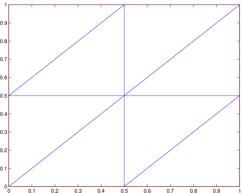
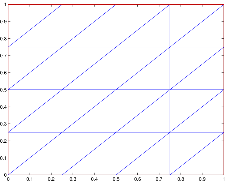
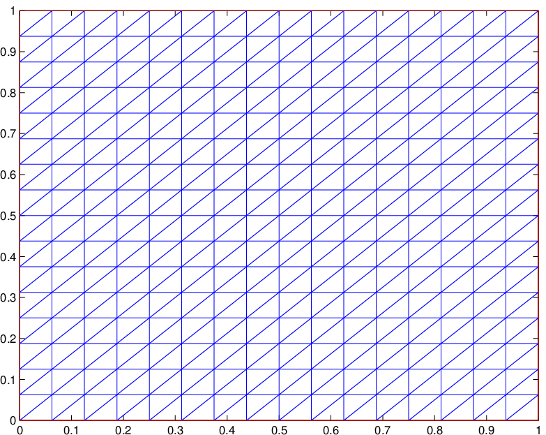
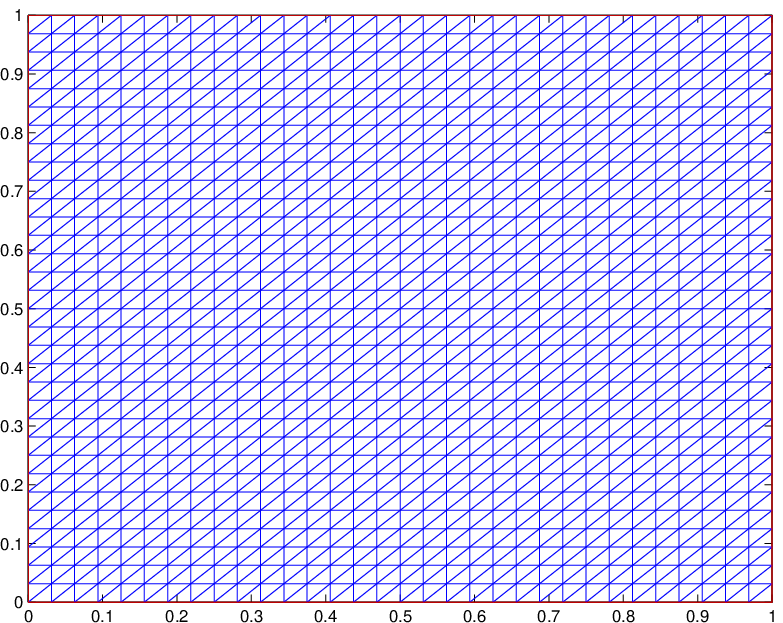
Here we report computed estimates of the condition number of our auxiliary-space preconditioned system matrix for the linear elasticity model discretized using various choices of mesh spacing on unit square . Here, represents the lengths of the horizontal and vertical sides of triangles in the meshes.
(a)
(b)
(c)
(d)
(e)
Figure 2. Meshes on the unit square
Experiment 1. We consider a pair of poisson equations on with homogeneous
Neumann boundaries:
(14)
We note that is the isomorphism associated with the weak formulation of (14) on
the space . The results in Table 1 implies that the condition number of the preconditioned system of is bounded independent of mesh size .
iter
20
24
27
27
27
1.92e+1
2.80e+1
3.51e+1
4.02e+1
4.39e+1
Table 1. Condition numbers .
Experiment 2. We deal with a special case when . Namely, the linear elasticity
reads
(15)
where represent four sides of the unit
square for . Also, without loss of generality, we suppose
that , here and later. Assume that
the body force is defined by
(16)
Then the exact solution is
We see that is the isomorphism associated with the weak formulation of (15) on .
In Table 2, , where and are the
smallest and largest constants satisfying:
iter
19
19
17
16
15
6.47e+0
6.70e+0
6.71e+0
6.67e+0
6.48e+0
Table 2. Condition numbers .
In Table 2, we observe that the preconditioner we devised is an efficient
preconditioner for the special case. Namely, .
Experiment 3. In this experiment, we study more general linear elasticity problems
with various :
(17)
where
and are defined as in Experiment 2. In Tables 3, 4
and 5, , where and are the
smallest and largest constants satisfying:
iter
iter
iter
24
1.33e+1
30
4.60e+1
33
8.60e+1
28
1.39e+1
39
4.51e+1
50
8.60e+1
25
1.40e+1
43
4.57e+1
55
8.55e+1
23
1.40e+1
40
4.56e+1
53
8.55e+1
21
1.39e+1
36
4.54e+1
46
8.49e+1
Table 3. Condition numbers .
Experiment 4. For small , we experiment the linear elasticity with homogeneous
pure traction boundary condition:
(18)
where are also defined as in Experiment 2 and the body force is such that
is the exact solution of (18). The results reported in Tables 4 indicate that the condition number of our preconditioned operator remains bounded independent of mesh size and, hence, provides for an optimal order preconditioner for our linear elasticity model problem. They coincide with our theoretical result that , independent of . We note that although our experiments have been carried out on a structured grid, our analysis carries over to unstructured simplicial meshes and our scheme is thus expected to perform similar for unstructured grids as well.
iter
norm
iter
norm
iter
norm
26
1.42e+1
7.71e-3
32
4.60e+1
1.10e-2
35
8.60e+1
1.25e-2
31
1.39e+1
4.07e-3
46
4.60e+1
7.56e-3
56
8.60e+1
9.62e-3
31
1.41e+1
1.41e-3
53
4.58e+1
3.48e-3
68
8.56e+1
5.21e-3
31
1.41e+1
3.91e-4
54
4.59e+1
1.12e-3
73
8.58e+1
1.92e-3
31
1.41e+1
1.01e-4
54
4.59e+1
3.04e-4
72
8.58e+1
5.49e-4
Table 4. Condition numbers and the discrete errors between the exact solution and the numerical solution.
Challenging experiment. It is well known that the performance of the
piecewise linear finite elements deteriorates as approaches . In the elasticity literature, it is called the locking phenomenon (see [5, 4] for more information). To overcome the effects of the locking, several methods have been suggested in [2, 6, 10, 9, 12, 14, 17]. Both our theoretical and numerical results show that the GFEM-based auxiliary preconditioner for the linear elasticity problem with small works very efficiently. It would also be worthwhile to investigate the numerical results when the preconditioner is applied to linear elasticity for large . We observe in Table 5 that
even when is large enough, the condition number of the preconditioned systems is bounded independent of mesh size and the discretization error estimates look reasonable if is sufficiently small.
iter
norm
iter
norm
iter
norm
iter
norm
92
4.06e+2
1.39e-2
109
8.06e+2
1.51e-2
134
4.01e+3
1.65e-2
140
8.01e+3
1.66e-2
114
4.06e+2
1.04e-2
144
8.06e+2
1.25e-2
224
4.01e+3
1.57e-2
258
8.01e+3
1.64e-2
135
4.06e+2
5.75e-3
170
8.06e+2
8.06e-3
287
4.01e+3
1.31e-2
365
8.01e+3
1.47e-2
145
4.05e+2
2.19e-3
183
8.06e+2
3.69e-3
322
4.01e+3
8.78e-3
404
8.01e+3
1.12e-2
143
4.05e+2
6.42e-4
192
8.05e+2
1.21e-3
367
4.00e+3
4.32e-3
455
8.01e+3
6.36e-3
Table 5. Condition numbers and the discrete errors between the exact solution and the numerical solution.
6. Concluding remarks
In this paper, using the auxiliary space technique we have designed a preconditioner for the solution of the problem of linear elasticity, which is also based on generalized finite element methods. We have proved that for arbitrarily fixed , the GFEM-based auxiliary preconditioner always works optimally for the system of linear elasticity discretized using the lowest finite element shape functions.
References
[1]
Douglas Arnold.
Lecture note on linear plate theory: modeling, analysis, and
computation.
[2]
Douglas N. Arnold, Franco Brezzi, Richard S. Falk, and L. Donatella Marini.
Locking-free Reissner-Mindlin elements without reduced
integration.
Comput. Methods Appl. Mech. Engrg., 196(37-40):3660–3671,
2007.
[3]
Douglas N. Arnold and Ragnar Winther.
Mixed finite elements for elasticity.
Numer. Math., 92(3):401–419, 2002.
[4]
Ivo Babuška and Manil Suri.
Locking effects in the finite element approximation of elasticity
problems.
Numer. Math., 62(4):439–463, 1992.
[5]
Ivo Babuška and Manil Suri.
On locking and robustness in the finite element method.
SIAM J. Numer. Anal., 29(5):1261–1293, 1992.
[6]
Susanne C. Brenner.
A nonconforming mixed multigrid method for the pure traction problem
in planar linear elasticity.
Math. Comp., 63(208):435–460, S1–S5, 1994.
[7]
Susanne C. Brenner and L. Ridgway Scott.
The mathematical theory of finite element methods, volume 15 of
Texts in Applied Mathematics.
Springer-Verlag, New York, 1994.
[8]
Susanne C. Brenner and Li-Yeng Sung.
Linear finite element methods for planar linear elasticity.
Math. Comp., 59(200):321–338, 1992.
[9]
Z. Cai, C.-O. Lee, T. A. Manteuffel, and S. F. McCormick.
First-order system least squares for linear elasticity: numerical
results.
SIAM J. Sci. Comput., 21(5):1706–1727 (electronic), 2000.
Iterative methods for solving systems of algebraic equations (Copper
Mountain, CO, 1998).
[10]
Zhiqiang Cai, Thomas A. Manteuffel, Stephen F. McCormick, and Seymour V.
Parter.
First-order system least squares (FOSLS) for planar linear
elasticity: pure traction problem.
SIAM J. Numer. Anal., 35(1):320–335 (electronic), 1998.
[11]
D. Cho and L. Zikatanov.
A multilevel preconditioning for generalized finite element method
problems on unstructured simplicial meshes.
J. Numer. Math., 15(3):163–180, 2007.
[12]
Richard S. Falk.
Nonconforming finite element methods for the equations of linear
elasticity.
Math. Comp., 57(196):529–550, 1991.
[13]
Leopoldo P. Franca and Rolf Stenberg.
Error analysis of Galerkin least squares methods for the elasticity
equations.
SIAM J. Numer. Anal., 28(6):1680–1697, 1991.
[14]
Chang-Ock Lee.
A conforming mixed finite element method for the pure traction
problem of linear elasticity.
Appl. Math. Comput., 93(1):11–29, 1998.
[15]
S.V. Nepomnyaschikh.
Decomposition and fictitious domains methods for elliptic boundary
value problems.
SIAM, Philadelphia, pages 581–613, 1992.
Fifth International Symposium on Domain Decomposition Methods for
Partial Differential Equations.
[16]
Yousef Saad.
Iterative methods for sparse linear systems.
Society for Industrial and Applied Mathematics, Philadelphia, PA,
second edition, 2003.
[17]
Joachim Schöberl.
Multigrid methods for a parameter dependent problem in primal
variables.
Numer. Math., 84(1):97–119, 1999.
[18]
J. Xu.
The auxiliary space method and optimal multigrid preconditioning
techniques for unstructured grids.
Computing, 56(3):215–235, 1996.
International GAMM-Workshop on Multi-level Methods (Meisdorf, 1994).
[19]
Jinchao Xu.
Iterative methods by space decomposition and subspace correction.
SIAM Rev., 34(4):581–613, 1992.