Path Integral for Stochastic Inflation: Non-Perturbative Volume Weighting, Complex Histories, Initial Conditions and the End of Inflation
Abstract
In this paper we present a path integral formulation of stochastic inflation, in which volume weighting can easily be implemented. With an in-depth study of inflation in a quartic potential, we investigate how the inflaton evolves and how inflation typically ends both with and without volume weighting. Perhaps unexpectedly, complex histories sometimes emerge with volume weighting. The reward for this excursion into the complex plane is an insight into how volume-weighted inflation both loses memory of initial conditions and ends via slow-roll. The slow-roll end of inflation mitigates certain “Youngness Paradox”-type criticisms of the volume-weighted paradigm. Thus it is perhaps time to rehabilitate proper time volume weighting as a viable measure for answering at least some interesting cosmological questions.
I Introduction
Inflation driven by the potential energy of some effective scalar field [1, 2, 3] has become a common explanation of the starting state of the radiation-dominated hot big bang model. A key reason for its acceptance is that small quantum fluctuations during the last 60 or so efolds of inflation can develop into almost scale invariant curvature perturbations [4, 5, 6] like those that we see today in the cosmic microwave background fluctuations [7]. Couplings in the inflaton’s potential have to be chosen to be very small in order to get the amplitude of the fluctuations suitably low. However, fluctuations in the scalar field increase as the background energy density increases, so in certain circumstances the fluctuations might have a significant effect on the evolution of large patches, leading to “stochastic inflation” [8]. Such fluctuations might lead to a situation in which part or even in some sense the majority of the universe continues to inflate for all time, i.e. “chaotic eternal inflation” [9].
The advent of the “string landscape” [10, 11] with its complicated vacuum structure has reinvigorated the search for a suitable measure on inflationary histories in situations where more than one possible history can be conceived of. Much of the debate revolves around the extent to which predictions should be conditioned on observations and, if more inflation leads to more observers, whether and how any “volume-weighting” should be implemented. For technical reasons much of this recent work has focussed on models where the inflaton is expected to “tunnel” from one vacuum state to another via bubble nucleation [12, 13, 14, 15, 16, 17, 18, 19, 20]. [21] is an exception, considering random initial conditions in random potentials, and the “reheating-volume” approach has been applied to both stochastic and bubble nucleation models [22, 23, 24]. Quantum cosmological studies [25, 26, 27, 28, 29, 30, 31, 32, 33, 34] provide complementary perspectives.
The approach discussed in this paper illuminates and expands the approach to stochastic inflation and volume-weighting presented in [35], in which one follows the evolution of the inflaton in a potential in proper time with a Langevin noise term approximating the quantum fluctuations. There expectation values were calculated for the field history and perturbatively corrected for the effects of volume weighting. By allowing for final-time constraints on the field value and considering weighting field values at some time by either the volume at that time or the volume at the final time, [35] began to directly attack the two issues in the debate mentioned above. The current paper addresses more general inflationary models than and in some sense corrects the perturbative conclusions of [35] via a non-perturbative treatment of volume weighting by way of a path integral. The change in viewpoint is similar to that in going from the Heisenberg approach to the Feynman approach in quantum mechanics when trying to address a question about the history of the system. An early approach to a Langevin model of stochastic inflation was presented by Hodges in [36]; more recent work includes [37, 38]. Refs. [39, 40] also address eternal inflation in a related manner. In contrast, much of the early work on stochastic eternal inflation [41, 42, 43, 44, 45] attempted to follow in time the evolution of a probability distribution for the inflaton with a Fokker-Planck equation (analogous to the Schrodinger approach to quantum mechanics). Such approaches typically broke down after a finite time, when the probability became unnormalizable rising rapidly with field value, leading to the suspicion that Planck-scale effects might be vital in controlling the theory and restoring predictivity. This led in part to proper time volume weighting falling out of favour as a measure on eternal inflation. In addition, puzzles such as the “Youngness Paradox” [46] (—if a fraction more inflation produces exponentially more volume, aren’t the most common observers at a given time the youngest ones conceivable?—) seem particularly acute with proper time volume weighting. We will see the surprising way in which a constrained path integral approach mitigates all these issues and so it may be suggested that proper time volume weighting should be reinstalled as a useful measure for at least some calculations in stochatic inflation.
This paper is organised as follows. First, a measure on slow-roll inflationary histories is presented. Saddle points of histories are discussed, and then volume-weighting is introduced. The model is studied in depth, and the way inflation typically ends is investigated. Finally there is a discussion and conclusions.
II A Measure on Slow-Roll Histories
In this section we derive a measure on slow-roll inflationary histories, starting from the appropriate Langevin equation for slow-roll inflation (see e.g. [35]; note that for comparison with other works a factor omitted there has been restored here):
| (1) |
where is a Gaussian-normalized white noise term and
| (2) |
with being the reduced Planck mass (henceforth assumed to be unity). One might think of Eq. (1) as describing the evolution of a member of an ensemble of physical-Hubble-volume sized regions forward in time. Note that (2) determines as a function of , and thus the scale factor at a time as a function of the history of up to time .
Now consider an arbitrary history . After a short time , the field will be at , a change of . From (1), the change of the field should be centered on with a variance of . So the probability of this segment of history occurring is:
| (3) |
Multiplying to obtain the joint probability for the entire history, and taking the limit , we obtain:
| (4) |
with a “Euclidean Lagrangian”
| (5) |
Furthermore, inspection of (3) suggests a change of variable that both renders the prefactor in (4) independent of field and makes the kinetic term in (5) canonical (up to a surface term):
| (6) |
leading to
| (7) |
up to a numerical factor. Here
| (8) |
with
| (9) |
expressed in terms of .11 1 An alternate derivation following the lines of [47] can yield a determinant correction to the measure coming from the change of variables from noise realizations to field realizations. For the variable for a potential, this determinant is independent of field so both derivations agree precisely. Given the already heuristic nature of our starting point, Eq. (1), we do not consider such corrections further in this work.
III The Path Integral and its Saddle Points
Given a general measure on histories along with a specification of the class of histories to integrate over, one may calculate the expectation value of some quantity of interest, say, with a path integral:
| (10) |
Note that can be of a very general nature, either local or non-local in time for example.
As in the Feynman path integral approach to quantum mechanics, it is often useful to look for saddle points in approximating (10). Corresponding to (7) for example we would take , and, certainly in this case, finding saddle points is very simple, since the lagrangian is equivalent to that for a point mass moving in some potential. There even exists a conserved energy. Furthermore, we can work with either or , the saddle points in either variable being equivalent.
Once we have the saddle point solution for given initial and final data, we can use it to approximate the probability density for that final data given the initial data by integrating (7) in a gaussian approximation. The leading term is simply the exponential of minus the action evaluated for the saddle point. By varying the field value at the final time and recalculating the saddle point solution and the (approximate) probability density, we can build up a picture of the probability distribution function at the final time. By repeating the procedure for different final times, we can build up a picture of the evolution of the probability distribution function in time. For (7), we thus find an approximate solution to the Fokker-Planck equation corresponding to (1).
We can also calculate the expectation value of in the saddle point approximation. For a fixed final field value, we just evaluate the quantity for the related saddle point solution. To relax the final field value constraint, we compute the average of calculated for all final field values, weighted by the exponential of minus the action (possibly multiplied by the gaussian prefactor for higher accuracy) for the corresponding final field value.
Let us quickly derive some useful results. Assuming the action is expressible as an integral over a local-in-time Lagrangian , then we can introduce a momentum
| (11) |
and Hamiltonian (primed to avoid confusion with the Hubble parameter ) and corresponding energy . Just as in classical mechanics (see e.g. [48]), evaluating the action as a function of end point and end time, we have . So, at a fixed final time , the action is extremized for a solution which both obeys the equations of motion and has . This, neglecting prefactor corrections, gives the extremum in the probability distribution function for at time .22 2 Note that here, unlike in most classical mechanics applications, one does have to be careful not to discard total integrals, which, while not altering the saddle point solution, affect the total value for the action and so the probability for a history. As long as does not involve , implies at time , i.e. a trajectory corresponding to an extremum in the probability distribution at time is slow-rolling as is approached. This does not necessarily imply that the trajectory slow-rolls all the way from to , nor that extrema of the probability distribution evolve according to slow-roll as is varied. However, in the simple case when is just , both of these statements do in fact hold. A helpful way to verify such statements is to look at the (conserved) energy associated with each saddle point solution. For , this is just
| (12) |
and for a solution that slow-rolls at the end time , we see . As is conserved along the saddle point, we see that must equal back along the entire trajectory to at , i.e. the saddle point is just the slow-roll solution evolved from the initial condition to the time . Hence as changes the position of the peak also follows the slow-roll solution in this case.
IV The Volume-Weighted Path Integral
Now we volume-weight. We do this by “reweighting” the measure from above by an appropriate term, and then renormalizing. We might imagine the physical-Hubble-volume sized regions followed above as being ‘‘probes’’ of much larger volumes of space that are inflating and so expanding in time. Thus the term is typically just the ‘‘final’’ volume33 3 One could also for example consider weighting by the volume at an intermediate time for calculating a final-field-value-constrained “rolling” volume average.
| (13) |
Because of the local-in-time nature of the exponent, we see that such volume weighting can be incorporated very simply by thinking of as an integral over of a more general “Euclidean Lagrangian”
| (14) |
We have only had to add a local-in-time term to the potential for . This extra term alters the constrained histories relative to the non-volume-weighted ones with the same boundary conditions.
The volume-weighting term, only involving the field and not its derivative, will not affect the expression for the momentum in terms of the field and its derivative. So, as for the non-volume-weighted case discussed above, the most probable trajectory will obey the slow-roll condition at the very end.
However, unlike before, this trajectory will not have slow-rolled all the way from the initial condition; there are two additional effects that cannot generally cancel. First, the equation of motion now has an extra field-dependent term. Second, the expression for the energy has an additional term, so, evaluating this at the end of the trajectory, the energy of the solution is moved from zero to . Thinking momentarily of as a function of at time for the most probable solution, we have
| (15) |
Changing and as discussed to incorporate volume-weighting will change and so considered as a function of : the peak of the probability distribution function does not now follow slow-roll.
We can now ask whether or not inflation ends in the rolling-volume-weighted average. If it does, the peak of the probability distribution function should pass through a field value corresponding to a small value of , i.e. the conserved energy should be able to have a small value. Evaluating the energy, expressed in terms of , at the initial condition thus leads to the condition:
| (16) |
for inflation to end in the volume-weighted average. Now, whatever the value of , if the potential term contribution to the left hand side is positive then inflation cannot end. So if
| (17) |
then inflation cannot end in the volume-weighted average (c.f.[39]). This precise constraint is consistent with the qualitative arguments of e.g. Guth [46] comparing the classical movement of the field to the quantum fluctuations in the field over a Hubble time. We may say that inflation is indeed “eternal” if the field starts at a value such that (17) is satisfied. Note that for this requires .
Let us assume that the field starts above the eternal inflation threshold and ask what happens. Does the volume-weighted field asymptote to some constant value, and if so can this value be above or below the starting value? Or does the field average run away to a place of infinite energy density, in either finite or infinite time? We are minded here of the early results looking at volume-weighted eternal inflation by solving the Fokker-Planck equation for say a potential; there it seemed that the probability distribution lost its extrema after a finite amount of time, becoming unnormalizably peaked at an infinite field value. This led to the imposition of arbitrary boundary conditions at the Planck density and the view that the volume-weighted field would quickly tend to its largest possible value and stay there inflating at the maximum possible rate. We indeed find, investigating as a specific example as discussed in the following section, that the average can stop existing after a finite time. Above we showed that the paths corresponding to extrema of the probability distribution must end in slow-roll. This applies to both maxima and minima, and a minimum in the probability distribution will delimit a formal unbounded rise in probability towards very high energy from a physical region of field values with its own maximum. As time goes on, the maximum and minimum merge; the probability distribution steadily increases with field energy. To see whether trajectories with Planckian energy densities are important or not for the disappearance of the average, we now though can look at the critical saddle point history and see whether or not it approaches the Planck density at any stage. For small coupling it turns out it does not and so we conclude that Planck scale effects will not affect the disappearance of volume-weighted average.
One may be concerned that the disappearance of the average is indicating a failure with the whole approach. However, we can continue to find constrained paths to lower field values, at least for a finite window of larger time intervals. So perhaps the correct interpretation is simply that answering the question “what is the field average on a surface of constant proper time?” is becoming problematical. But because we can still answer other questions, about constrained paths say, proper time volume weighting itself is not obviously failing at this stage.
Pushing to larger time intervals still, we find for at least that real histories connecting the inflationary initial conditions to low field values cease to exist. Surely even constrained proper time volume weighting is failing now? This is not necessarily the case because complex histories now emerge that link the initial and final conditions. Further, as we will see below, these complex paths are very close to being real towards the end of inflation, and indeed basically become “classical” slow-roll trajectories, insensitive to the initial field value or indeed the time interval between the initial and final conditions.
V in Depth: Complex Histories, Initial Conditions and the End of Inflation
For , is proportional to , which is in turn proportional to the Hubble radius which we denote here by and work with in order to allow for easy comparison with [35]. Introducing the (dimensionless) constants and , we find
| (18) |
Saddle-point histories satisfy
| (19) |
with a conserved energy
| (20) |
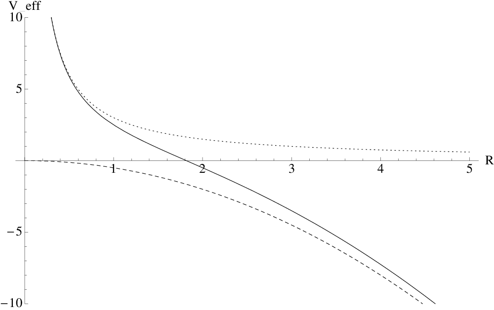
See Fig. 1 for the associated effective potential that the variable feels. (Note that in all plots and have been rescaled to absorb and via , .)
As discussed in Sec. IV, the momentum
| (21) |
has to be zero at the end of a history that finishes at an extremum of the probability distribution function at time . Hence, from (20), the energy of such a path is , which is small for weak coupling (of order ) if corresponds to for which inflation would classically be ending. Eternal inflation is inevitable if ever becomes less than (the zero of the effective potential in Fig. 1).
Fig. 1 is very helpful for understanding the nature of the (real) saddle point solutions, illustrating the discussion of Sec. IV. Let us look for solutions connecting to (“i” for initial, “f” for final). If , there are two classes of solutions differentiated by the sign of the initial velocity. One rolls up the potential, turns round and rolls back down past on the way to ; the other rolls straight down the potential from to . If , there are again two classes of solution, now differentiated by the sign of the final velocity. In one, rolls straight up the potential from to , in the other, rolls up the potential passing through , then rolls back down to . If , there is only one class of solution, rolling up the potential and then back down. In all cases, varying the initial speed, or equivalently the energy , changes the time needed to go from to .
Scanning over , and the velocity sign and recording the time each solution takes gives us complete information about the behaviour of the probability distribution function for as a function of . Note though that there is no guarantee that arbitrarily large values of will be obtained in the scan, and indeed turns out to be bounded when volume weighting is switched on.
If we temporarily focus on the subset of histories with zero final momentum (and so with energy with volume-weighting, or with without), corresponding to the extrema of the probability distribution function, we can build up a sketch of the loci of the maxima and minima of the probability distribution function as a function of time as in Fig. 2.

Without volume-weighting, a solution exists for any (the field spending longer and longer at small as increases), with always greater than , and the distribution moves (exponentially in time) to larger as time passes. Switching on volume weighting corresponds to adding a repulsive force, requiring to start with a more negative velocity than for the non-weighted case with the same and . Thus gets smaller more rapidly as expected; volume-weighting favours higher field values. Starting well below the eternal inflation threshold, the picture is qualitatively similar to the non-volume-weighted case. Starting above the eternal inflation threshold, the picture changes significantly however. The steep, “brick-wall”, nature of the repulse volume-weighting term in the effective potential means that there is in fact an upper limit on how much can be increased by increasing the initial speed of . After this time there are no extrema; the probability density increases monotonically towards small . We are able to conclude that at some intermediate time, at some , the peak of the probability distribution turns around; the inflaton begins to climb back up its potential in the volume-weighted average. The largest value of attained can be deduced by equating the effective potential at to the energy evaluated at the end.
Returning to the general case, it may seem strange that constrained saddle point solutions linking to fail to exist for too large of a time difference. As mentioned above, the paradox is resolved by realizing that there is no necessity for the saddle point histories to be real. Just as in contour integration, where one may deform real contours into the complex plane to pass through a saddle point in order to apply the method of steepest descents, we can do likewise here. Indeed, the use of complex histories has a precedent in the Euclidean “No-Bounday” approach to quantum cosmology, where for “large” final three-geometries the Euclidean path integral has a complex saddle point with a Lorentzian part [25]. We need only preserve our boundary conditions, namely that and that . We see straight away that the imaginary component of has to be zero at both ends, but that there is no such constraint on the imaginary component of at the ends. Decomposing (19) into real and imaginary parts, we can visualize as a point moving in a two-dimensional force field as heuristically plotted in Fig. 3.

We note the (unstable) zero-force locations specified by . By tuning the solution so that it approaches one of these points with near zero speed, it is possible for to “loiter” there for as long as is needed. Solutions with a long loitering period must have a complex energy very close to that of the effective potential evaluated at the loitering point in question. This complex energy determines solutions that asymptotically reach the loitering point in the future from or from the past from . Appropriate deviations in the initial velocities will “connect up” the two asymptotic solutions and make the total solution last for the desired finite time .
For solutions linking inflaton values corresponding to starting above the eternal-inflationary threshold to field values towards the end of conventional inflation, the appropriate loitering points are the ones with a positive real component and non-zero imaginary component of . These will provide a conjugate pair of histories. Each history will approach its respective loitering point and then roll back towards the real axis out to large positive values of .
Focusing on a single member of a conjugate pair for clarity, the way the solution reaches will become almost independent of how large is, as long as is sufficiently large. We thus see in a precise way how eternal inflation “loses memory” of initial conditions, in that, at sufficiently late times, the way inflation typically ends is very insensitive to the initial field value.
Note that for weak coupling the history need not go particularly close to and the Planckian energy densities there. Rather, the amplitude of the loitering points corresponds to , of order the eternal inflation threshold. Hence conclusions drawn from the history may hoped to be insensitive to any Planck-scale corrections to the model.
The imaginary part of a trajectory corresponding to the late-time end of eternal inflation for weak coupling is very small, and the real part of the field basically slow-rolls, as illustrated in Fig. 4.

These statements can be made quantitative by rearranging (20) to express in terms of and ,
| (22) |
the fractional correction over the slow-roll result () being small when the modulus of is well away from the eternal inflationary regime.
We have just seen that where stochastic eternal inflation ends, it basically ends classically. This might appear counter-intuitive, given the Youngness Paradox arguments about proper-time volume weighting. Consider looking for regions where the inflaton, if it slow-rolled, would have either one or two efolds say left to go. The Youngness Paradox would suggest that there are exponentially many more regions with one efold left than regions with two efolds left, the latter histories being “younger” and so having had more inflation in their past. One might have also thought that to the past of any of these regions the field would be much higher up its potential than slow-roll would suggest, perhaps even up at Planck-density values, since such histories would have exponentially more volume. Our result is not inconsistent with the first conclusion but suggests that volume-weighting does not sufficiently dominate over classical motion for the second conclusion to apply also. Thus standard calculations of inflationary density perturbations are probably safe even in eternal inflation as long as the coupling is weak.
VI Discussion and Conclusions
We can assemble what we have learned above into a somewhat cogent picture of volume-weighted stochastic eternal inflation. The field must start off above the eternal inflationary threshold, and then we soon see the volume-averaged field stop decreasing and turn around and begin increasing, indicating that volume effects are outweighing classical drift. From this we may hope that a late-time “steady state” situation will arise with late-time results dominating any averaging. After a finite proper time, the volume-averaged field ceases to exist; the system is dominated by strong fluctuations and a “global” picture breaks down. Nontheless, we may choose to focus on the observationally relevant but rare regions of the universe where inflation happens to end. Then we find that inflation ends in practically the same slow-roll manner on all proper time slices and hence some level of predictability is restored. The saddle point histories deviate into the complex plane rather than continue to values far above the eternal inflation threshold, indicating that the conventional view of the inflaton as jumping up and down on its potential in the eternal inflation regime might be too simplistic. Because when inflation does end it basically ends in slow-roll, conventional density perturbation calculations should still apply, preserving the successful predictions of conventional treatments of inflation.
The general techniques and insights of this paper should apply to many large-field models of inflation. It would be interesting to investigate potentials with multiple vacua. Indeed, for “Mexican-hat” type potentials, , one can analytically obtain an expression for in terms of and so obtain an explicit formula for the effective potential for . Thus one could investigate volume-weighting for small-field models of inflation where would might expect its effect to be less pronounced than for the large-field case studied here. (Note that an early work [49] discusses an approximate path integral treatment of the behaviour of the inflaton in a “new” inflationary potential.) Numerical investigation of the determinant prefactor would be helpful in getting an idea in how “classical” the histories really are. The author has checked numerically that there are no negative modes satisfying the relevant boundary conditions for a sample of representative (real) histories, as one would hope. It would also be possible to go beyond slow-roll, obtaining fourth-order equations for the saddle point histories, though the precise way in which the quantum fluctuations are modelled might need to be thought through more carefully.
As in quantum mechanics, we have seen that a path integral approach is particularly useful when asking time-dependent questions and looking for semi-classical histories. It has given us a technique for calculating in volume-weighted eternal inflation that is relevant for observations. We have been able to demonstrate how inflation typically ends normally even with volume-weighting in a manner insensitive to the precise initial conditions. By retreating from demanding a global picture of the universe at all times and rather adopting a more “top-down” observationally relevant approach [28, 29, 35] the path integral has allowed us to push much further than in the Fokker-Planck approach without having to worry about Planck density issues. We have also obtained a different result about the behaviour of the volume-weighted average than in the Langevin treatment of [35]. This is possibly because that work only perturbatively expanded around the classical solution, implicitly forcing one to consider only the subset of histories in which inflation has to end.
Finally, let us return to the question of proper-time volume weighting itself. Rather than any intrinsic flaw in the scheme, perhaps it was the gauge-dependence of the questions that proper time volume weighting encouraged one to ask that led to the weighting getting a bad reputation (a canonical example of such a gauge-dependent question being “which value of the inflaton is most likely at a given time?”). A question that we have addressed in this paper is “how does inflation end at a given proper time?”. Seeing that the answer only depends very weakly on what that time actually is, we have been able to obtain a satisfactory answer to the more general reasonable question “how does inflation end?” even using proper-time volume weighting. So for at least some physically relevant questions perhaps proper-time volume weighting is not so bad after all.
Acknowledgements.
We thank Anthony Aguirre, Tom Banks, Paolo Creminelli, Jaume Garriga, Alan Guth, Thomas Hertog, Antony Lewis, James Martin, Paul Steinhardt, Neil Turok and Toby Wiseman for helpful discussions. This research was supported in part by a minigrant from The Foundational Questions Institute (fqxi.org). I am supported by STFC.References
- [1] A. H. Guth, Phys. Rev. D23, 347 (1981).
- [2] A. D. Linde, Phys. Lett. B108, 389 (1982).
- [3] A. J. Albrecht and P. J. Steinhardt, Phys. Rev. Lett. 48, 1220 (1982).
- [4] S. W. Hawking, Phys. Lett. B115, 295 (1982).
- [5] A. H. Guth and S. Y. Pi, Phys. Rev. Lett. 49, 1110 (1982).
- [6] J. M. Bardeen, P. J. Steinhardt, and M. S. Turner, Phys. Rev. D28, 679 (1983).
- [7] N. Jarosik et al. (2010), eprint 1001.4744.
- [8] A. Vilenkin, Phys. Rev. D27, 2848 (1983).
- [9] A. D. Linde, Phys. Lett. B175, 395 (1986).
- [10] R. Bousso and J. Polchinski, JHEP 06, 006 (2000), eprint hep-th/0004134.
- [11] L. Susskind (2003), eprint hep-th/0302219.
- [12] J. Garriga, D. Schwartz-Perlov, A. Vilenkin, and S. Winitzki, JCAP 0601, 017 (2006), eprint hep-th/0509184.
- [13] R. Easther, E. A. Lim, and M. R. Martin, JCAP 0603, 016 (2006), eprint astro-ph/0511233.
- [14] V. Vanchurin and A. Vilenkin, Phys. Rev. D74, 043520 (2006), eprint hep-th/0605015.
- [15] R. Bousso, Phys. Rev. Lett. 97, 191302 (2006), eprint hep-th/0605263.
- [16] A. Aguirre, S. Gratton, and M. C. Johnson, Phys. Rev. D75, 123501 (2007a), eprint hep-th/0611221.
- [17] A. Aguirre, S. Gratton, and M. C. Johnson, Phys. Rev. Lett. 98, 131301 (2007b), eprint hep-th/0612195.
- [18] A. D. Linde, JCAP 0706, 017 (2007), eprint 0705.1160.
- [19] A. De Simone et al. (2008), eprint 0808.3778.
- [20] A. D. Linde, V. Vanchurin, and S. Winitzki, JCAP 0901, 031 (2009), eprint 0812.0005.
- [21] M. Tegmark, JCAP 0504, 001 (2005), eprint astro-ph/0410281.
- [22] S. Winitzki, Phys. Rev. D78, 043501 (2008a), eprint 0803.1300.
- [23] S. Winitzki, Phys. Rev. D78, 063517 (2008b), eprint 0805.3940.
- [24] S. Winitzki, Phys. Rev. D78, 123518 (2008c), eprint 0810.1517.
- [25] J. B. Hartle and S. W. Hawking, Phys. Rev. D28, 2960 (1983).
- [26] S. W. Hawking and N. Turok, Phys. Lett. B425, 25 (1998), eprint hep-th/9802030.
- [27] S. Gratton and N. Turok, Phys. Rev. D63, 123514 (2001), eprint hep-th/0008235.
- [28] S. W. Hawking and T. Hertog, Phys. Rev. D66, 123509 (2002), eprint hep-th/0204212.
- [29] S. W. Hawking (2003), eprint astro-ph/0305562.
- [30] S. W. Hawking (2007), eprint 0710.2029.
- [31] J. B. Hartle, S. W. Hawking, and T. Hertog, Phys. Rev. Lett. 100, 201301 (2008a), eprint 0711.4630.
- [32] J. B. Hartle, S. W. Hawking, and T. Hertog, Phys. Rev. D77, 123537 (2008b), eprint 0803.1663.
- [33] J. Hartle and T. Hertog, Phys. Rev. D80, 063531 (2009), eprint 0905.3877.
- [34] J. Hartle, S. W. Hawking, and T. Hertog (2010), eprint 1001.0262.
- [35] S. Gratton and N. Turok, Phys. Rev. D72, 043507 (2005), eprint hep-th/0503063.
- [36] H. M. Hodges, Phys. Rev. D39, 3568 (1989).
- [37] J. Martin and M. Musso, Phys. Rev. D73, 043516 (2006a), eprint hep-th/0511214.
- [38] J. Martin and M. Musso, Phys. Rev. D73, 043517 (2006b), eprint hep-th/0511292.
- [39] P. Creminelli, S. Dubovsky, A. Nicolis, L. Senatore, and M. Zaldarriaga, JHEP 09, 036 (2008), eprint 0802.1067.
- [40] S. Dubovsky, L. Senatore, and G. Villadoro, JHEP 04, 118 (2009), eprint 0812.2246.
- [41] A. S. Goncharov, A. D. Linde, and V. F. Mukhanov, Int. J. Mod. Phys. A2, 561 (1987).
- [42] K.-i. Nakao, Y. Nambu, and M. Sasaki, Prog. Theor. Phys. 80, 1041 (1988).
- [43] M. Sasaki, Y. Nambu, and K.-i. Nakao, Phys. Lett. B209, 197 (1988a).
- [44] M. Sasaki, Y. Nambu, and K.-i. Nakao, Nucl. Phys. B308, 868 (1988b).
- [45] A. D. Linde, D. A. Linde, and A. Mezhlumian, Phys. Rev. D49, 1783 (1994), eprint gr-qc/9306035.
- [46] A. H. Guth, J. Phys. A40, 6811 (2007), eprint hep-th/0702178.
- [47] G. Parisi and N. Sourlas, Phys. Rev. Lett. 43, 744 (1979).
- [48] D. Park, Classical Dynamics and Its Quantum Analogues, Second Edition (Springer-Verlag, 1990).
- [49] S.-J. Rey, Nucl. Phys. B284, 706 (1987).