Chapter 1 LHC Detectors and Early Physics
Günther Dissertori
ETH Zurich, Switzerland
1 Introduction
At the time of writing these proceedings11 1 Lecture given at the 65th Scottish Universities Summer School in Physics: LHC Physics (16 August to 29 August 2009), St. Andrews (January 2010), we have just witnessed the successful re-start (after the sudden stop of operations in September 2008) of the world’s most powerful particle accelerator ever built. CERN’s Large Hadron Collider (LHC) has provided first collisions at injection energy (450 GeV per beam) and at the world’s record energy of 1.18 TeV/beam. Next it is expected that the centre-of-mass energy will be raised to 7 TeV during the year 2010.
Thanks to the unprecedented energies and luminosities, it will give particle physicists the possibility to explore the TeV energy range for the first time and hopefully discover new phenomena, which go beyond the so successful Standard Model (SM). Among the most prominent new physics scenarios are the appearance of one (or several) Higgs bosons, of supersymmetric particles and of signatures for the existence of extra spatial dimensions.
In this review I will try to sketch the basic criteria and boundary conditions which have guided the design of the LHC detectors. The discussion will concentrate on the so-called general-purpose experiments, ATLAS and CMS. After an overview of the detector’s characteristics and performance, I will elaborate on the expected measurements of hard processes, with emphasis on jet and vector boson production, i.e., tests of Quantum Chromodynamics (QCD) and Electroweak Physics.
There exist many excellent reviews on the topics which are addressed here. Without making an attempt to be comprehensive, I would like to mention the various articles which can be found in a recent book edited by Kane and Pierce [1]. Extensive material has been compiled by the ATLAS and CMS collaborations in their Technical Design Reports on the Physics performance [2, 3], and detailed descriptions of the detectors are given in [4, 5]. Finally, an excellent overview of the detector’s performance and their comparison can be found in [6].
2 Design Criteria for the Detectors
When designing large, general-purpose detector systems such as ATLAS and CMS, which have to operate in collider mode at an accelerator such as the LHC, obviously many aspects, constraints, boundary conditions etc. have to be taken into account. First of all, the expected Physics and the accelerator’s parameters drive the design in a significant way. The overall layout of the experiment is strongly determined by the choice of the magnet system(s). Finally, the tracking, calorimeter, muon and data-acquisition systems are built with the goal of optimal performance under the imposed boundary conditions and with the available technologies. In the following I will address these aspects and show how they have led to the experiments as they are built today. Here the aim is not to go into the very detail of the (technical) choices of ATLAS and CMS, but rather to discuss, also via some simple calculations, the basic parameters and their role in the development of the detectors.
Before entering the discussion, it is necessary to define the most relevant and often used kinematic variables and relations. The transverse momentum is defined as the component of a particle’s (or jet’s) momentum perpendicular to the beam line, i.e., , where and is the angle w.r.t. the beam line. When talking about energy () deposits in calorimeters (or jets built out of them), the transverse energy is introduced, . If the energy deposits are defined as vectors (by using their directions w.r.t. the interaction point), their negative vector sum gives the Missing Transverse Energy (MET, ). At hadron colliders the rapidity turns out to be a well-suited kinematic variable, because differences in rapidity are invariant under boosts along the beam direction. Here denotes the momentum component along the beam line. For massless particles the rapidity is equal to the pseudo-rapidity 22 2 Thus, polar angles of correspond to .. Indeed, the detector elements at hadron colliders are typically segmented in (pseudo-)rapidity intervals. Finally, the azimuthal angle around the beam direction is usually denoted as or .
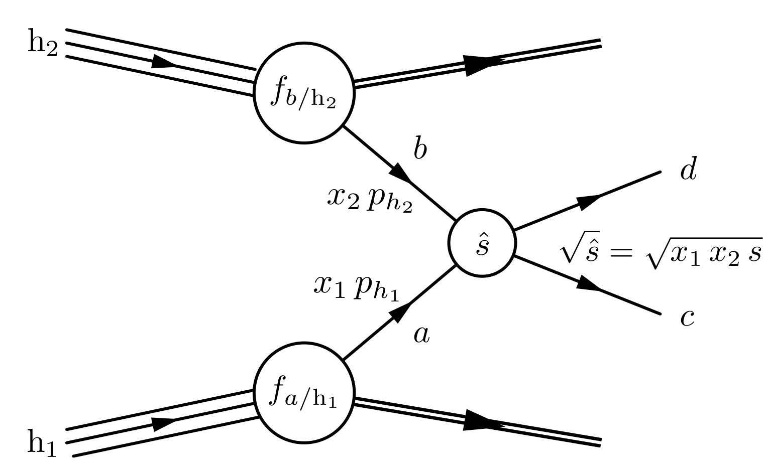
With these definitions at hand, we can now look at the basic kinematic relations relevant for the discussion of inelastic proton–proton scattering. Figure 1 shows the basic Feynman diagram for the description of inelastic hadron–hadron scattering. Two partons (quarks or gluons), which carry a fraction of the incoming hadron’s momenta , interact at a momentum transfer (or invariant mass) scale of , where is the squared centre-of-mass energy of the incoming hadrons. In the case of a heavy particle (or resonance) of mass being produced in the interaction of the two partons, we need . The energy and longitudinal momentum of the newly produced state are given by and (we neglect parton masses). By inserting this into the definition for the rapidity we obtain the relations
| (1) |
where is the rapidity of the particle with mass . If is very large (of the order of the total centre-of-mass energy), both momentum fractions have to be very large (and not too dissimilar), leading to , i.e., such states are produced at so-called central rapidity (). On the other hand, if the momentum fractions are very different, e.g. one of them is much smaller than the other, then the produced final state will have a strong boost and appear at large (positive or negative) rapidities. As a consequence, the decay products of heavy states (or particles from reactions at very large momentum transfer) will tend to appear at smaller rapidities (and thus “more centrally”, i.e., at larger polar angles) than those from the bulk of softer interactions.
2.1 Expected Physics
The main aspects of the Physics to be expected can be understood by studying figure 2. There we find the cross sections for various processes as a function of the proton–proton centre-of-mass energy. The total inelastic cross section, of the order of 60 - 70 mb, is completely dominated by soft collisions at low momentum transfer. Typically this bulk of interactions is called minimum bias events, since they will be registered with a minimal set of trigger conditions. Obviously, since these are the processes with the highest cross section (probability), they will show up first and require only a minimal selection. Depending on the exact geometrical acceptance and the detailed definition of these minimal trigger settings, also single- and double-diffractive events will contribute here, whereas the measurement of purely elastic proton–proton scattering relies on dedicated detectors in the far-forward part of the interaction region. It is worth noting that also hard-scattering events at large momentum transfer will pass the minimum bias trigger, and thus, in principle, are part of the minimum bias event sample. However, since their rate is so much smaller, the sample is basically populated by relatively soft collisions.
The average transverse momentum of charged particles produced in minimum bias events at 14 TeV centre-of-mass energy will be around 600 MeV and the most likely transverse momentum in the 200-300 MeV range (the exact values strongly depend on the model parameters, which are not well known so far, or on the extrapolations of fits to lower-energy data). From pure phase-space considerations, , we expect a basically flat distribution of charged particles in rapidity, up to the kinematic boundaries of around 5 units in rapidity where there is a sharp drop. Whereas earlier measurements (as well as the very first LHC measurements at 900 and 2360 GeV centre-of-mass energy [8, 9]) give slightly more than three charged particles per unit rapidity for the central plateau, at the higher LHC energies we expect up to six charged and 2–3 neutral particles per unit rapidity, uniformly distributed in . These numbers allow us to make the following conclusions:
-
roughly integrating the charged particle densities over the whole acceptance, we obtain particles per minimum bias event, for a maximum rapidity coverage of , and a total transverse momentum of GeV. If several minimum bias events occur at the same beam crossing, these numbers have to be multiplied accordingly. Thus it is important to have detectors with excellent coverage (hermeticity) up to rapidities of around 5, in order to collect the largest fraction of these particles and thus to avoid spurious measurements of ;
-
it will be important to actually measure these numbers and their energy dependence as quickly as possible, in order to tune the Monte Carlo predictions, which later will be used to model the contributions of such soft events to the energy flow in overlapping soft and hard-scattering proton–proton collisions;
-
in a strong solenoidal magnetic field, many of these soft charged particles will become curling tracks (“loopers”). If we would like to avoid too many of the soft particles to reach the calorimeters, thus reducing the occupancy there, we can use the simple equation to derive a minimal radius m of a cylindrical tracking detector inside a calorimeter system. Here denotes the bending radius of charged particles in a magnetic field . We have used GeV and T. Stronger fields and/or larger tracking systems will keep the calorimeters cleaner from these soft-event contributions, but induce more loopers, thus higher occupancy and more difficult pattern/track recognition in the tracker.
The next most-likely events to appear will be collisions containing two or more jets. Depending on the minimal threshold in , applied for triggering on such jets, the cross sections can grow up to hundreds of b. More interestingly, even the cross section for the production of jets above several hundreds of GeV are in the tens-of-nb range and thus much larger than at the Tevatron. Therefore LHC will quickly extend the jet range into uncharted territory and become sensitive to high-mass di-jet resonances, new contact interactions and/or quark compositeness. However, achieving such Physics goals quickly will require an excellent understanding of jet reconstruction. This vast topic includes the usage of modern jet algorithms (for a recent overview we refer to [10]), the data-driven determination of the jet energy scale, the combination of calorimeter and tracker information for obtaining an optimal jet energy scale and resolution, the understanding of pile-up energy and underlying event contributions, etc. The resulting detector requirements are an excellent (granular) calorimeter system up to large rapidities, combined with a high-performance tracking detector if the overall (charged and neutral) particle-flow reconstruction is used as input to the jet finding.
Once the integrated luminosities allow to be sensitive to processes with cross sections in the nb range, we start to explore the domain of electro-weak physics, starting with the production of bosons (plus anything), followed by and then top-pair production. The latter is up to 100 times larger than at the Tevatron, which justifies calling the LHC a top-factory. Since the cross sections for QCD jet production are many orders of magnitude larger than for these electro-weak processes, it is obviously hopeless to look for and decays into jets. Vector boson production is rather triggered on by their leptonic decays. This explains why a major effort went into the design of detectors with excellent lepton (electron, muon, tau) reconstruction capabilities. Further arguments for this can be found by looking at a list of benchmark processes, which were identified in the early days of the LHC planning to be well-suited for the study of electro-weak symmetry breaking, namely , , , , (Vector Boson Fusion, VBF), as well as new Physics such as . All these processes have cross sections (times branching ratios) of order fb, which immediately determines the necessary integrated luminosities for obtaining sensitivity to them. Again, this requires excellent lepton, photon and jet reconstruction. Since here the leptons (photons) are produced in decays of heavy objects, they will be triggered on by their relatively large transverse momentum (typically above GeV). Furthermore, as we have seen above, they tend to be produced at central rapidities, thus the relevant sub-detectors, such as the electromagnetic calorimeter or the muon system, have to be optimized for and cover only a restricted (pseudo)-rapidity range, typically up to . Altogether the above considerations lead us to the following additional detector requirements :
-
the detectors must be capable of triggering on and identifying extremely rare events, with cross sections some times the total cross section. This requires an online rejection of . Nevertheless, the overall event rates are very large and impose strong requirements on data handling and storage, with a yearly yield of events of a few MByte each;
-
leptons and photons should be well triggered on and measured with high resolution. This determines the performance of the electromagnetic calorimetry and the muon systems. In particular, an efficient electron reconstruction together with a jet fake rate33 3 This is the probability that a jet is mis-identified as an electron by the reconstruction algorithms. of about has to be achieved, in order to cope with the enormous jet background. Furthermore, an excellent energy resolution of the electromagnetic calorimeter will ease the identification of resonances over a very large background, such as ;
-
many of the electro-weak processes, such as top production, as well as new physics scenarios such as supersymmetric Higgs decays, involve the production of b-quarks and taus. This asks for silicon strip and pixel detectors, which give efficient b-tagging and tau identification. Here, jet rejection factors of at least are needed, for a b-tagging efficiency of .
2.2 The LHC Parameters
Evidently, the LHC machine parameters play a fundamental role in the design of the experiments. The ultimate centre-of-mass energy of 14 TeV will be reached in several steps, currently the most likely scenario is TeV. The maximal energy is basically fixed by the radius of the LEP tunnel and the available superconducting magnet technologies. During the early planning phases it became a clear design goal that the lower energy compared to the SSC in the US (20 TeV/beam) had to be compensated by a much higher luminosity. Previously we have seen that processes related to the electro-weak symmetry breaking have cross sections of order fb. If we assume a canonical running time per year of sec, we will need an instantaneous luminosity of cm-1sec fb-1sec-1 in order to accumulate events per year for a process with cross section fb. Luminosities in this range can only be achieved by large bunch intensities ( protons/bunch), a large number of bunches or equivalently a small bunch spacing ( ns) and a small beam size at the interaction regions (m). It is worth noting that a simple multiplication of instantaneous peak luminosity and running time gives a too optimistic estimate for the integrated luminosity. Decreasing luminosities during a fill, the time needed for the filling and acceleration cycles, machine commissioning and development, as well as other down-time periods can be accounted for by a heuristic efficiency factor of roughly .
At such high luminosities of cm-1sec, due to the very large total cross section, we expect the enormous rate of inelastic events of about events / sec. This allows us to calculate the number of inelastic events per bunch crossing, namely events, which will pile-up on top of a possibly interesting high- scattering event. These pile-up events will be soft proton–proton interactions, simply because it is the most likely thing to happen. Previously we have estimated that about particles are produced in such a soft collision, with a total of order GeV. Multiplying this by the number of pile-up events, we therefore expect more than particles carrying a total of more than TeV per bunch crossing. Good coverage and hermeticity become an even stronger requirement. At the same time, it is clear that dealing with these pile-up events in the detectors (and individual detector channels), as well as with the induced radiation levels, will lead to strong boundary conditions for the experiment’s design. Indeed, at the LHC design luminosity we expect ionising doses of Gy / /year, where is the transverse distance (in cm) to the beam. Damage can also be caused by photons created in electromagnetic showers and by the very high neutron fluences, in particular in the forward regions (up to n/cm2 over 10 years of LHC running).
The high bunch-crossing frequency, combined with the large-sized detectors, imposes a further technical challenge, related to the timing of the trigger and readout. Interactions occur every 25 ns. During such an interval, the produced particles travel a distance of roughly 7.5 m. This is to be compared to a typical LHC detector radius exceeding 10 m, and overall half-length beyond 20 m. Thus, the particles created in one or two previous crossings have not yet left the detector when the next ones are produced at the interaction point. Furthermore, one has to consider that the electronic signals from the detectors travel some 5 m during a 25 ns interval, and typical cable lengths are of order 100 m.
Altogether, these challenging conditions ask for highly granular and radiation-hard detectors, combined with fast readout (20-50 ns response time). High granularity helps to minimize pile-up effects in a single detector element. However, detectors with many channels (e.g. about 100 million pixels, 200 000 cells in an electromagnetic calorimeter) represent a strong cost factor.
2.3 The Choice of the Magnet System
The layout of the magnet system is among the most important of all design choices, since it fixes many other parameters of the experiment. Therefore it also has to come very early on in the development. Of course, the main purpose of the magnetic field(s) is to bend charged particles and thus to determine their momentum and their charge sign. Furthermore, strong fields help to keep most of the soft particles (cf. section 2.1) within cylindrical regions of small radius (see figure 3, right), thus reducing the occupancy and pile-up effects in the calorimeters. Concerning the momentum measurement, let’s recall the most relevant formulas. Typically the momentum of a charged particle track is not determined directly from the bending radius, but from the sagitta of a track’s segment within a detector region of length (see figure 3, left). Within the approximation we find . Then the momentum and its relative uncertainty are given by
| (2) |
where is the magnetic field strength (expressed in Tesla). We see that the measurement error can be minimized by maximizing the product , i.e., it is best to have large tracking systems (large lever arm) and strong fields. Obviously, both parameters will drive the overall cost of the experiment, in particular . It is also worth noting that the total bending power is proportional to , where is the particle’s path perpendicular to the magnetic field. With these basic relations in hand, we can discuss the choices made by ATLAS and CMS (figure 3, right). A detailed comparison and technical parameters can be found, e.g., in table 3 of Ref. [6].
 |
 |
CMS has opted for a single magnet system based on a large, high-field superconducting solenoid and an instrumented iron return yoke. This has led to a simple and compact overall design (determining by the way also part of the experiment’s name), giving excellent momentum resolution when combined with a powerful inner tracking system. The radius of the solenoid was its main cost driver, and m turned out to be affordable and technically doable. A magnetic field of T was realizable, whereas T would still deliver good physics performance. The current operating field of CMS is T. A single solenoid has the disadvantage of limiting the momentum resolution in the forward direction, at large rapidities (remember ), and choosing a large winding radius implies making the solenoid also very long in order to cover the largest possible rapidity. The instrumented return yoke (iron) limits the momentum resolution at low because of multiple scattering. This also impacts the trigger rates and the choice of the lower trigger thresholds. This is because the steeply falling momentum distributions, folded with a bad resolution, lead to a large feedthrough of soft particles beyond the trigger thresholds and thus to saturation. This is of particular concern for the stand-alone muon triggering at the foreseen large Super-LHC (SLHC) rates, since the multiple scattering effect cannot be overcome by installing additional and/or more precise muon tracking stations. A further important choice was to make the solenoid radius large enough in order to place the complete calorimetry (both electromagnetic and hadronic) inside the coil. Whereas this has the advantage of minimizing the amount of dead material in front of the calorimeter and therefore not compromising its intrinsic resolution, it implies that less than 2 m of radial extension are left for placing all absorbers, active calorimeter materials and readout, given that the tracker has a radius somewhat larger than 1 m. The implications are discussed in section 2.5.
ATLAS is characterized by a two-magnet system, with a solenoid (smaller radius than in CMS) in the inner part and a large air-core toroid surrounding the calorimeters. In view of an optimal performance with muons, a toroid has the advantage of very large and good bending power also in the forward direction. The problems related to multiple scattering and its impact on muon stand-alone triggering in a high-rate environment, as discussed above, can be minimized by an air-core toroid, which has no return yoke. It also keeps the calorimeters free of field and leaves large enough space for them. However, it determines the extremely large overall size of ATLAS and leads to a rather complex structure and complex magnetic field configurations. The latter is of particular concern in view of precise particle tracking, which needs excellent knowledge of the field map. Many coils would give a more uniform field, but obviously drive the cost very much. Indeed, the original proposal of 12 coils had to be reduced to 8 coils because of this. Furthermore, the large magnet structures ask for very large muon chambers, which then have to be aligned at precisions up to m, a formidable task. Because of the closed field lines around the calorimeters, a toroidal system has to be complemented by a solenoid which provides a field for inner tracking close to the interaction point. Since this solenoid is placed in front of the liquid-argon electromagnetic calorimeter, a lot of design work went into optimizing the materials and integrating the vacuum vessel for the coil with the cryostat for the barrel liquid-argon calorimeter, in order to minimize the dead material in front of the electromagnetic calorimeter. Also, the ATLAS solenoid is shorter than the one in CMS, which impacts somewhat the inner tracking performance at large rapidities because of the reduced field uniformity.
2.4 Tracking and Muon Systems
The basic requirements of a tracking system are:
-
allow for a robust and redundant pattern recognition, which is necessary for an efficient and precise reconstruction of all charged particles with momentum above GeV, up to pseudo-rapidities of ;
-
provide high-level triggering capabilities for electrons, taus and b-jets;
-
allow for an efficient and precise reconstruction of secondary vertices and impact parameters, which is of paramount importance for final states involving heavy flavours, in particular b-quarks;
-
complement and improve the electron reconstruction and triggering performance of the electromagnetic calorimeter by matching isolated tracks to calorimeter clusters;
-
provide some particle identification power, such as electron/pion separation, by a measurement of the specific ionization () or some other techniques, such as transition radiation.
When designing a tracking system, we have to deal with a fundamental problem of “conflicting interests”: many tracking layers will provide many hits for a robust track reconstruction. However, many channels will also require a large number of supports (cables, cooling, support structures etc.), which leads to a considerable amount of (dead) material in front of the calorimeters. This obviously jeopardizes the intrinsic resolution of the electromagnetic calorimeter, leads to a large fraction of photon conversions inside the tracker before reaching the calorimeter and causes multiple scattering of low-momentum particles. Indeed, the issue of the so-called material budget of the tracking systems has led to an “unfortunate similarity” between ATLAS and CMS, since in both cases the total material has increased by a factor of from their approval in 1994 to now. The material distributions reach peak levels of radiation lengths at rapidities around 1.5 (the transition region between barrel and endcap tracking stations is a preferred cable and support routing area). The consequences are that electrons lose between 25 and 70% of their energy by bremsstrahlung and that 20 to 60% of the photons convert into pairs before reaching the electromagnetic calorimeter. There exist algorithms for the recovery of energy loss by bremsstrahlung and for finding conversions, but obviously the overall reconstruction of electrons and photons is hampered by this.
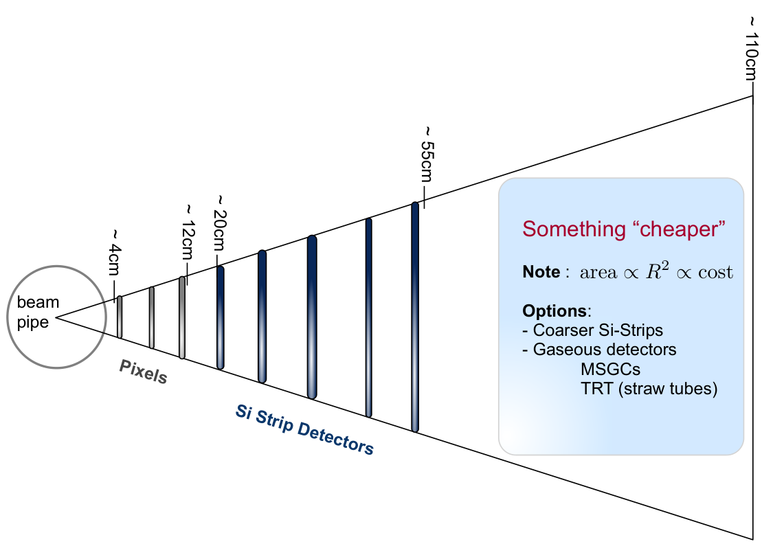
Concerning the intrinsic resolution requirements of the tracking detectors, we can look again at equation (2) and plug in some typical numbers, such as m and T. If we aim for a relative momentum resolution of 1% at GeV, we have to measure the sagitta with a precision of m. Therefore the individual hit reconstruction precision should be in this ballpark and definitely not much worse than m. Pattern recognition, impact parameter resolution and the large soft-particle flux at small (cf. section 2.2) ask for the smallest cell sizes and possibly three-dimensional hit reconstruction at the smallest radii. This optimizes the single-hit resolution and minimizes the occupancy and thus fake hit assignment. When going to larger radii, the requirements become less stringent, since the particle flux falls like and multiple scattering in the inner layers puts a natural limit on the achievable momentum resolution and thus on the necessary cell size (or pitch). On the other hand, the detector area grows with , and with it the number of channels and ultimately the costs. A careful optimization of all these ingredients has led the two collaborations to go for tracker designs with a basic structure as depicted in figure 4. Extremely high-performance pixel and silicon strip detectors in the innermost regions, with unprecedented numbers of channels and overall areas, are complemented with a straw-tube tracker (ATLAS) or a larger-pitch silicon strip system (CMS) at larger radii. The straw-tube tracker gives a very large number of hits and in addition, via transition radiation layers, also provides an electron/pion separation. For the all-silicon choice of CMS it is worth noting that the outermost tracking layer has a similarly fine pitch like a few layers at intermediate radii. This provides better accuracy at the end of the lever arm than in ATLAS, hence a more than a factor of 2 better momentum resolution at . The CMS pixel detector is engineered in a manner which allows quick and easy installation and removal, a non-negligible feature in view of many years of LHC running and the necessary shut-down periods in between. A comparison of the final tracking systems of ATLAS and CMS can be found in tables 4 and 6, and of their performance in table 7 of Ref. [6]. In terms of momentum resolution the CMS tracker turns out to be superior to that of ATLAS ( at GeV and central rapidity, compared to ), in particular at larger rapidities. This is because of the stronger magnetic field and its better uniformity over the whole tracker region. On the other hand, the vertexing and b-tagging performances are similar, and the impact of the material and the larger -field seem to be visible in slightly lower reconstruction efficiencies (80-85%) for low-momentum pions and electrons in CMS, compared to ATLAS (84-90%).
The tracking systems described above play an important role also for the momentum measurements of muons. However, when designing the muon systems, further requirements have to be taken into consideration:
-
muon momenta up to 1 TeV should be reconstructed at a precision of 10%, over a wide rapidity range;
-
the mass of high-mass di-muon resonances, such as a hypothetical with mass of , should be reconstructed at a precision of 1%;
-
muon identification has to be performed in a very dense environment, and if needed the systems should be capable of triggering on and measuring muons above GeV in stand-alone mode;
-
muon identification and triggering should be based on robustness and redundancy, with radiation-hard detectors and various readout speeds. This can be achieved by combining different technologies for the muon chambers.
The issue of stand-alone muon reconstruction has already been addressed above. Whereas the interaction point as additional constraint helps to achieve this in CMS, the multiple scattering poses some limitations, which are avoided by air-core toroids in ATLAS. The effect of multiple scattering on the momentum resolution can be modeled by
| (3) |
If we choose for the particle’s velocity, T, m and a radiation length of m, as is the case in the iron return yoke of CMS, we find a relative uncertainty of , which places an absolute limit on the achievable resolution. Further issues are the unprecedented challenges to be faced by the alignment systems and the punch-through of pions from the calorimeters.
The ATLAS muon spectrometer excels by its stand-alone reconstruction and triggering capabilities and its large coverage () in open geometry. At the same time, the complicated geometry and field configurations lead to large fluctuations in acceptance and performance over the full potential area. The CMS muon system allows for a superior momentum resolution in the central detector regions, when combining the information from the inner tracker with the muon chambers. This overall excellent resolution is degraded in the forward regions (), where the solenoid bending power becomes insufficient. In addition, the limitations on stand-alone triggering under high-rate conditions have already been discussed. Again, a detailed comparison of the systems can be found in [6] (tables 11 and 12), and their basic layouts are depicted in figure 5.
 |
 |
2.5 Calorimetry
Calorimeters play a central role in the reconstruction and (transverse) energy measurement of electrons, photons and hadronic jets. Whereas the best energy/momentum resolution for low- and medium- particles is obtained with spectrometers, at very high the calorimeters take over, as can be seen from
| (4) |
This is also one of the reasons why calorimeters provide essential information for triggering on high- objects. At LHC they have to absorb particles and jets with energies up to the TeV region. This has the following implications: The position of the maximum of a shower, which develops in a calorimeter, grows like , namely , where and are the radiation length and critical energy of an absorber material (see, e.g. [12]). In order to well contain an electromagnetic shower of order 1 TeV we need an absorber thickness of , similarly, for containing a hadronic jet of 1 TeV we need roughly . Here is the effective interaction length of the system. Now let’s take some concrete examples, such as Lead-Tungstate (PbWO4) for the electromagnetic calorimeter (ECAL). We have cm, which implies that for this ECAL, leaving also some space for the readout electronics, we have to foresee at least some 50-60 cm of radial space. On the other hand, if we choose iron as absorber material for the hadronic calorimeter (HCAL), we find cm and thus require about 180 cm of radial thickness in order to fully contain 1 TeV jets. However, if we remember the constraints in the CMS design, mostly given by the coil diameter and the tracker size, we observe that m (cf. figure 6). Thus, instead of 11 interaction lengths there is only space for 6, or when counting also the ECAL material in front of HCAL. Indeed, a detailed analysis shows that the CMS coverage, for , is smaller than the qualitative requirement of . In order to remedy this situation, a so-called tail-catcher (or HO=HCAL-Outer) is installed externally to the coil, just before the first muon stations. In the case of ATLAS no such problem exists. Because of the different magnet system, as discussed above, there is enough space left between the central solenoid and the external toroids to place electromagnetic and hadronic calorimeters of sufficient absorption lengths.

Further issues to be considered when choosing a calorimeter system are :
-
homogeneous vs. sampling calorimeter: whereas the former typically has the advantage of providing a better resolution (especially the stochastic term), a sampling calorimeter offers the possibility to measure also the longitudinal shower development at different sampling depths;
-
the very-forward calorimeters (at pseudo-rapidities up to 5) can either be put at some larger distance in order to reduce the radiation load, or be kept as close as possible to the other calorimeter parts, thus giving better uniformity of the rapidity coverage. A careful choice of radiation-hard materials has to be made in this case;
-
when choosing the projective calorimeter tower sizes the relevant parameters are the Molière radius and the expected and acceptable occupancy. For example, a very simple solution for an HCAL segmentation could be , which for a complete rapidity coverage of would lead to about 10 000 towers with the corresponding number of readout channels.
2.6 Data Acquisition (DAQ)
When discussing the main LHC parameters in section 2.2, we have already encountered some of the relevant numbers, which determine the design of the multi-level Trigger/DAQ architectures. The online requirements can be roughly summarized by a collision rate of 40 MHz, an event size of Mbyte, a Level-1 Trigger input of 40 MHz, a Level-2 (or High-Level) Trigger input of 100 kHz, a mass storage rate of Hz, thus an overall event rejection power of with a system dead-time not exceeding the per-cent level. Further DAQ design issues are a data network bandwidth (for the event builder) of TByte/sec, a computing power needed for the High-Level Trigger (HLT) of Tflop, corresponding to about 10 000 computing cores and a local storage need of TByte. The systems have to be robust, i.e. the operational efficiency should be independent of detector noise and machine conditions. In order to estimate the trigger efficiencies in a purely data-driven way (without Monte Carlo simulations), multiple overlapping triggers have to be carefully designed. Finally, also triggers and data streams for alignment and calibration have to be provided. A guiding principle in order to meet this formidable task was to minimize custom design as much as possible, and rather exploit the fast developments in data communication and computing technologies. Indeed, at the early times some technologies, such as network switches, were not yet in the performance range required. However, the decision to count on and extrapolate the technology advances has paid off in the end.
The basic trigger schemes are depicted in figure 7. Both experiments have chosen similar approaches, with some differences however, in particular regarding the steps from the first level to the high-level trigger. Obviously, in both cases one starts with a channel data sampling at 40 MHz. The Level-1 trigger has to select events at a rate of 100 kHz, with decisions based on the identification of (relatively-)high electrons, muons, jets, as well as . This is achieved by local pattern recognition and by energy estimates from prompt macro-granular information. The time budget for taking a decision is sec, i.e., 128 bunch crossings. This budget includes the time needed to transfer the signals to the central logic and back, as well as the time needed by the logic (implemented on custom-designed boards) itself. During this time, until a Level-1 ”Accept” or ”Reject” arrives, the signals are stored in a pipeline (readout buffers on the front-end boards) of at least sec length. All this requires a high-precision ( ps) timing, trigger and control distribution system.

The next level (”Level-2”) differs somewhat between the experiments. Whereas in ATLAS it is a dedicated trigger stage, implemented on a farm of CPU’s, in CMS it can be regarded as a first stage of a more general HLT processing. Indeed, in CMS the whole Level-1 output bandwidth has to be passed through a switching network, into a large farm of CPU’s, where the events are processed in a parallel manner, i.e., one event per processor. At this stage the full event information is available and a reconstruction of almost “offline quality” is possible. This has the great advantage of full flexibility, in particular if need arises to react to special machine/detector conditions or to new physics scenarios. The rate reduction from 100 kHz to Hz can be achieved with about 10 000 cores and a time budget of 100 msec/event. The price to pay for this flexible and scale-free model is the need for an extremely high-performance network switch for the data distribution. In ATLAS the switch requirements are less demanding because of the intermediate Level-2 stage. However, this implies that only a very selective event readout (a few % of the whole event information) is processed here, on the basis of so-called regions of interest as identified at Level-1.
After an HLT “Accept”, the events are fed into data streams which then are distributed onto several primary datasets. The latter are typically identified by a set of trigger bits. These datasets are transferred to the Tier-1 centres for a first reprocessing step and then further separated into smaller (secondary) datasets or special data skims, for user analysis at the Tier-2 and Tier-3 computing centres. All this is based on the LHC Computing Grid concept, explained in a dedicated set of lectures [15].
3 Overview of ATLAS and CMS
All the issues, requirements and boundary conditions, as sketched in the sections above, have been taken into account for the final designs of the two large general-purpose LHC experiments, ATLAS and CMS. A number of their most characteristic features have already been hinted at before, and therefore will not be repeated here. Their general layouts are drawn in figure 8, and a rough comparison of their most important components and their performance is given in table 1. However, this table is only intended to give a quick and rough overview. For a much more detailed comparison, in particular regarding the expected and so-far observed performance, the relevant literature should be consulted, such as [6] or the set of publications and presentations, which have resulted from the commissioning with cosmic rays and first beams. Here it is also worth noting that the performance in terms of jet energy and resolution, as expected from pure calorimeter resolutions, can be considerably improved, especially at low . This is possible via so-called Particle Flow approaches, where the information from the calorimeters is combined in an optimal way with the input from the other sub-detector systems, in particular the tracking. Such an algorithm attempts to reconstruct all particles in an event and thus extract the maximal information from the available data.
| ATLAS | CMS | |
| A Toroidal LHC ApparatuS | Compact Muon Solenoid | |
| Air-core toroids + | Solenoid | |
| Magnet(s) | solenoid in inner cavity | |
| four magnets | only one magnet | |
| calorimeters in field-free region | calorimeters inside field | |
| Pixels and Si-strips | Pixels and Si-strips | |
| Tracker | Pid: TRT + | Pid: |
| T | T | |
| Lead-liquid argon | Lead-Tungstate crystals | |
| Electromagnetic | sampling | homogenous |
| Calorimetry | ||
| longitudinal segmentation | no longitudinal segmentation | |
| Fe-scint. + Cu-liquid argon | Brass-scint. | |
| Hadronic | ||
| Calorimetry | + tail catcher | |
| longit. segmented readout | single (full) depth in readout | |
| combined with air-core toroids | instrumented iron return yoke | |
| Muon | ||
| System | ||
| in stand-alone mode | when combined with tracker |
There is one more design feature, which has not been discussed before and which distinguishes the two experiments quite considerably. CMS is strongly characterized by a very modular design, which has been a guiding principle from its conception onwards. It was clear that it was not possible to build 13 m long muon chambers, which would cover the whole barrel. This led to the idea of separating the barrel into 5 completely independent wheels, with the central one supporting the magnet coil. This obviously offers great flexibility in construction and maintenance, in particular since it was anticipated to construct and test the experiment at the surface, in parallel with the cavern excavation. Indeed, CMS was lowered into the cavern by a sequence of heavy-lifting operations of it’s individual elements. In the cavern the modular structure has the further advantage of easy access to sub-parts of the detectors during shutdown periods. The most dramatic example is the pixel detector, which can be removed and re-installed relatively quickly. ATLAS has been assembled inside its cavern, and access to some of the inner elements of the detector poses a greater challenge and requires more time than in CMS.
 |
 |
3.1 From construction to first collisions
The numerous quality checks during construction and beam tests of series detector modules let us conclude that the detectors as built should give a good starting-point performance. However, commissioning of the detectors with cosmic rays, beam-splash events and first collisions has been and is still an invaluable tool to prepare the experiments for the high-energy operations. The beam-splash events, which were available already in 2008 during the very first LHC injection tests, turned out to be extremely useful to time-in many subsystems and to align and intercalibrate some of the subdetectors. Such splash events were observed when the 450 GeV injection beam, with about protons in a single bunch, struck collimators some 150 m upstream of the experiments, giving muons traversing the detectors, mostly horizontal. Halo muons were also observed once the beam started passing through the detectors. These very high-energy particles give almost straight tracks across the systems, and thus can be used for alignment studies.
Before the first LHC start, and between the incident on Sep 19, 2008 and the re-start in Nov 2009, all the LHC experiments made extensive use of cosmic rays. Besides setting up the online operations, bringing all subsystems into a unified readout and training the data-taking procedures as far as possible, the cosmic runs gave an astonishing number of commissioning, calibration and even some physics results. Each experiment collected several hundred million of cosmic events (cf. figure 9), leading up to PByte of raw data. Track reconstruction in the muon and tracker systems, in stand-alone mode or combined, could be exercised and its performance, such as the momentum resolution, measured. The modeling of the magnetic field maps could be verified and corrected where necessary. Energy deposits by muons in the calorimeters were registered and compared to predictions. All this has helped the experiments to approach the first collision period in an extremely well prepared fashion, with often more than 99% of the subdetector channels fully functional and well understood. Obviously, with the first collisions in hand, the trigger and data acquisition systems were finally timed-in, the data coherence checked, sub-systems synchronized and reconstruction algorithms debugged and calibrated.
 |
 |
Indeed, the speed, at which the experiments analyzed the first collision data at the end of 2009, as well as the quality of the results and the agreement of the data with the Monte Carlo predictions was a surprise to many. This also gives strong hopes that the high-energy collisions starting in 2010 will lead to high-quality data, analyzed in a timely fashion.
Nevertheless, considerable effort will have to be invested for obtaining the ultimate calibration and alignment precision. The electromagnetic and hadronic calorimeters will be calibrated with physics events. For example, the initial crystal inter-calibration precision of about 4% for the CMS ECAL will be improved to about 2% by using the -symmetry of the energy deposition in minimum-bias and jet events. Later the ultimate precision () and the absolute calibration will be obtained using decays and the measurements for isolated electrons, such as in decays [16]. The latter requires a well understood tracking system. The uniformity of the hadronic calorimeters can be checked with single pions and jets. In order to obtain the jet energy scale (JES) to a few per-cent precision or better, physics processes such as , or 2 jets in top pair events will be analyzed. Finally, the tracker and muon system alignment will be carried out with generic tracks, isolated muons or decays. Regarding all these calibration and alignment efforts, the ultimate statistical precision should be achieved very quickly in many cases. Then systematic effects have to be faced.
4 Measurements of Hard Processes
Before entering the discovery regime, considerable efforts will be invested in the measurements of SM processes. They will serve as a proof for a working detector (a necessary requirement before any claim of discovery is made). Indeed, some of the SM processes are also excellent tools to calibrate parts of the detector. However, such measurements are also interesting in their own right. We will be able to challenge the SM predictions at unprecedented energy and momentum transfer scales, by measuring cross sections and event features for minimum-bias events, jet production, and production with their leptonic decays, as well as top quark production. This will allow to check the validity of the Monte Carlo generators, both at the highest energy scales and at small momentum transfers, such as in models for the omnipresent underlying event. The parton distribution functions (pdfs) can be further constrained or measured for the first time in kinematic ranges not accessible at HERA. Important tools for pdf studies will be jet+photon production or Drell-Yan processes. Finally, SM processes such as +jets, multi-jet and top pair production will be important backgrounds to a large number of searches for new physics and therefore have to be understood in detail.
The very early goals to be pursued by the experiments, once the first data are on tape, are three-fold : (a) It will be of utmost importance to commission and calibrate the detectors in situ, with physics processes as outlined below. The trigger performance has to be understood in a possibly unbiased manner, by analyzing the trigger rates of minimum-bias events, jet events for various thresholds, single and di-lepton as well as single and di-photon events. (b) It will be necessary to measure the main SM processes and (c) prepare the road for possible discoveries. It is instructive to recall the event statistics collected for different types of processes. For an integrated luminosity of per experiment, we expect about events on tape, a factor of ten less and some events. If a trigger bandwidth of about 10% is assumed for QCD jets with transverse momentum GeV, and minimum-bias events, we will write about events to tape, for each of these channels. This means that the statistical uncertainties will be negligible relatively quickly, for most of the physics cases. The analysis results will be dominated by systematic uncertainties, be it the detailed understanding of the detector response, theoretical uncertainties or the uncertainty from the luminosity measurements.
The anticipated detector performance leads to the following estimates for the reconstruction precision of the most important physics objects: Isolated electrons and photons can be reconstructed with a relative energy resolution characterized by a stochastic term of a few per-cent and an aimed-for 0.5% constant term. Typically isolation requirements are defined by putting a cone around the electron/photon and counting the additional electromagnetic and hadronic energy and/or track transverse momentum within this cone. The optimal cone size in space depends on the particular analysis and event topology. For typical acceptance cuts, such as a transverse momentum above 10-20 GeV and , electrons and photons can be expected to be reconstructed with excellent angular resolution, high efficiency () and small backgrounds. Again, the precise values depend very much on the final state topology and the corresponding tightness of the selection cuts. Most importantly, the systematic uncertainty on the reconstruction efficiency should be controllable at the 1-2% level, using in-situ measurements such decays, with one of the electrons serving as tag lepton and the other one as probe object for which the efficiency is determined.
Isolated muons, with similar acceptance cuts as mentioned above for electrons, should be reconstructed with a relative transverse momentum resolution of 1 - 5% and excellent angular resolution up to several hundreds of GeV. Again, a systematic uncertainty on the reconstruction efficiency of 1-2% appears to be achievable.
Hadronic jets will be reconstructed up to pseudo-rapidities of 4.5 - 5, with good angular resolution. The energy resolution depends rather strongly on the specific calorimeter performance. For example, in the case of ATLAS (CMS) a stochastic term of the order of 50 - 60% (100 - 150%) is to be expected when energy deposits in projective calorimeter towers are used for the jet clustering procedure. However, as mentioned above, important improvements on the CMS jet energy resolution are expected from new approaches such as particle flow algorithms. Well above the trigger thresholds jets will be reconstructed with very high efficiency; the challenge is the understanding of the efficiency turn-on curves. In contrast to leptons, for jets the experimental systematic uncertainties are much more sizeable and difficult to control. A more detailed discussion will follow below. A further important question is the lowest threshold above which jets can be reconstructed reliably. Contrary to the naive expectation that only high- objects (around 100 GeV and higher) are relevant, it turns out that many physics channels require jets to be reconstructed with rather low transverse momentum of GeV. One reason for this is the importance of jet veto requirements in searches for new physics, such as in the channel, where a jet veto is necessary to reduce the top background. The experimental difficulties related to the understanding of the low- jet response44 4 The jet response is defined as the ratio of the reconstructed and the ”true” jet momentum., the thresholds due to noise suppression, the impact of the underlying event and additional pile-up events and ultimately the knowledge of the JES lead to the conclusion that it will be extremely challenging to reliably reconstruct jets below a of 30 GeV. In addition, also the theoretical predictions are challenged by very low- effects, as for example induced by jet veto requirements. Here fixed-order calculations may have to be supplemented by resummations of large logarithms.
Finally, the missing transverse energy will be a very important “indirect” observable, which is constructed from measurements of other quantities, such as all calorimeter energy deposits. Many searches for new physics, such as Supersymmetry, rely very much on this observable. However, it turns out that it is also an extremely difficult quantity to measure, since it is sensitive to almost every detail of the detector performance. Here it is even more difficult to give estimates of the expected systematic uncertainties. Also, the reconstruction performance depends very much on the details of the particular final state, such as the number of jets and/or leptons in the event, the existence of “true” missing energy, e.g. from neutrinos, the amount of pile-up events and in general the overall transverse energy deposited in the detector. The first data are of paramount importance for a timely understanding of this quantity.
In the following I will concentrate on some of the early measurements to be performed on the first few hundred pb-1 up to 1 fb-1 of integrated luminosity. Many reviews exist on this topic, such as Refs. [1, 17, 18] to mention only a few. However, before entering the discussion of physics measurements, it is worth recalling some recent developments in the area of jet algorithms, which will play an important role in almost all of the LHC analyses.
4.1 Jet Algorithms
In hard interactions, final-state partons and hadrons appear predominantly in collimated bunches. These bunches are generically called jets. To a first approximation, a jet can be thought of as a hard parton that has undergone soft and collinear showering and then hadronization. Jets are used both for testing our understanding and predictions of high-energy QCD processes and also for identifying the hard partonic structure of decays of massive particles like top quarks. In order to map observed hadrons onto a set of jets one uses a jet definition. Good jet definitions are infrared and collinear safe, simple to use in theoretical and experimental contexts, applicable to any type of inputs (parton or hadron momenta, charged particle tracks and/or energy deposits in the detectors) and lead to jets that are not too sensitive to non-perturbative effects. An extensive treatment of the topic of jet definitions is given in [19] (for collisions) and [10, 20] (for or collisions). Here I will briefly discuss the two main classes: cone algorithms, extensively used at hadron colliders, and sequential recombination algorithms, more widespread in and colliders.
Very generically, most (iterative) cone algorithms start with some seed particle , sum the momenta of all particles within a cone of opening-angle , typically defined in terms of (pseudo)-rapidity and azimuthal angle. They then take the direction of this sum as a new seed, repeat until the cone is stable and call the contents of the resulting stable cone a jet if its transverse momentum is above some threshold . The parameters and should be chosen according to the needs of a given analysis.
There are many variants of cone algorithm, and they differ in the set of seeds they use and the manner in which they ensure a one-to-one mapping of particles to jets, given that two stable cones may share particles (“overlap”). The use of seed particles is a problem w.r.t. infrared and collinear safety, and seeded algorithms are generally not compatible with higher-order (or sometimes even leading-order) QCD calculations, especially in multi-jet contexts, as well as potentially subject to large non-perturbative corrections and instabilities. Seeded algorithms (JetCLU, MidPoint, and various other experiment-specific iterative cone algorithms) are therefore to be deprecated. A modern alternative is to use a seedless variant, SISCone [21].
Sequential recombination algorithms at hadron colliders (and in DIS) are characterized by a distance between all pairs of particles , where is their distance in the rapidity-azimuthal plane, is the transverse momentum w.r.t. the incoming beams and is a free parameter. They also involve a “beam” distance . One identifies the smallest of all the and and if it is a then and are merged into a new pseudo-particle (with some prescription, a recombination scheme, for the definition of the merged four-momentum). If the smallest distance is a then is removed from the list of particles and called a jet. As with cone algorithms one usually considers only jets above some transverse-momentum threshold . The parameter determines the kind of algorithm: corresponds to the (inclusive-) algorithm [22, 23, 24], defines the Cambridge-Aachen algorithm [25, 26], while for we have the anti- algorithm [27]. All these variants are infrared and collinear safe to all orders of perturbation theory. Whereas the former two lead to irregularly shaped jet boundaries, the latter results in cone-like boundaries.
4.2 QCD Jet Production
Because of its extremely large cross section, the inclusive dijet production ( jets + anything) completely dominates over all other expected LHC processes with large momentum transfer. At lowest order in perturbative QCD, it is described as a scattering of partons (quarks and gluons), with only partons in the initial, intermediate and final state. Depending on the exchanged transverse momentum (or generally the energy scale of the scattering process), the final state will consist of more or less energetic jets which arise from the fragmentation of the outgoing partons.
For the measurement of the inclusive jet cross section we simply count the number of jets inside a fixed pseudo-rapidity region as a function of jet . For a second typical measurement, the dijet cross section, events are selected in which the two highest jets, the leading jets, are both inside a specified pseudo-rapidity region and counted as a function of the dijet (invariant) mass. Both cases are inclusive processes dominated by the QCD scattering of partons. The distinction between inclusive jets and dijets is only in a different way of measuring the same process. For a common choice of the region, events selected by the dijet analysis are a subset of the events selected by the inclusive jet analysis, but the number of events in the two analyses coming from QCD is expected to be close at high . The steeply falling cross sections are shown in figure 10 (left). For the inclusive jet case, the spectrum roughly follows a power law, however, with increasing power for increasing , i.e., the power increases from about 6 at GeV to about 13 at TeV and keeps on increasing with jet .
 |
 |
Even for very small integrated luminosities the statistical uncertainties will be negligible, up to very high jet momenta. Thus the Tevatron reach in terms of highest momenta and therefore sensitivity to new physics, such as contact interactions or heavy resonances, will be quickly surpassed. For 1 fb-1, the inclusive cross section for central jet production (i.e. jet pseudo-rapidities below ) will be known statistically to better than 1% up to a of 1 TeV, and the statistical errors on the dijet cross section will be below 5% up to dijet masses of 3 TeV.
The real challenge for these measurements will be the determination and control of the jet energy scale. As mentioned above, the cross sections are steeply falling as a function of jet . Therefore any relative uncertainty on the jet will translate into a -times larger relative uncertainty on the cross section, where indicates the power of the spectrum in a specified region, i.e. . For example, a uncertainty on the energy scale for jets around 100-200 GeV of transverse momentum induces a uncertainty on the inclusive jet cross section. This is shown in Fig. 10 (right), here for the case of a 10% JES uncertainty. As a comparison, the expected theoretical uncertainties on the inclusive jet cross section from the propagation of pdf uncertainties are below the 10% level up to a jet of 1 TeV, thus much smaller than the experimental systematics from the JES. Therefore it is obvious that a measurement of the inclusive jet cross section will not allow to constrain the pdfs, unless the JES is known to 2% or better. This is definitely beyond reach for the early phase of the LHC, and might remain a huge challenge even later.
Obviously, the knowledge of the JES also has a strong impact on the achievable precision of the dijet cross section measurement. However, the problem can be avoided by performing relative instead of absolute cross section measurements. A well suited observable is the dijet ratio , i.e., the ratio of the number of dijet events within an inner region to the number of dijet events within an outer region . Both leading jets of the dijet event must satisfy the cuts, with typical values of and . The dijet ratio has two interesting features. First, it is very sensitive to new physics, such as contact interactions or the production of a heavy resonance, because those lead to jets at more central rapidities than in genuine QCD dijet events. Second, in the ratio we can expect many systematic uncertainties to cancel. For example, the luminosity uncertainty completely disappears in the ratio. More importantly, also the JES uncertainty is strongly reduced, since the dijet ratio is sensitive only to the relative knowledge of the scale as a function of rapidity, but not to the absolute scale any more.
As we have seen above, the JES is the dominant source of uncertainty in jet cross section measurements. Obviously, it is also important for many other analyses and searches which involve jet final states and possibly invariant mass reconstructions with jets. Therefore major efforts are devoted by the experimental collaborations to prepare the tools for obtaining JES corrections, both from the Monte Carlo simulations and, more importantly, from the data themselves. Currently approaches are followed which are inspired by the Tevatron experience [31, 32]. The correction procedure is split into several steps, such as offset corrections (noise, thresholds, pile-up), relative corrections as a function of , absolute corrections within a restricted -region, corrections to the parton level, flavour-specific corrections etc. At the LHC startup we will have to rely on Monte Carlo corrections only, but with the first data coming in it will be possible to switch to data-driven corrections. At a later stage, after a lot of effort will have gone into the careful tuning of the Monte Carlo simulations, it might be feasible to use Monte Carlo corrections again. For example, a rough estimate for the early JES uncertainty evolution in CMS might be 10% at start-up, 7% after 100 pb-1 and 5% after 1 fb-1. Certainly it will be difficult and require time to obtain a detailed understanding of the non-Gaussian tails in the jet energy resolution.
Concerning data-driven JES corrections, one of the best channels is jet production. At leading order, the photon and the jet are produced back-to-back, thus the precisely measured photon energy can be used to balance the jet energy. Real life is more difficult, mainly because of additional QCD radiation and the large background from jets faking a photon. These can be suppressed very strongly with tight selection and isolation cuts (e.g., no additional third jet with a transverse energy beyond a certain threshold and tight requirements on additional charged and neutral energy in a cone around the photon). The need to understand well the photon-faking jet background and the photon fragmentation is avoided by using the channel Zjet, with electrons or muons, however, at the price of a lower cross section.
4.3 Vector Boson Production
The production of vector bosons ( and ), triggered on with their subsequent leptonic decays, will be among the most important and most precise tests of the SM at the LHC. The leptonic channels, mainly electrons and muons, can be reconstructed very cleanly, at high statistics, with excellent resolution and efficiency and very small backgrounds. At the same time, the theoretical predictions are known to high accuracy, as discussed in more detail below. This precision will be useful for constraining pdfs, e.g. by measuring the rapidity dependence of the Z production cross section, in particular when going to large rapidities and thus probing low values. As proposed in [33], this process will serve as a standard candle for determining to high precision (at the few per-cent level) the proton-proton luminosity or alternatively the parton-parton luminosity. Finally, it will be attempted to improve on the current precision of the mass. Besides that, and production will be an important experimenter’s tool. As mentioned already earlier, and decays to leptons will be used to understand and calibrate various sub-detectors, measure the lepton reconstruction efficiencies and control even the missing transverse energy measurement.
Below I will first discuss the inclusive case, concentrating on resonant production. Then I will highlight some issues for the and production in association with jets. Although being highly interesting processes, di-boson production will not be discussed here, since for integrated luminosities up to 1 fb-1 the statistical precision will be the limiting factor for these measurements and only allow for a first proof of existence and rough validations of the model expectations.
4.4 Inclusive and production
Inclusive and production currently is and probably will remain the theoretically best known process at the LHC. Predictions are available at next-to-next-to-leading order (NNLO) in perturbative QCD, fully differential in the vector boson and even the lepton momenta [34]. Figure 11 shows the rapidity distribution at various orders in perturbation theory. We see that the shape stabilizes when going to higher orders and that the NNLO prediction nicely falls within the uncertainty band of the next-to-leading order (NLO) expansion, giving confidence in the good convergence of the perturbation series. More importantly, the renormalization scale uncertainty is strongly reduced at NNLO, to a level of about 1% for rapidities below 3. A renormalization scale uncertainty even below 1% can be obtained for ratio observables such as and , possibly as a function of rapidity. Again, ratio measurements are interesting also from the experimental point of few, since many systematic uncertainties cancel completely or to a large extend. The prospect of a precise measurement and knowing the hard scattering part of the process so well means that we have a tool for precisely constraining pdfs (or couplings and masses, in a more general sense). Indeed, when taking the full theoretical prediction for the and production cross section, i.e., the convolution of pdfs and hard scattering part, its uncertainty is dominated by the limited knowledge of the pdfs, estimated to be below 5% [35]. This will then also limit the proton-proton luminosity to a precision of this size, unless the pdfs are further constrained, mainly by the rapidity dependence of the cross section, as for example shown in Ref. [36].
In this context one should highlight the importance of having differential cross section predictions. If we take resonant and production at central vector boson rapidity, we probe values of around 0.006, a region rather well constrained by the current pdf fits. However, for larger rapidities we probe more and more the small region, which is less well known, e.g., at leading order and for a rapidity of 3 we need (anti-)quark pdfs at and . Experimentally, because of the detector acceptance, we can only access a limited sub-region of the full phase space. This means that when measuring a total cross section, we have to extrapolate the measurement to the full acceptance (e.g., full rapidity), which introduces a model dependence, especially on the poorly known low- region. On the other hand, having differential predictions, we can compute exactly the same quantity as we measure, thus eliminating any extrapolation uncertainty. Similarly, for constraining NLO (NNLO) pdfs, exactly the same acceptance cuts (on the leptons) as in the data can now be applied to the available NLO (NNLO) predictions. Of course, with more and more differential higher-order predictions becoming available, this kind of argument applies to any cross section measurement (and/or deduced determination of physics quantities such as couplings, masses, pdfs), namely that we should compare the measurements and predictions for the experimentally accessible acceptance and avoid unnecessary extrapolations, which will not teach us anything new and only introduce additional uncertainties.

As mentioned above, the experimental reconstruction of and production is rather straight forward. Leptons are required to have a minimum of about 20 GeV, within a pseudo-rapidity of 2.5. In the case the mass peak allows for further event selections and background estimations. However, the neutrino in the decay leads to missing energy, which obviously is reconstructed less precisely. Instead of an invariant mass peak only the transverse mass can be reconstructed, with larger backgrounds than for the .
4.5 +jets production
Vector bosons produced in association with jets lead to final states with high- leptons, jets and possibly missing transverse energy. Such a topology is also expected for many searches, in particular for squark and gluino production and subsequent cascade decays. Obviously it will be important to understand these SM processes as quickly as possible and validate the available Monte Carlo generators, which typically combine LO matrix elements with parton showers. A standard observable will be the cross section as a function of the associated leading jet transverse momentum or the number of additional jets. Obviously, such measurements will suffer from the same JES uncertainties as the QCD measurements discussed above, and thus constitute only limited calibration tools during the early data taking. The problem can be reduced by defining clever ratios of cross sections, involving different vector bosons and/or number of additional jets, or by normalizing the predictions to the data in limited regions of the phase space (e.g. for small jet multiplicity and extrapolating to larger multiplicities). A completely different approach is to take a more inclusive look at this process, in the sense that the transverse momentum is measured from the lepton kinematics, which is possible at high statistical and, more importantly, high experimental accuracy. This distribution can be understood as the convolution of the jets distributions, therefore any model intended to describe +jets production has necessarily to reproduce the distribution over its full range.
5 Top pair production
The top quark is produced very abundantly at the LHC. With 1 fb-1 of integrated luminosity, we should already have a couple of thousand clean signal events on tape in the di-lepton channel, and a factor of 10 more in the single lepton channel (lepton+jets channel). The physics case for the study of top production is very rich and can not be discussed in detail here. For example, a recent review can be found in Ref. [38]. Combining many different channels, a top mass measurement with a precision of 1 GeV might be achieved, which together with a precise mass measurement constitutes an important indirect constraint of SM predictions and its extensions. The production cross section (for single and top-pair production) will be an important measurement, again for testing the SM predictions and because top production is a copious background to a large number of new physics searches. In the single muon+X channel, the top-pair production cross section will soon (i.e. with about 1 fb-1) be measured with a statistical precision of 1%. The total uncertainty of 10-15% (excluding the luminosity uncertainty) will be dominated by systematics, most notably due to the knowledge of the b-tagging efficiency. Finally, top production will become an extremely valuable calibration tool. The mass peak can already be reconstructed with much less than 1 fb-1, even without b-tagging requirements. With a clean sample in hand, it can be exploited for controlling the b-tagging efficiency and serve as closure test for the JES corrections determined from other processes. Concerning the JES, the mass of the hadronically decaying serves as calibration handle.
6 Conclusions
It has been an unprecedented challenge to design and construct the LHC experiments, as well as to put them into operations. Here an attempt was made to sketch the most important criteria, which were at the basis of the many design choices, as well as to give a rough comparison of the expected performance of the ATLAS and CMS detectors. The quality of the data, which resulted from first LHC collisions in late 2009, gives strong confidence that excellent physics results should appear soon after high-energy operations start in 2010. Thus a very exciting period is ahead of us.
7 Acknowledgements
I would like to thank my colleagues in the LHC experiments who helped me in the preparation of the lectures and these proceedings, in particular D. Treille, D. Froidevaux, S. Cittolin, A. Herve, P. Jenni and R. Tenchini. I would like to thank the organizers of this school for the invitation and their great hospitality during my stay. It was with great sorrow that I received the announcement, at the time of writing this summary, that one of the organizers, Th. Binoth, tragically died in an avalanche accident.
Bibliography
- [1] G. Kane and A. Pierce, “Perspectives on LHC physics,” Hackensack, USA: World Scientific (2008) 337 p
- [2] G. Aad et al. [The ATLAS Collaboration], arXiv:0901.0512 [hep-ex].
- [3] G. L. Bayatian et al. [CMS Collaboration], J. Phys. G 34 (2007) 995.
- [4] G. Aad et al. [ATLAS Collaboration], JINST 3 (2008) S08003.
- [5] R. Adolphi et al. [CMS Collaboration], JINST 0803 (2008) S08004 [JINST 3 (2008) S08004].
- [6] D. Froidevaux and P. Sphicas, Ann. Rev. Nucl. Part. Sci. 56 (2006) 375.
- [7] J. Stirling, private communication, 2009.
- [8] ALICE Collaboration, Eur. Phys. J. C 65 (2010) 111, arXiv:0911.5430 [hep-ex].
- [9] CMS Collaboration, JHEP 02 (2010) 041, arXiv:1002.0621 [hep-ex].
- [10] G. P. Salam, arXiv:0906.1833 [hep-ph].
- [11] S. Cittolin, private communication, 2009.
- [12] C. Amsler et al. [Particle Data Group], Phys. Lett. B 667 (2008) 1.
- [13]
http://cms.web.cern.ch/cms/Resources/Website/Media/Videos/Animations/files/CMS_Slice.gif - [14] A. Hoecker, “Trigger and Data Analysis”, lectures given at the HCP Summer School, CERN, June 2009.
- [15] P. Charpentier, “LHC grid computing”, these proceedings.
- [16] G. L. Bayatian et al. [CMS Collaboration], “CMS physics: Technical design report”, CMS-TDR-008-1.
- [17] F. Gianotti and M. L. Mangano, arXiv:hep-ph/0504221.
- [18] P. Sphicas, Nucl. Phys. Proc. Suppl. 117, 298 (2003).
- [19] S. Moretti, L. Lonnblad and T. Sjostrand, JHEP 9808, 001 (1998) [arXiv:hep-ph/9804296].
- [20] S. D. Ellis, J. Huston, K. Hatakeyama, P. Loch and M. Tonnesmann, Prog. Part. Nucl. Phys. 60, 484 (2008) [arXiv:0712.2447 [hep-ph]].
- [21] G. P. Salam and G. Soyez, JHEP 0705, 086 (2007) [arXiv:0704.0292 [hep-ph]].
- [22] S. Catani, Y. L. Dokshitzer, M. Olsson, G. Turnock and B. R. Webber, Phys. Lett. B 269, 432 (1991).
- [23] S. Catani, Y. L. Dokshitzer, M. H. Seymour and B. R. Webber, Nucl. Phys. B 406, 187 (1993).
- [24] S. D. Ellis and D. E. Soper, Phys. Rev. D 48, 3160 (1993) [arXiv:hep-ph/9305266].
- [25] Y. L. Dokshitzer, G. D. Leder, S. Moretti and B. R. Webber, JHEP 9708, 001 (1997) [arXiv:hep-ph/9707323].
- [26] M. Wobisch and T. Wengler, arXiv:hep-ph/9907280.
- [27] M. Cacciari, G. P. Salam and G. Soyez, JHEP 0804, 063 (2008) [arXiv:0802.1189 [hep-ph]].
- [28] M. Cacciari and G. P. Salam, Phys. Lett. B 641, 57 (2006) [arXiv:hep-ph/0512210].
- [29]
P. A. Delsart, K. Geerlins and J. Huston,
http://www.pa.msu.edu/~huston/SpartyJet/SpartyJet.html. - [30] CMS Collaboration, Physics Analysis Summary CMS PAS QCD-08-001.
- [31] A. Bhatti et al., Nucl. Instrum. Meth. A 566, 375 (2006) [arXiv:hep-ex/0510047].
- [32] B. Abbott et al. [D0 Collaboration], Nucl. Instrum. Meth. A 424, 352 (1999) [arXiv:hep-ex/9805009].
- [33] M. Dittmar, F. Pauss and D. Zurcher, Phys. Rev. D 56, 7284 (1997) [arXiv:hep-ex/9705004].
- [34] K. Melnikov and F. Petriello, Phys. Rev. D 74, 114017 (2006) [arXiv:hep-ph/0609070].
- [35] G. Watt, arXiv:1001.3954 [hep-ph].
- [36] M. Dittmar et al., arXiv:hep-ph/0511119.
- [37] C. Anastasiou, L. J. Dixon, K. Melnikov and F. Petriello, Phys. Rev. D 69, 094008 (2004) [arXiv:hep-ph/0312266].
- [38] J. D’Hondt, arXiv:0707.1247 [hep-ph].