Characterization of horizontal flows around solar pores from high-resolution time series of images
Abstract
Context. Though there is increasing evidence linking the moat flow and the Evershed flow along the penumbral filaments, there is not a clear consensus regarding the existence of a moat flow around umbral cores and pores, and the debate is still open. Solar pores appear to be a suitable scenario to test the moat-penumbra relation as evidencing the direct interaction between the umbra and the convective plasma in the surrounding photosphere, without any intermediate structure in between.
Aims. The present work studies solar pores based on high resolution ground-based and satellite observations.
Methods. Local correlation tracking techniques have been applied to different-duration time series to analyze the horizontal flows around several solar pores.
Results. Our results establish that the flows calculated from different solar pore observations are coherent among each other and show the determinant and overall influence of exploding events in the granulation around the pores. We do not find any sign of moat-like flows surrounding solar pores but a clearly defined region of inflows surrounding them.
Conclusions. The connection between moat flows and flows associated to penumbral filaments is hereby reinforced by this work.
Key Words.
Sun: activity – Sun: photosphere – Sun: granulation1 Introduction
The solar photosphere displays a wide variety of magnetic features at different
spatial scales being sunspots and pores the more conspicuous ones. The
morphology and evolution of sunspots and pores have been extensively studied
and both are thought to be ruled by the mutual effect of magnetic field that
inhibits convection (though not completely) and plasma motions. Nevertheless,
there is not clear consensus for a model explaining the transition from pores
into sunspots (i.e. development of penumbra, see the monograph
by Thomas & Weiss (2008)), the fade of the Evershed flow
once leaving the penumbra and entering the region dominated by the large
outflows (the so-called moat flows), the flow patterns surrounding pores
which are, alternatively, dominated by downflows surrounding them (Giordano et al., 2008)
or moat-like flows (Zuccarello et al., 2009) and, also, the effect of the penumbra in the
granular pattern surrounding sunspots.
By using local correlation tracking techniques Vargas Domínguez et al. (2007) found a direct
correlation between the presence of penumbrae and the appeareance of moat flows
in a complex -configuration active region. A more extensive sample
taking into account different penumbral configurations was analyzed by
Vargas Domínguez et al. (2008), establishing a systematic moat-penumbra relation in all the
sunspots under study. According to these studies, no moat flow was detected in
the granulation next to umbral boundaries lacking penumbrae. Moat flows were
always detected as a prolongation of the penumbral filaments once crossing the
penumbral boundary.
Though there is increasing evidence linking the moat flow and the Evershed flow
along the penumbral filaments (Sainz Dalda & Martínez Pillet, 2005; Cabrera Solana et al., 2006, e.g.), the debate
regarding the existence of a moat flow around umbral boundaries without
penumbra and individual pores is still ongoing. In a recent work,
Deng et al. (2007), found that the dividing line between radial inward and outward
proper motions in the inner and outer penumbra, respectively, survived the
decay phase, suggesting that the moat flow is still detectable after the
penumbra disappeared. However, previous works (Sobotka et al., 1999; Roudier, Bonet & Sobotka, 2002; Hirzberger, 2003) have measured horizontal proper motions in and around pores and
have observed some penetrating flows at the umbral boundaries and a ringlike
arrangement of positive divergences (rosettas) around the pores which is
related to a continuous activity of exploding granules in the granulation
around them. Roudier, Bonet & Sobotka (2002) identified a very clear inflow around pores
which corresponds to the penetration of small granules and granular fragments
from the photosphere into the pores, pushed by granular motions originated in
the divergence centres around them. These authors conclude that the motions at
the periphery of the pore are substantially and continuously influenced by the
external plasma flows deposited by the exploding granules. It is important to
note in this context that the annular area surrounding pores and filled with
exploding granules generates an outward directed flow annulus that can give
the impression of a persistent outflow.
Converging flows around pores have also been observationally reported previously by Wang & Zirin (1992) as well as downflows at their periphery (Sankarasubramanian & Rimmele, 2003). More recently, 3D magnetohydrodynamic simulations found horizontal flows towards the pores that contribute to mantain their magnetic structure together (Cameron et al., 2007).
| Telescope | Date 2007 | Series | Time, UT | Duration [min] | N. images | Cadence [sec] | FOV [′′] |
| SST | 30 Sep | 1 | 08:43-09:31 | 48 | 286 | 10 | 64.365.0 |
| 2 | 09:36-09:56 | 20 | 118 | 10 | 64.365.0 | ||
| Hinode | 1 Jun | 1 | 21:35-21:55 | 20 | 40 | 30 | 27.955.7 |
| 2 | 22:26-23:33 | 67 | 134 | 30 | 27.955.7 | ||
| 30 Sep | 1 | 00:14-17:59 | 960 | 1030 | 60 | 55.7111.4 |

Pores are interesting to analyze since, as they do not display penumbrae
(Keil, 1999), what we actually observe is the direct interaction between
the umbra (with a strong vertical magnetic field that inhibits convection
inside it) and the convective plasma in the surrounding photosphere, without
any intermediate structure in between. Many observed features such as bright
granules moving in the border of a pore (Sobotka et al., 1999) show the complex
exchange taking place between the pore and its surrounding granulation.
Our main interest is the characterization of the horizontal flows around a variety of solar pores on the
basis of high-resolution time series of images. Observations from ground-based
and space telescopes are analyzed by means of the local correlation tracking
technique. In Sect. 2, the paper concentrates on the description of the images
acquisition and data processing separately for ground-based and satellite data.
The analysis of the data and the presentation of results are treated in Sect. 3. A
general summary and final discussion are presented in Sect. 4.
2 Observations and data processing
A significant part of our data were acquired during a long observing campaign (24 days)
carried out in September-October 2007 with the cooperation of several European
and Japanese institutions and joint observations from several solar telescopes
of the Canary Islands Observatories: SST and DOT in La Palma and VTT and THEMIS
in Tenerife. Moreover, and for the very first time, coordinated observations
with the space solar telescope Hinode (Kosugi et al., 2007) were performed
in the framework of the Hinode Operation Program 14. In the next
sections, we will detail the ground-based and satellite observations supporting
the present work as well as the specific data processing applied in each
case.

2.1 Ground-based SST data
The data from the Swedish 1-m Solar Telescope (Scharmer et al., 2003a; Scharmer et al., 2003b, SST,)
analyzed in the present work were recorded during a particular observing run on
30 September 2007 and correspond to the active region NOAA 10971. The main
target was a region close to the solar disc center (=0.98) with some pores
of different sizes embedded in a plage region that exhibits an intense magnetic
activity.
A dichroic beam-splitter in the optical setup divided the light beam into two
channels: blue and red. Images in G-band ( Å) were acquired
in the blue beam at a rate of 13 frames s-1. We used 12 bit detectors of
square pixels which in
combination with an image-scale of 0.034 arcsec/pix rendered an effective
field-of-view (hereafter FOV) of square arcsec. After dark
current subtraction and flatfielding, G-band images were corrected for atmospheric
and instrumental degradation by employing the so-called
Multi-Frame Blind-Deconvolution restoration
technique (Löfdahl, 1996; Löfdahl, 2002, MFBD,). For each wavelength,
the image sequence was grouped in sets of about 80 consecutive frames acquired
within time intervals of 10 seconds each. Every set yielded one restored image.
Next steps in the data post-processing were: compensation for diurnal field rotation, rigid alignment
of the images, correction for distortion and finally subsonic filtering. For
more details see Vargas Domínguez (2008).
The red beam fed the filter Solar Optical Universal Polarimeter
(Title et al, 1986, SOUP,) to obtain H ( Å) and
narrow-band images at Å. Single images were taken at a rate of 35
frames s-1 with CCDs of square pixels and an
image-scale of 0.065 arcsec/pix. A beam splitter in front of the SOUP deflected
a fraction of light to obtain simultaneous broad-band Phase Diversity
image-pairs in the continuum near Å. These images made up an
additional object for the Multi-Object Multi-Frame
Blind-Deconvolution (Van Noort, Rouppe van der Voort & Löfdahl, 2005, MOMFBD,) algorithm to jointly restore
both, the broad-band and the narrow-band images. From the restored narrow-band
images, we computed longitudinal magnetograms and dopplergrams.
Due to periods of bad seeing in which the quality did not reach the desired top
level, some of the images were discarded and we kept only the best and longest
consecutive sequence of images. The very final product were two G-band time series
with the characteristics listed in Table 1.
The time gap of about 5 min between the two consecutive
series for each wavelength resulted from a telescope tracking interruption.
That is also the reason why the FOV is slightly different in the time series.
Most images forming the time series show details near the diffraction limit of
the telescope.
The procedure followed for image restoration is extensively detailed in
Vargas Domínguez (2008). Figure 1 shows one of the co-temporal sets
of images of the emerging active region after restorations. The upper left panel shows the
FOV covered by the observations displaying the pores under analysis and the other panels useful information to characterize the region as derived from the red channel simultaneous observations.

2.2 Hinode space satellite data
After its launch on 22 September 2006, Hinode has become an extremely successful
observatory for
Solar Physics research. It has managed to observe many high-detailed
solar features by avoiding the blurring and distortion effects produced by the
Earth’s atmosphere. The public archive of Hinode11
1
See the
website: http://solar-b.nao.ac.jp/hsc_e/darts_e.shtml is an organized
data base where all Hinode observations can be found out and easily
downloaded.
We were interested in Hinode observations of solar pores taken with the
Solar Optical Telescope (Tsuneta et al., 2008, SOT,), in order to pursue our
study of photospheric horizontal flows. The next two sections describe the
Hinode data we analyze in this paper. These data extend the sample of
cases under study in the present work and moreover give us the possibility to
compare with the results stemming from ground-based observations.
2.2.1 Data from 1st June 2007
These data correspond to a solar portion including an isolated and round-shaped
pore observed by Hinode on 1st June 2007. Images were acquired in G-band
with a cadence of 30 seconds in a solar portion close to the disk center
(=0.87). After subsonic filtering we obtained two time series;
Table 1 (1 Jun) summarizes the parameters of both series in
detail. The treatment performed on Hinode data does not include any
restoration process because they were not degraded by atmospheric turbulence.
2.2.2 Data from 30 September 2007
The data from Hinode on 30 September 2007 correspond to the coordinated
observations described in Sect. 2.1. Hinode observed in G-band
the emerging flux region NOAA 10971 from 00:14 to
17:59 UT with a few brief interruptions for calibrations.
Table 1 (30 Sep) summarizes the parameters of the time series in
more detail. A significant part of the FOV in the SST images is covered by the
Hinode observations.
Hinode data often presents misalignments due to tiny tracking
flaws and also due to temporal interruptions. We proceeded by aligning all of the
1030 images (18 hours) at a sub-pixel level. Subsonic filtering was applied to
eliminate residual jittering in the time series.


3 Data analysis and results
3.1 General description of horizontal proper motions in the FOV
The G-band series taken at both SST and Hinode have been employed to
analyze the horizontal proper motions of structures in every FOV, by using the
local correlation tracking (LCT) technique (November & Simon, 1988) as implemented
by Molowny-Horas & Yi (1994). This technique works by selecting small subfields around the same
pixel in contiguous snapshots, which are correlated to find the best match-displacement.
The procedure provides a map of displacements or proper motions per time step (i.e. velocities),
which we average in time. The subfields to be correlated are defined by a Gaussian window whose
full-width at half-maximum (FWHM) is set according to the size of the structures we want to track.
In this section, we show the maps of horizontal
velocities calculated for the different time series by using a Gaussian
tracking window of FWHM 10 which is roughly half of the typical
granular size.
Figure 2 shows the flow maps computed from the two restored
time series from SST. The velocities were averaged over the total duration of
each series. The underlying background in the maps is the average image of the
respective series. As commented above, the FOV is slightly different in both
cases so that, for instance, the pore at coordinates [17′′,26′′] in the upper map of
the figure is located at [24′′,42′′] in the lower map.
The maps are dominated by flows coming from exploding events taking place all
over the FOV. As expected, the map averaging over a longer time period (48 min)
is slightly smoother than the other one (20 min), and displays lower
velocities. Nevertheless, both maps reproduce similar flow patterns all over
the FOV. The top of the FOV in Fig. 2 (upper
panel) shows very conspicuous exploding granular events which are grouped at
every upper corner of the FOV forming two large-scale structures that fit well
the supergranular one. Interestingly, there is an evident anti-correlation between the strength of the
horizontal velocity field and the mean magnetic flux density in those locations as shown in the
co-temporal and -spatial magnetogram in Fig. 1. A smaller portion of these structures can also be identified in the lower panel of Fig. 2.
Even though a complete description of the proper motions around the pores in the FOV will be done in Sect.3.5, a
glance at the figure reveals no evidence of a moat-like pattern around any of
the pores. The central part of the FOV where the smaller pores are embedded,
exhibits a lower magnitude of horizontal velocities. This behavior is explained
by the intense magnetic activity in this part of the FOV as unveiled by the
corresponding magnetogram of the zone shown in Fig. 1.

Concerning Hinode data, the computed map of horizontal velocities for
the time series of 1 June 2007 is displayed in Fig. 3.
This map is calculated from the longest time series (67 minutes, see
Table 1); the analysis of the shortest series (not presented here) gives similar results though, as expected, noise and velocity magnitudes increase significantly. The isolated solar pore is immersed in a granular
region displaying several and recurrent large exploding granular events all
around it. This velocity map as well as those derived from the SST data lead us to conclude
that an imaginary line connecting the centers of the exploding events (i.e. mesogranules) around a pore
outlines a round-shaped contour at a distance from the pore border comparable
to the pore diameter. Velocity magnitudes in the outer part of the outlined
contour are clearly larger than those in the inner part between the contour and
the pore border. The resulting map of horizontal velocities for 30 September
2008 data will be presented in Sect. 3.3 where we pursue a detailed
analysis for this time series.
3.2 Averaging horizontal flows within different temporal windows
To study the influence of different time averages in the velocity maps we consider temporal windows of 5, 10, 15 and 20 min in the best quality G-band time series recorded at the SST (series 2 of 30 September in Table 1). As expected, the maps are smoother for longer averaging periods. The two extreme cases are shown in Fig. 4 displaying a close-up at some of the pores in the left part of the FOV in Fig. 2 (lower panel). Figure 5 shows the histograms of the velocity magnitudes for each averaging temporal window considered. The resulting distribution is very similar in the four cases but the histograms shift to the left as the averaging period increases. Thus, the largest velocity magnitudes range from 1.83 to 1.97 km s-1 and the mean values from 0.48 to 0.50 km s-1. In both cases, smaller/larger values correspond to longer/shorter time averages.
Regardless of whether we average over 5 or 20 min intervals, we find essentially the same general trends with exploding granular patterns all over the FOV, meaning that the averaging periods we are employing are smaller than or about the lifetime of the observed structures. We do not recognize any moat-like flow around the pores for such different time averages as shown in Figure. 4.
3.3 Long-term evolution of the velocity field
In order to investigate how the evolution of the emerging region affects the
velocity in the FOV for long periods of time, particularly around solar pores,
we have used the Hinode time series of 30 September 2007, which corresponds to
18 hours of almost continuous solar observation as reported in Sect. 2.2.2.
The stable good quality and long duration of the series is
ideal to study the evolution of the flow maps in an emerging flux region. To
that aim the images are grouped in 1-hour sets from 00:14 UT up to the time
14:00 UT (excepting the first set spanning from 00:14 UT to 00:59 UT),
and every set is processed independently resulting in 14 maps of
horizontal velocities which are computed by LCT using a Gaussian tracking window of
FWHM 10 and 1-hour averages. Fig. 6 shows, out of these
fourteen maps, those starting at 00:14 UT, 05:00 UT, 09:00 UT and 13:00 UT, respectively. A movie displaying the evolution of the pore throughout
the 18-hour observation can be downloaded from the website
http://www.iac.es/proyecto/solarhr/hinode30sep2007.mov.
The main pore is located in the spatial position [37′′,55′′] in the first map
(Fig. 6) and surrounded by some smaller pores which
form altogether a sort of vertical and elongated arrangement in the figure. The
collection of these pores is evolving in time and some of them start merging
and disappearing. The final picture of the region displayed in
Fig. 6 shows the isolated main pore with only a
very tiny magnetic companion.
We do not identify any signal of moat-like flow around the pores in any of the
evolutionary stages shown in the maps sequence but continuous activity caused
by exploding granules. Centers of divergence are systematically identified,
some of them very close to the pore border. Proper motions displaying inward
components are more common around the pores and no outward regular
large-scale flow, as corresponding to a moat-flow, is found. These results, the reliability
of which is supported by the long duration of the sample studied, reinforce the
previous analysis pursued for the only 1-hour long SST data in Sect. 3.1.
3.4 Distribution of horizontal speeds in the FOV
 |
 |
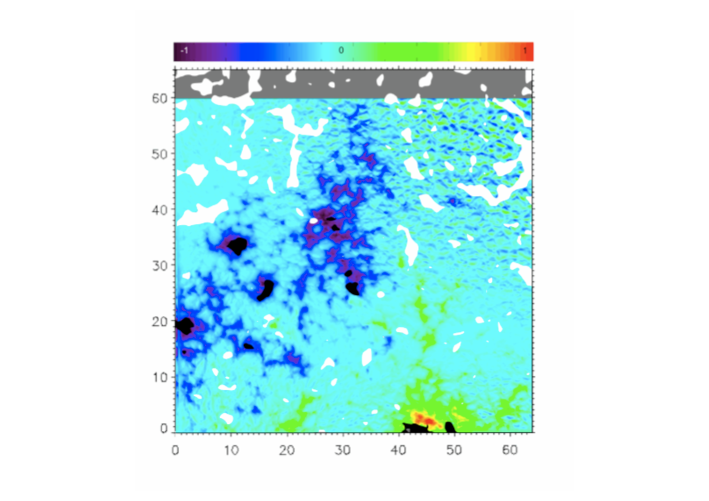 |
Figure 7 shows the location (white areas) of speeds
(velocity magnitudes) within three different ranges in km s-1, for the SST
data (the first series in Table 1): low velocity magnitudes
lower than 0.3, medium velocity magnitudes in the range 0.3 - 0.8 and large
velocity magnitudes greater than 0.8.
Small speeds are mainly grouped in the central part of the FOV where an intense
magnetic activity is detected as evidenced by the high concentration of G-band
bright points and faculae present in this region (see Fig. 1).
Around pores, the velocity magnitudes mainly correspond
to the lower range ( 0.3 km s-1) so that they are surrounded by
white areas in Fig. 7 (upper panel). The areas mapping
medium velocity magnitudes are regularly spread out all over the FOV except in
the proximity of pores as shown in Fig. 7 (middle panel).
Large velocities ( 0.8 km s-1) are not homogeneously distributed
in the FOV but mainly grouped at the two upper corners of Fig. 7 (lower panel).
The magnetogram in the last panel of Fig. 1 has
been overlapped to better identify the match between the locations displaying larger
velocity magnitudes and the less-magnetized regions (scaled as 0 and colored in light blue). These large flows zones might
reflect the presence of supergranular cells as commented in Sect. 3.1.
3.5 Velocity distribution around solar pores

From the computed velocity fields we can perform a detailed analysis of the
velocity distribution around the solar pores. To pursue this study we will use
the region observed with the SST where we have a useful collection of pores available
to work with. As we have two time series for this region (see Table 1),
we will employ the first one covering the longest time period, except for one of
the pores which is out of the FOV. For this pore, we will use the second time
series. Figure 8 shows the FOV including all the pores under
study which are labeled with consecutive numbers for easy identification
hereafter.

Figure 8 (lower panel) illustrates the projection of the
velocities into radial and transversal components as a convenient way to
compute inward and outward motions. The figure plots two points in the
granulation surrounding a solar pore with their corresponding velocity vectors
. The pore is centered at coordinates with respect to the
orthogonal coordinate system X,Y placed at the lower left corner of the FOV.
Vector is the position vector of a given point with respect to the
pore center. The pore center is located at its gravity-center calculated by
weighting the position of every point inside the pore with the inverse of its
respective intensity. Velocity vectors in every point of the granulation
surrounding the pore are projected into radial and transversal
components.
In order to establish the inward and outward motions, we first select the FOV
including the pore under study. Since active regions in general, and pores in
particular, exhibit their own displacement (due to differential rotation and
intrinsic motions) while embedded in the granulation pattern, we align the time
series with respect to an area framing the pore (correlation box) so that we
make sure we are measuring plasma motions with respect to the pore. We compute
the map of horizontal velocities by LCT with the same Gaussian tracking window
(FWHM 10) employed in the previous sections. The next step is to define
the "radial directions" (see lower panel in Fig. 8) that will
be used as the reference to project the velocities. For short distances these
directions are defined as perpendicular to the pore border. These perpendicular
directions are calculated from the gradients of intensity in a smoothed
pore-mask image22
2
A binary mask setting the area occupied by the pore
(1/0 inside/outside the pore) is defined. Then this mask is smoothed by
convolving with a Gaussian function so that we obtain a distribution of
pseudo-intensities smoothly ranging from 1 to 0 and describing a blurred shape
of the pore. This will be the smoothed pore-mask image to which we refer
above.. This way, one can also deal with non round-shaped pores. The limit for
short distances is defined by thresholding the intensity gradients. The
threshold depends on the pore shape and size. At large distances
(i.e. 3 times larger than the pore mean radius) all pores are considered as
round-shaped structures and the radial directions
are defined by the position vector of a given point with respect to
the pore center. According to the lower panel in Fig. 8,
inward/outward motions correspond to negative/positive, where
is the angle formed by and the positive radial direction
(outward) at each point of the FOV. The value of is mapped in gray
scale ranging from 1 for purely radial outward velocities (in black) to
-1 for purely inward velocities (in white). A binary mask is created
from the previous gray-scaled map where areas in black and white
correspond to velocities with positive (outward) and negative (inward) radial
components, respectively.

We apply the aforementioned method to our sample of 7 different pores shown in
the upper panel of Fig. 8. The results are displayed in
Fig. 9 where rows display the different pores and the
columns correspond to: 1) the averaged FOV around the pore; 2) the velocity
field; 3) the gray-scale representation of ; and 4) the final binary
representation mapping the areas with inward (white) and outward
(black) radial velocity components, after applying the binary mask. The
analysis of all cases establishes that the flows display a clear preference for
inward directions around the pores. This fact is systematically found in all
examples. The more regular-shaped pores are surrounded by an also regular
annular-like area with inward velocity components, having a mean width similar
to the center-to-border distance in the pore. The dividing line between inward
and outward motions is connecting the centers of divergence.
Fig. 10 (upper panels) shows color-scaled maps of the velocity
magnitudes (ranging from 0 to 1 km s-1) for the more regular-shaped pores
(1 and 2) in our sample, represented in the the two upper rows of
Fig. 9. Note that both pores exhibit proto-penumbral
structures which are also visible in other pores of the sample. The centers of
divergence are clearly identified in the maps of Fig. 10 as
black structures around the pores. Another important distinctive
feature in these maps is that the highest speeds are located beyond these black
structures away from the pore.
In an attempt to study a possible systematic trend in the variation of the speeds around the most regular-shaped pores having approximately the same size in our sample, as a first approach and for simplicity, we calculate the mean velocity magnitude in consecutive ribbons (strips) encircling the pores 1 and 2. A total of 12 adjacent ribbons ( 024 wide), referred to as ring-like structures surrounding the pore, are used for this analysis.
We emphasize that the following results should not be taken as trying to globalize the properties and behavior of the flows around all solar pores but as a preliminar and simplistic case in which we can compare two pores of our sample under similar conditions (size, shape, polarity among others) and apply the above-mentioned method of computing velocities in ribbons around them. In a future work we will conduct a study to be able to compare more general cases.
Figure 10 (lower panels) plots the speeds versus distance to the pore border. The velocity magnitudes increment as a function of this distance: 1) the mean value of speeds increments rapidly at distances ranging from 015 to 04; 2) in the range 04 - 10 the variation curve is flatter; 3) in the range 10 - 16 we again obtain very sharp increments. Up to this distance from the pore border, we observe the same behavior in both pores. Nevertheless, the mean speed values at 16 are quite different (250 vs. 390 m s-1). At further distances ( 16) the trend in the mean velocity magnitudes differs substantially. We must bear in mind that the flows around the pore can also be affected by the intrinsic characteristics of every single pore and by the contribution from other sources in the neighbourhood, e.g. pores in the vicinity.
4 Conclusions
The proper motions in solar active regions displaying pores are analyzed from
high-resolution time series of images. The observing material stems from
coordinated ground-based and space observations. Thus, part of this material
was acquired with the Swedish 1-m Solar Telescope, and reconstructed by
employing the novel MFBD and MOMFBD techniques to achieve image resolutions
near the diffraction limit. The other part of the data stems from the solar
telescope on board the Hinode satellite. The long duration, stability
and high-resolution of the time series achieved by Hinode enable us to
study dynamical properties of the photospheric horizontal flows along periods
of time much longer than those typically reachable from ground-based observations
which are restricted by varying seeing conditions.
The local correlation technique applied to the time series allowed us to track
the proper motions of structures in solar active regions and particularly in
the areas nearby solar pores. Proper motions have been tracked in a variety of
active regions for periods of typically 20-60 min but also one
for several hours. We conclude that the flow patterns derived from different
observational sets are consistent among each other in the sense that they show
the determinant and overall influence of exploding events in the granulation
around the pores and in the whole FOV. Motions toward the pores in their
nearest vicinity are the dominant characteristic we claim to observe
systematically. Thus, we do not find any trace of moat flow in the wide sample
of pores studied. The motions at the periphery of the pores are basically
influenced by the external plasma flows deposited by the exploding events, as
suggested by other authors in previous works (Sobotka et al., 1999; Roudier, Bonet & Sobotka, 2002; Sankarasubramanian & Rimmele, 2003).
In addition, the horizontal velocity magnitudes are clearly lower ( 0.3 km s-1)
in the nearest locations surrounding the pores and, in general, in the more magnetized regions
in the FOV, as expected due to the inhibition of convection taking place.
Our results are also in agreement with recently developed 3D radiative magnetohydrodynamic simulations of pore-like magnetic structures that report downflows surrounding them, maintained by
horizontal flows towards the simulated pore (Cameron et al., 2007). Moreover, we interpret the dividing line between radial inward and outward motions, found
by Deng et al. (2007) outside the residual pore in the last stage of a decaying
sunspot, as corresponding to the location of the centres of divergence of the
exploding events around the pore. The outward motions these authors describe,
which are not in the immediate surroundings of the pore but separated by the
annular inward motion, would then correspond not to moat flows but to the
outward flows originated in the regular mesh of divergence centers around the
pore.
Acknowledgements.
The Swedish 1-m Solar Telescope is operated in the island of La Palma by the Institute of Solar Physics of the Royal Swedish Academy of Sciences in the Spanish Observatorio del Roque de los Muchachos of the Instituto de Astrofísica de Canarias. We thank the scientists of the Hinode team for the operation of the instruments. Hinode is a Japanese mission developed and launched by ISAS/JAXA, with NAOJ as domestic partner and NASA and STFC (UK) as international partners. It is operated by these agencies in co-operation with ESA and NSC (Norway). The reconstruction of images using the MOMFBD technique is a very computationally expensive task. To reduce the time needed for it, we made use of the Condor workload management system (http://www.cs.wisc.edu/condor/). S. Vargas thanks the people from the Institute of Solar Physics in Stockholm for his support during his short-stay in Sweden. Partial support by the Spanish Ministerio de Ciencia e Innovación through projects ESP2006-13030-C06-01 and AYA2007-63881, and financial support by the European Commission through the SOLAIRE Network (MTRN-CT-2006-035484) are gratefulyReferences
- Cabrera Solana et al. (2006) Cabrera Solana, D., Bellot Rubio, L.R., Beck, C., Del Toro Iniesta, J.C., 2006, ApJ 649, L41
- Cameron et al. (2007) Cameron, R., Schüssler, M., Vögler, A., & Zakharov, V. 2007, A&A, 474, 261
- Deng et al. (2007) Deng, N., Choudhary, D.P., Tritschler, A., Denker, C., Liu, C., & Wang, H., 2007, ApJ 671, 1013
- Giordano et al. (2008) Giordano, S., Berrilli, F., Del Moro, D., Penza, V., 2008, A&A, 489, 747
- Hirzberger (2003) Hirzberger, J., 2003, A&A, 405, 331
- Keil (1999) Keil, S. L., Balasubramaniam, K. S., Smaldone, L. A., & Reger, B. 1999, ApJ, 510, 422
- Kosugi et al. (2007) Kosugi, T., Matsuzaki, K., Sakao, T., et al. 2007, Sol. Phys., 243, 3
- Löfdahl (1996) Löfdahl, M.G. 1996, Ph.D Thesis, Stockholm University, Stockholm (Sweden)
- Löfdahl (2002) Löfdahl, M.G., 2002, Proc. SPIE., 4792, P.146
- Molowny-Horas & Yi (1994) Molowny-Horas, R., & Yi, Z., 1994, ITA (Oslo) Internal Rep. No. 31
- November & Simon (1988) November, L.J., & Simon, G.W., 1988, ApJ 333, 427
- Roudier, Bonet & Sobotka (2002) Roudier, Th., Bonet, J.A., & Sobotka, M., 2002, A&A, 395, 249
- Sainz Dalda & Martínez Pillet (2005) Sainz Dalda, A., Martínez Pillet, V., 2005, ApJ, 662, 1176
- Sankarasubramanian & Rimmele (2003) Sankarasubramanian, K., & Rimmele, T. 2003, ApJ, 598, 689
- Scharmer et al. (2003a) Scharmer G. B., Bjelksjö K., Korhonen, T.K., Lindberg, B. & Petterson, B., 2003a, Proc. SPIE. 4853, 341
- Scharmer et al. (2003b) Scharmer G. B., Dettori, P. M., Löfdahl, M.G. , & Shand, M. 2003b, Proc. SPIE, 4853, 370
- Sobotka et al. (1999) Sobotka, M., Vázquez, M., Bonet, J.A., Hanslmeier, A., Hirzberger, J., 1999, ApJ, 511, 436
- Thomas & Weiss (2008) Thomas, J.H. & Weiss, N.O., 2008 in Sunspots and Starspots, Cambridge Astrophysics Series 46, CUP, Cambridge
- Title et al (1986) Title, A. M., Tarbell, T. D., Simon, G., and the SOUP team. 1986, Adv. Space Res., 6,253
- Tsuneta et al. (2008) Tsuneta, S., et al. 2008, Sol. Phys., 249, 167
- Van Noort, Rouppe van der Voort & Löfdahl (2005) Van Noort. M., Rouppe van der Voort, L., Löfdahl, M. G., 2005, Sol. Phys., 228, 191
- Vargas Domínguez et al. (2007) Vargas Domínguez, S., Bonet, J.A., Martínez Pillet, V., Katsukawa, Y., Kitakoshi, Y., Rouppe van der Voort, L., 2007, ApJ, 660, L165
- Vargas Domínguez et al. (2008) Vargas Domínguez, S., Rouppe van der Voort, L., Bonet, J.A., Martínez Pillet, V., van Noort, M., Katsukawa, Y. 2008, ApJ, 679, 900
- Vargas Domínguez (2008) Vargas Domínguez, S., 2008, PhD thesis, University of La Laguna - Instituto de Astrofísica de Canarias, Tenerife (Spain)
- Wang & Zirin (1992) Wang, H., & Zirin, H. 1992. Sol. Phys., 140, 41
- Zuccarello et al. (2009) Zuccarello, F., Romano, P., Guglielmino, S.L., Centrone, M., Criscuoli, S., Ermolli, I., Berrilli, F., Del Moro, D., 2009, A&A, 500, L5