Physical picture, pattern-control, and detection approach for tightly focused beams: In the view of Fourier optics
Daquan Lu, and Wei Hu
Laboratory of Photonic Information Technology, South
China Normal University, Guangzhou 510631, China
Abstract
We investigate the mechanism of the nonparaxial propagation of the tightly focused beams in the view of Fourier optics. It shows that it is the phase of the angular spectrum which induces the interesting evolution of the tightly focused beams. Based on the theory of Fourier optics, we propose an approach on controlling and detecting the focusing spot of the tightly focused beams.
It is well-known that there are two types of propagation theory for laser beams, i.e. the paraxial propagation theory and the nonparaxial propagation theory. The paraxial theory is able to give an accurate description while the divergence angles of beam is very small and the beam width is much larger than its wavelength. However, if a beam is with a large divergence angle or is tightly focused, the paraxial approximation is invalid and it requires a non-paraxial correction to the paraxial solution.
In the past decades, the paraxial diffraction equation has been thoroughly investigated. Various types of beam solutions with different transverse profiles have been obtained in Cartesian, circular cylindrical, and elliptical coordinates (e.g., [1, 2, 3] and references therein). These solutions can be roughly classified into two types: i) shape-invariant beams, such as LG, HG, and IG beams; and ii) shape-variant beams, such as higher-order elegant-Hermite-Gaussian (EHG), elegant-Laguerre-Gaussian (ELG), and elegant-Ince- Gaussian (EIG) beams. The propagation of these beams has been investigated in detail and many parameters, such as width, divergence, radius of curvature, and quality factor, have been introduced to describe their propagation. In summary, the theory of paraxial propagation has been well developed over the past decades. On the other hand, there are also various approaches for the nonparaxial propagation of beams[4, 5, 6, 7, 8, 9]. However, because of the complexity of the nonparaxial wave equation, the mechanism for the beam evolution under the nonparaxial condition is still unclarified.
In this paper, we investigate the mechanism of the nonparaxial propagation in the view of Fourier optics. It shows that it is the phase of the angular spectrum which induces the interesting evolution of the tightly focused beams. Based on the theory of Fourier optics, we propose an approach on controlling and detecting the focusing spot of the tightly focused beams.
The studies of this paper is based on the scalar wave equation,
| (1) |
which describes the evolution of the electromagnetic field in free space. However, it is well known that, outside the realm of paraxial approximation, the electromagnetic field have to be handled as a vectorial one since the coupling between each components. And the longitudinal component is not negligible for a nonparaxial pulsed beam. Fortunately, in free space, the longitudinal component can be evaluated from the knowledge of the transverse part, i.e., base on the relation . In this perspective and also for conciseness, we only consider the transverse components of the electromagnetic field and our results are limited to the scalar field in this paper.
A scalar laser field can be regarded as the superposition of various planar waves which propagate in different directions. Every plane wave experiences a corresponding phase shift when a plane wave propagate from to :
| (2) |
where , , . At the plane , the linear superposition of all spectrums yields the field in spatial domain, i.e.
| (3) |
Equation (3) is tantamount to
| (4) |
where operators and represent the Fourier transform and the inverse Fourier transform, respectively. Therefore, in the view of Fourier optics, the nonparaxial propagation from to results from three steps: i) transform the field at , i.e., , to the angular spectrum domain; ii) add a phase on ; iii) inversely transform the angular spectrum at to the spatial domain.
During propagation, the second step plays an important role since different angular-spectral components experience different phase shift . In fact, we can borrow the ideal of the dispersion of a pulse in fiber to analyze the influence of the difference of the phase shift on the evolution of the beam. We make a Taylor expansion on and have
| (5) |
where
| (6) |
As shown in Eq. (5), the beam experiences the spatial dispersion during propagation. It is noted that there are two critical difference between the temporal dispersion of the pules in fiber and the spatial dispersion of the beam in free space: i) The beam experiences only even-order spatial dispersion, whereas the pulse experiences both even- and odd-order temporal dispersion. ii)For different media of the fiber and wavelengths of the pulse, the temporal dispersion in fiber can be positive or negative, and the dispersion with different orders can be with different signal. However for the diffraction of the beam in free space, the signal of all orders of spatial dispersion () are negative, which means the higher spatial frequency experiences lager phase-shift than the lower spatial frequency. During propagation, all orders of spatial dispersion together cause a negative spatial chirp (or in other words, a convex copahsal surface).
If the beam width is much larger than the wave lenth and the divergence angle is very small (or in other words, the paraxial approximation is satisfied), the angular-spectral width so narrow that only the lowest dispersion is necessary to be taken into account. under this condition Eq. (4) reduces to
| (7) |
Eqation (7) is called the Fresnel integral, which governs the evolution of an arbitrary paraxial beam.
Whereas, if the beam is so narrow that the beam width is comparable with the wavelength or the divergency angle is very large so that the angular-spectral width is no longer small enough to justify the truncation of the expansion (5) after the term, the higher orders of dispersion should be included in the expansion. And Eq. (3) deduces to
| (8) |
Eq. (8) describes the propagation of the nonparaxial beams, such as the largely divergent beams from the sources whose size is about the wavelength and the tightly focused beams.
In the following, we will discuss the influence of different orders of spatial dispersion on the propagation of a tighyly focused beam. In application, the paraboloids or the spherical lenses provide positive linear spatial chirp and are frequently used to focus a beam; and the field next to the lens is with a concave spherical cophasal surface. In the framework of the paraxial theory, there are two key characters of the propagation. i) The evolution of the beam is induced only by the 2nd order spatial dispersion, which does not vary the angular spectrum distribution, but induces a spherical phase distribution in the angular spectrum domain during propagation. In the view of Fourier Optics, the Hermite-, laguerre-, and Ince-Gaussian functions are the eigen functions with spherical cophasal surface of the Fourier transform, i.e.
| (9) |
where represents an arbitrary Hermite-, laguerre-, or Ince-Gaussian function. Therefore, an arbitrary beam, which is resulted from the linear superposition of these three types of beams with the same waist location and Rayleigh distance, would remain shape-invariant during propagation under the paraxial approximation. The paraxial propagation varies only the beam width and the radius of the cophasal surface. ii) Because only the 2nd order spatial dispersion is taken into account and the higher orders of dispersion are neglected, the dispersion-induced negative linear chirp can completely cancel the initial positive linear chirp at a certain plane. According to Eq. (3), at that plane the beam width is Fourier-Transform-limited and arrives its minimum, thus that plane becomes the waist of the focused beam; and the intensity distribution is symmetric about the waist (we will call it the pseudo-waist in the following, because it is not really the waist for the tightly focused case).


However, in fact the paraxial theory becomes invalid for the tightly
focused beams, because under this condition the higher-orders of
spatial dispersion play critical roles in the evolution of the beam.
A tightly focused beam presents interesting evolution which is
critically different to the paraxial anticipation:
I) In the view of
Fourier optics, the higher-order spatial dispersion induces the
addition of the fourth- and higher£order phase factor in the
angular spectrum domain. mathematically, each Hermite-, Laguerre-,
or Ince-Gaussian functions with such a phase factors are no longer
the eigen functions of Fourier transform. Therefore any paraxially
shape-invariant beams becomes shape-variant under the nonparaxial
condition (e.g. the tightly focused fundmental Gaussian beam Shown
in Fig. 1).
II) At the pseudo-waist, the linear initial positive chirp only
balances the 2nd-order-spatial-dispersion-induced negative chirp.
The higher-orders of spatial dispersion, which induces a nonlinear
negative chirp, would broadens the beam.The beam width is larger
than the Fourier-Transform-limited one predicted by the paraxial
theory. The farther the focusing plane is from the pseudo-waist, the
larger the chirp will be, and in turn the larger the beam width will
be resulted (Fig. 2).
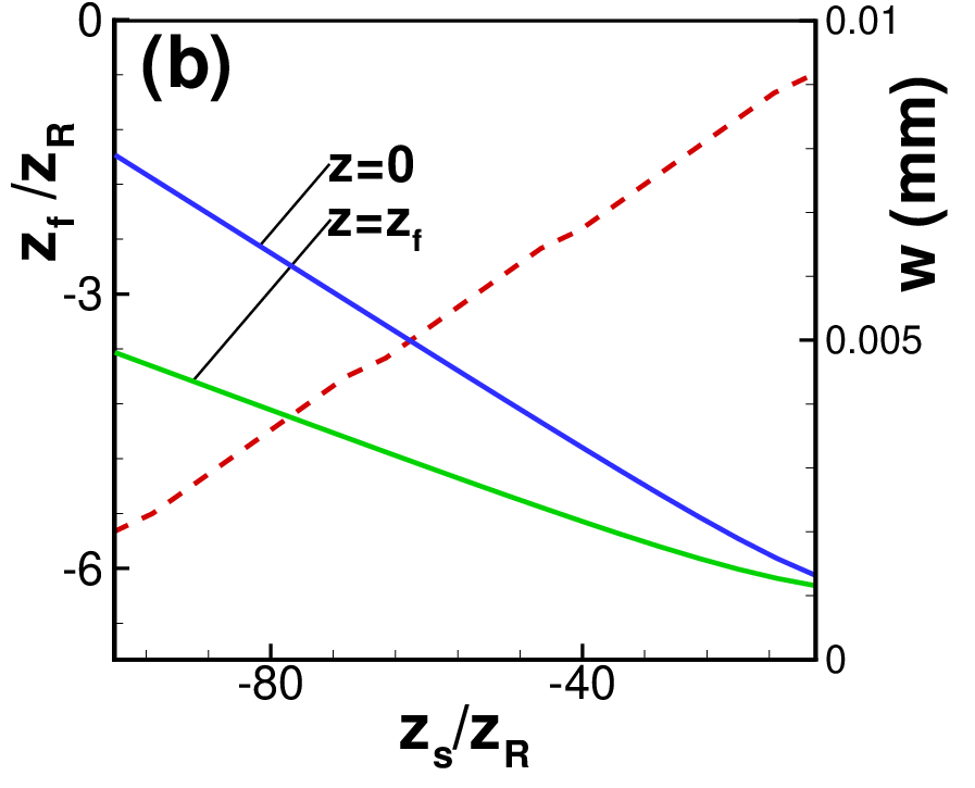
III) There is a plane where the chirp-induced broadening of beam width is
smallest (which is still larger than the Fourier-Transform-limited
one). If we call this real-waist, the real-waist becomes farther and
father from the pseudo-waist with the increase of the distance
between the focusing plane and the pseudo-waist (Fig. 2).
IV) The chirp is asymmetric about the pseudo-waist, therefore
neither the pattern nor the beam width is symmetric about the
pseudo-waist. For the Gaussian beam, for example, at the planes
after the pseudo-waist the phase in angular spectrum domain
decreases monotonically with and result in an negative and
nonlinear chirp. Therefore the beam is wider than what predicted by
the paraxial theory. At some planes before the pseudo-waist, the
phase in angular spectrum domain dose not vary monotonically with
and results in an s-like distribution of the chirp. Therefore,
at such a plane there is the same chirp occurs at two values of
. These two angular spectrum interfere constructively or
destructively, depending on their relative phase difference. The
interference then results in a multi-ringed distribution of the beam
in the spatial domain.

Although these phenomena are interesting, they frequently occur negative impact on real applications of the tightly focused beams. In many applications, such as the laser-electron acceleration and the trapping and manipulation of atom, the tightly focused beam is expected to have the following properties: i)the spot size is the smallest one to have the highest intensity; ii)the real-waist is locate at the pseudo-waist, for the convenience of the controling of the interaction. iii) the pattern at the real-waist is the same as that at the focusing plane, for the convenient of the beam shaping. Then a question arises: can we design the evolution of the tightly focused beam to satisfy the above requirements? The answer is yes. In fact, we can do this by modulate the forth- and higher-order spatial dispersion. For example, if the field at the focusing plane is the distance between the focusing plane and the pseudo-waist is , we can pre-add a chirp on the beam at the focusing plane, i.e.
| (10) |
then the field at the pseudo-waist plane becomes
| (11) | |||||
| (12) |
which is identical to that resulted from the paraxial propagation. Therefore, if is the Hermite-, laguerre-, or Ince-Gaussian beams or the linear superposition of them, the shape of the field at the pseudo-waist plane is the same as . The width is the minimum; and the pseudo-waist then becomes the real-waist (Fig. 3).
For a tightly focused beam, the beam width can be focused to the size of or even sub-. For such a narrow beam, even the knife-edge based beam profilers is difficult to directly get the precise intensity distribution. On the other hand, If a traditional 4f system, which works well only in the paraxial condition, is directly introduced to amplify the pattern, the nonparaxiality would made the detected result deviate from the real intensity distribution. But based on the higher-order phase modulation, just like the method in the above paragraph, we can get the shape invariant and amplified intensity distribution. As a result, even a charge-coupled-device camera can precisely detect the intensity distribution through this approach.
In conclusion, the evolution of the tightly focused beams can be explained with the theory of Fourier optics. In the propagation of the tightly focused beam, the phase distribution in the angular spectrum domain plays an important role and induces interesting beam patterns. By modulating the phase distribution in the angular spectrum domain, one can made the field at the pseudo-waist plane identical to that resulted from the paraxial propagation, of which the width is the minimum and the pseudo-waist is located at the real-waist. In the same approach, the intensity distribution of the focused field can remain shape invariant and be amplified so that even a charge-coupled-device camera can precisely detect the intensity distribution.
References
- [1] M. A. Bandres and J. C. Gutiérrez-Vega, Opt. Lett., 32 (2007) 3459.
- [2] M. A. Bandres and J. C. Gutiéerrez-Vega, Opt. Lett., 33 (2008) 177.
- [3] M. A. Bandres and J. C. Gutiéerrez-Vega, Proc. SPIE, 6290 (2006) 62900S.
- [4] M. Lax, W.H. Louisell, W.B. Mcknight, Phys. Rev. A (1975) 1365.
- [5] Q. Cao, X. Deng, J. Opt. Soc. Am. A 15 (5) (1998) 1144.
- [6] Q. Cao, X. Deng, J. Opt. Soc. Am. A 16 (10) (1999) 2494.
- [7] X. Fu, H. Guo, W. Hu, Phys. Rev. E 65 (2002) 056611.
- [8] M. Trippenbach, T.C. Scott, Y.B. Band, Opt. Lett. 22 (1997) 579.
- [9] S. Blair, K. Wagner, Opt. Quantum Electron. 30 (1998) 697.