Inverse Folding of RNA Pseudoknot Structures
Abstract
Background:
RNA exhibits a variety of structural configurations. Here we consider a structure to be tantamount to the noncrossing Watson-Crick and G-U-base pairings (secondary structure) and additional cross-serial base pairs. These interactions are called pseudoknots and are observed across the whole spectrum of RNA functionalities. In the context of studying natural RNA structures, searching for new ribozymes and designing artificial RNA, it is of interest to find RNA sequences folding into a specific structure and to analyze their induced neutral networks. Since the established inverse folding algorithms, RNAinverse, RNA-SSD as well as INFO-RNA are limited to RNA secondary structures, we present in this paper the inverse folding algorithm Inv which can deal with -noncrossing, canonical pseudoknot structures.
Results:
In this paper we present the inverse folding algorithm Inv. We give a detailed analysis of Inv, including pseudocodes. We show that Inv allows to design in particular -noncrossing nonplanar RNA pseudoknot -noncrossing RNA structures–a class which is difficult to construct via dynamic programming routines. Inv is freely available at http://www.combinatorics.cn/cbpc/inv.html.
Conclusions:
The algorithm Inv extends inverse folding capabilities to RNA pseudoknot structures. In comparison with RNAinverse it uses new ideas, for instance by considering sets of competing structures. As a result, Inv is not only able to find novel sequences even for RNA secondary structures, it does so in the context of competing structures that potentially exhibit cross-serial interactions.
1 Introduction
Pseudoknots are structural elements of central importance in RNA structures [1], see Figure 1. They represent cross-serial base pairing interactions between RNA nucleotides that are functionally important in tRNAs, RNaseP [2], telomerase RNA [3], and ribosomal RNAs [4]. Pseudoknot structures are being observed in the mimicry of tRNA structures in plant virus RNAs as well as the binding to the HIV-1 reverse transcriptase in in vitro selection experiments [5]. Furthermore basic mechanisms, like ribosomal frame shifting, involve pseudoknots [6].

Despite them playing a key role in a variety of contexts, pseudoknots are excluded from large-scale computational studies. Although the problem has attracted considerable attention in the last decade, pseudoknots are considered a somewhat “exotic” structural concept. For all we know [8], the ab initio prediction of general RNA pseudoknot structures is NP-complete and algorithmic difficulties of pseudoknot folding are confounded by the fact that the thermodynamics of pseudoknots is far from being well understood.
As for the folding of RNA secondary structures, Waterman et al [9, 10], Zuker et al [11] and Nussinov [12] established the dynamic programming (DP) folding routines. The first mfe-folding algorithm for RNA secondary structures, however, dates back to the 60’s [13, 14, 15]. For restricted classes of pseudoknots, several algorithms have been designed: Rivas and Eddy [16], Dirks and Pierce[17], Reeder and Giegerich [18] and Ren et al [19]. Recently, a novel ab initio folding algorithm Cross has been introduced [20]. generates minimum free energy (mfe), -noncrossing, -canonical RNA structures, i.e. structures that do not contain three or more mutually crossing arcs and in which each stack, i.e. sequence of parallel arcs, see eq. (1), has size greater or equal than three. In particular, in a -canonical structure there are no isolated arcs, see Figure 2.

The notion of mfe-structure is based on a specific concept of pseudoknot loops and respective loop-based energy parameters. This thermodynamic model was conceived by Tinoco and refined by Freier, Turner, Ninio, and others [14, 21, 22, 23, 24, 25].
1.1 -noncrossing, -canonical RNA pseudoknot structures
Let us turn back the clock: three decades ago Waterman et al. [26], Nussinov et al. [12] and Kleitman et al. in [27] analyzed RNA secondary structures. Secondary structures are coarse grained RNA contact structures, see Figure 3.

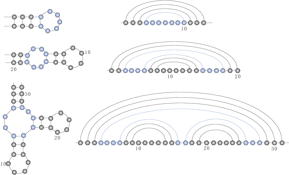
Secondary structures can be represented as diagrams, i.e. labeled graphs over the vertex set with vertex degrees , represented by drawing its vertices on a horizontal line and its arcs (), in the upper half-plane, see Figure 1 and Figure 4.
Here, vertices and arcs correspond to the nucleotides A, G, U, C and Watson-Crick (A-U, G-C) and (U-G) base pairs, respectively.
In a diagram, two arcs and are called crossing if holds. Accordingly, a -crossing is a sequence of arcs such that , see Figure 5.


We call diagrams containing at most -crossings, -noncrossing diagrams. RNA secondary structures have no crossings in their diagram representation, see Figure 3 and Figure 4, and are therefore -noncrossing diagrams. A structure in which any stack has at least size is called -canonical, where a stack of size is a sequence of “parallel” arcs of the form
| (1) |
As a natural generalization of RNA secondary structures -noncrossing RNA structures [28, 29, 30] were introduced. A -noncrossing RNA structure is -noncrossing diagram without arcs of the form . In the following we assume , i.e. in the diagram representation there are at most two mutually crossing arcs, a minimum arc-length of four and a minimum stack-size of three base pairs. The notion -noncrossing stipulates that the complexity of a pseudoknot is related to the maximal number of mutually crossing bonds. Indeed, most natural RNA pseudoknots are -noncrossing [31].
1.2 Neutral networks
Before considering an inverse folding algorithm into specific RNA structures one has to have at least some rationale as to why there exists one sequence realizing a given target as mfe-configuration. In fact this is, on the level of entire folding maps, guaranteed by the combinatorics of the target structures alone. It has been shown in [32], that the numbers of -noncrossing RNA pseudoknot structures, satisfying the biophysical constraints grows asymptotically as , where is some explicitly known constant. In view of the central limit theorems of [33], this fact implies the existence of extended (exponentially large) sets of sequences that all fold into one -noncrossing RNA pseudoknot structure, . In other words, the combinatorics of -noncrossing RNA structures alone implies that there are many sequences mapping (folding) into a single structure. The set of all such sequences is called the neutral network11 1 the term “neutral network” as opposed to “neutral set” stems from giant component results of random induced subgraphs of -cubes. That is, neutral networks are typically connected in sequence space of the structure [34, 35], see Figure 6.

By construction, all the sequences contained in such a neutral network are all compatible with . That is, at any two positions paired in , we find two bases capable of forming a bond (A-U, U-A, G-C, C-G, G-U and U-G), see Figure 7. Let be a sequence derived via a mutation22 2 note: we do not consider insertions or deletions. of . If is again compatible with , we call this mutation “compatible”.

Let denote the set of -compatible sequences. The structure motivates to consider a new adjacency relation within . Indeed, we may reorganize a sequence into the pair
| (2) |
where the denotes the unpaired nucleotides and the denotes base pairs, respectively, see Figure 7. We can then view and as elements of the formal cubes and , implying the new adjacency relation for elements of .
Accordingly, there are two types of compatible neighbors in the sequence space - and -neighbors: a -neighbor has Hamming distance one and differs exactly by a point mutation at an unpaired position. Analogously a -neighbor differs by a compensatory base pair-mutation, see Figure 8.

Note, however, that a p-neighbor has either Hamming distance one () or Hamming distance two (). We call a u- or a p-neighbor, , a compatible neighbor. In light of the adjacency notion for the set of compatible sequences we call the set of all sequences folding into the neutral network of . By construction, the neutral network of is contained in . If is contained in the neutral network we refer to as a neutral neighbor. This gives rise to consider the compatible and neutral distance of the two sequences, denoted by and . These are the minimum length of a -path and path in the neutral network between and , respectively. Note that since each neutral path is in particular a compatible path, the compatible distance is always smaller or equal than the neutral distance.
In this paper we study the inverse folding problem for RNA pseudoknot structures: for a given -noncrossing target structure , we search for sequences from , that have as mfe configuration.
2 Background
For RNA secondary structures, there are three different strategies for inverse folding, RNAinverse, RNA-SSD and INFO-RNA [36, 37, 38],
They all generate via a local search routine iteratively sequences, whose structures have smaller and smaller distances to a given target. Here the distance between two structures is obtained by aligning them as diagrams and counting “”, if a given position is either unpaired or incident to an arc contained in both structures and “”, otherwise, see Figure 9.

One common assumption in these inverse folding algorithms is, that the energies of specific substructures contribute additively to the energy of the entire structure. Let us proceed by analyzing the algorithms.
RNAinverse
is the first inverse-folding algorithm that derives sequences that realize given RNA secondary structures as mfe-configuration. In its initialization step, a random compatible sequence for the target is generated. Then RNAinverse proceeds by updating the sequence to step by step, minimizing the structure distance between the mfe structure of and the target structure . Based on the observation, that the energy of a substructure contributes additively to the mfe of the molecule, RNAinverse optimizes “small” substructures first, eventually extending these to the entire structure. While optimizing substructures, RNAinverse does an adaptive walk in order to decrease the structure distance. In fact, this walk is based entirely on random compatible mutations.
RNA-SSD
RNA-SSD first assigns specific probabilities to the bases located in unpaired positions and the base pairs () of , respectively. In this assignment the probability of a unpaired position being assigned either A or U is greater than assigning G or C. Similarly, the probability of pairs G-C and C-G base pairs is greater than that of the other base pairs. Then, RNA-SSD derives a hierarchical decomposition of the target structure. It recursively splits the structure and thereby derives a binary decomposition tree rooted in and whose leaves correspond to -substructures. Each non-leaf node of this tree represents a substructure obtained by merging the two substructures of its respective children. Given this tree, RNA-SSD performs a stochastic local search, starting at the leaves, subsequently working its way up to the root.
INFO-RNA
employs a dynamic programming method for finding a well suited initial sequence. This sequence has a lowest energy with respect to the . Since the latter does not necessarily fold into , (due to potentially existing competing configurations) INFO-RNA then utilizes an improved33 3 relative to the local search routine used in RNAinverse stochastic local search in order to find a sequence in the neutral network of . In contrast to RNAinverse, INFO-RNA allows for increasing the distance to the target structure. At the same time, only positions that do not pair correctly and positions adjacent to these are examined.
2.1
is an ab initio folding algorithm that maps RNA sequences into -noncrossing RNA structures. It is guaranteed to search all -noncrossing, -canonical structures and derives some (not necessarily unique), loop-based mfe-configuration. In the following we always assume . The input of is an arbitrary RNA sequence and an integer . Its output is a list of -noncrossing, -canonical structures, the first of which being the mfe-structure for . This list of structures is ordered by the free energy and the first list-element, the mfe-structure, is denoted by . If no is specified, assumes as default.
Cross generates a mfe-structure based on specific loop-types of -noncrossing RNA structures. For a given structure , let be an arc contained in (-arc) and denote the set of -arcs that cross by .
For two arcs and , we next specify the partial order “” over the set of arcs:
All notions of minimal or maximal elements are understood to be with respect to . An arc is called a minimal, -crossing if there exists no such that . Note that can be minimal -crossing, while is not minimal -crossing. -noncrossing diagrams exhibit the following four basic loop-types:
(1)
A hairpin-loop is a pair
where is an arc and is an interval, i.e. a sequence of consecutive vertices .
(2)
An interior-loop, is a sequence
where is nested in . That is we have .
(3)
A multi-loop, see Figure 10 [20], is a sequence
where denotes a pseudoknot structure over (i.e. nested in ) and subject to the following condition: if all , i.e. all substructures are just arcs, for all , then we have ).

(P1)
A set of arcs
where and , such that
- (i)
the diagram induced by the arc-set is irreducible, i.e. the dependency-graph of (i.e. the graph having as vertex set and in which and are adjacent if and only if they cross) is connected and
- (ii)
for each there exists some arc (not necessarily contained in ) such that is minimal -crossing.
(P2)
Any , not contained in hairpin-, interior- or multi-loops.
Having discussed the basic loop-types, we are now in position to state
Theorem 1
Any -noncrossing RNA pseudoknot structure has a unique loop-decomposition [20].
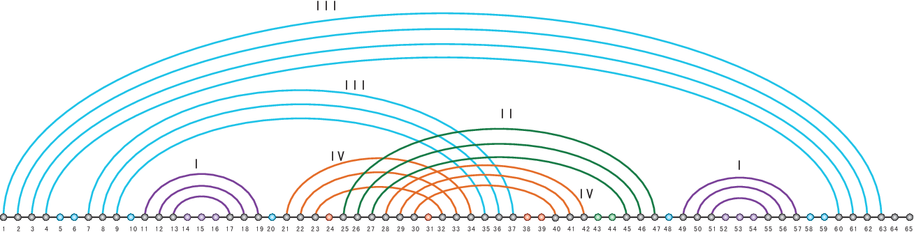
Figure 12 illustrates the loop decomposition of a -noncrossing structure.
A motif in is a -noncrossing structure, having only -maximal stacks of size exactly , see Figure 13. A skeleton, , is a -noncrossing structure such that
- •
its core, has no noncrossing arcs and
- •
its -graph, is connected.
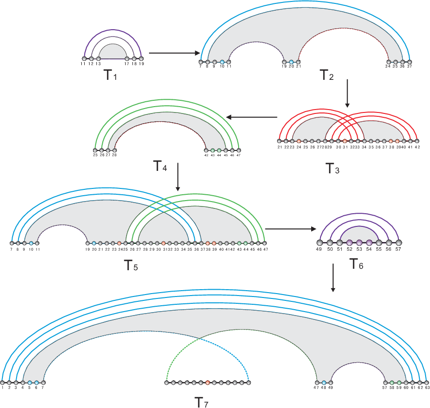
Here the core of a structure, , is obtained by collapsing its stacks into single arcs (thereby reducing its length) and the graph is obtained by mapping arcs into vertices and connecting any two if they cross in the diagram representation of , see Figure 14. As for the general strategy, constructs -noncrossing RNA structure “from top to bottom” via three subroutines:


I (Shadow):
Here we generate all maximal stacks of the structure. Note that a stack is maximal with respect to if it is not nested in some other stack. This is derived by “shadowing” the motifs, i.e. their -stacks are extended “from top to bottom”.
II (SkeletonBranch):
Given a shadow, the second step of consists in generating, the skeleta-tree. The nodes of this tree are particular -noncrossing structures, obtained by successive insertions of stacks. Intuitively, a skeleton encapsulates all cross-serial arcs that cannot be recursively computed. Here the tree complexity is controlled via limiting the (total) number of pseudoknots.
III (Saturation):
In the third subroutine each skeleton is saturated via DP-routines. After the saturation the mfe--noncrossing structure is derived.
Figure 15 provides an overview on how the three subroutines are combined.

3 The algorithm
The inverse folding algorithm Inv is based on the ab
initio folding algorithm . The input of is the target
structure, . The latter is expressed as a character string of
“:()[]{}”, where “:” denotes unpaired base and
“()”, “[]”, “{}” denote paired bases.
In Algorithm 1, we present the pseudocodes of algorithm . After validation of the target structure (lines to in Algorithm 1), similar to INFO-RNA, Inv constructs an initial sequence and then proceeds by a stochastic local search based on the loop decomposition of the target. This sequence is derived via the routine . We then decompose the target structure into loops and endow these with a linear order. According to this order we use the routine in order to find for each loop a “proper” local solution.
:()[]{}”
3.1 Adjust-Seq
In this section we describe Steps and of the pseudocodes presented in Algorithm 1. The routine , see line , generates a random sequence, , which is compatible to the target, with uniform probability.
We then initialize the variable via the sequence and set the variable , where denotes the structure distance between and .
Given the sequence , we construct a set of potential “competitors”, , i.e. a set of structures suited as folding targets for . In Algorithm 2 we show how to adjust the start sequence using the routine . Lines to of Algorithm 2, contain a For-loop, executed at most times. Here the loop-length is heuristically determined.
Setting the -parameter44 4 For all computer experiments we set ., , the subroutine executed in the loop-body consists of the following three steps.
Step I. Generating via .
Suppose we are in the th step of the For-loop and are given the sequence where . We consider , i.e. the list of suboptimal structures with respect to ,
If , then Inv returns . Else, in case of , we set
Otherwise we do not update and go directly to Step II.
Step II. The competitors.
We introduce a specific procedure that “perturbs” arcs of a given RNA pseudoknot structure, . Let be an arc of and let , denote the start- and end-point of . A perturbation of is a procedure which generates a new arc , such that
Clearly, there are nine perturbations of any given arc (including itself), see Figure 16.
We proceed by keeping , replacing the arc by a nontrivial perturbation or remove , arriving at a set of ten structures .

Now we use this method in order to generate the set by perturbing each arc of each structure . If has arcs, , then
This construction may result in duplicate, inconsistent or incompatible structures. Here, a structure is inconsistent if there exists at least one position paired with more than one base, and incompatible if there exists at least one arc not compatible with , see Figures 17 and 18. Here compatibility is understood with respect to the Watson-Crick and - base pairing rules. Deleting inconsistent and incompatible structures, as well as those identical to the target, we arrive at the set of competitors,


Step III. Mutation
Here we adjust with respect to as well as the set of competitors, derived in the previous step. Suppose . Let be the position paired to the position in the RNA structure , or 0 if position is unpaired. For instance, in Figure 19, we have , and . For each position of the target , if there exists a structure such that (see positions , , , and in Figure 19) we modify as follows:
- 1.
unpaired position: If , we update randomly into the nucleotide , such that for each , either or is not compatible with where , See position in Figure 19.
- 2.
start-point: If , set . We randomly choose a compatible base pair different from , such that for each , either or is not compatible with , where is the end-point paired with in (Figure 19: . The pair G-C retains the compatibility to , but is incompatible to ). By Figure 20 we show feasibility of this step.
- 3.
end-point: If , then by construction the nucleotide has already been considered in the previous step.

Therefore, updating all the nucleotides of , we arrive at the new sequence .
Note that the above mutation steps heuristically decrease the structure distance. However, the resulting sequence is not necessarily incompatible to all competitors. For instance, consider a competitor whose arcs are all contained . Since is compatible with , is compatible with . Since competitors are obtained from suboptimal folds such a scenario may arise.
In practice, this situation represents not a problem, since these type of competitors are likely to be ruled out by virtue of the fact that they have a mfe larger than that of the target structure.
Accordingly we have the following situation, competitors are eliminated due to two, equally important criteria: incompatibility as well as minimum free energy considerations.
If the distance of to is less than or equal to , we return to Step I (with ). Otherwise, we repeat Step III (for at most 5 times) thereby generating and set where is minimal.
The procedure employs the negative paradigm [17] in order to exclude energetically close conformations. It returns the sequence which is tailored to realize the target structure as mfe-fold.
3.2 Decompose and Local-Search
In this section we introduce two the routines, Decompose and Local-Search. The routine partitions into linearly ordered energy independent components, see Figure 12 and Section 2.1. Local-Search constructs iteratively an optimal sequence for via local solutions, that are optimal to certain substructures of .
: Suppose is decomposed as follows,
where the are the loops together with all arcs in the associated stems of the target.
We define a linear order over as follows: if either
- 1.
is nested in , or
- 2.
the start-point of precedes that of .
Next we define the interval
projecting the loop onto the interval and , being the maximal interval consisting of and its adjacent unpaired consecutive nucleotides, see Figure 12. Given two consecutive loops , we have two scenarios:
Let , then we have the sequence of intervals . If there are no unpaired nucleotides adjacent to , then and we simply delete all such . Thereby we derive the sequence of intervals . In Figure 22 we illustrate how to obtain this interval sequence: here the target decomposes into the loops , and we have , , , and .

: Given the sequence of intervals . We proceed by performing a local stochastic search on the subsequences (initialized via and where ). When we perform the local search on , only positions that contribute to the distance to the target, see Figure 9, or positions adjacent to the latter, will be altered. We use the arrays , to store the unpaired and paired positions of . In this process, we allow for mutations that increase the structure distance by five with probability . The latter parameter is heuristically determined. We iterate this routine until the distance is either zero or some halting criterion is met.
4 Discussion
The main result of this paper is the presentation of the algorithm Inv, freely available at
http://www.combinatorics.cn/cbpc/inv.html
Its input is a -noncrossing RNA structure , given in terms of its base pairs (where ). The output of Inv is an RNA sequences , where with the property , see Figure 23.

The core of Inv is a stochastic local search routine which is based on the fact that each -noncrossing RNA structure has a unique loop-decomposition, see Theorem 1 in Section 2.1. Inv generates “optimal” subsequences and eventually arrives at a global solution for itself. Inv generalizes the existing inverse folding algorithm by considering arbitrary -noncrossing canonical pseudoknot structures. Conceptually, Inv differs from INFO-RNA in how the start sequence is being generated and the particulars of the local search itself.
As discussed in the introduction it has to be given an argument as to why the inverse folding of pseudoknot RNA structures works. While folding maps into RNA secondary structures are well understood, the generalization to -noncrossing RNA structures is nontrivial. However the combinatorics of RNA pseudoknot structures [28, 29, 40] implies the existence of large neutral networks, i.e. networks composed by sequences that all fold into a specific pseudoknot structure. Therefore, the fact that it is indeed possible to generate via Inv sequences contained in the neutral networks of targets against competing pseudoknot configurations, see Figure 23 and Figure 24 confirms the predictions of [32].

An interesting class are the -noncrossing nonplanar pseudoknot structures. A nonplanar pseudoknot structure is a -noncrossing structure which is not a bi-secondary structure in the sense of Stadler [31]. That is, it cannot be represented by noncrossing arcs using the upper and lower half planes. Since DP-folding paradigms of pseudoknots folding are based on gap-matrices [16], the minimal class of ‘‘missed’’ structures55 5 given the implemented truncations are exactly these, nonplanar, -noncrossing structures. In Figure 25 we showcase a nonplanar RNA pseudoknot structure and sequences of its neutral network, generated by Inv.
As for the complexity of Inv, the determining factor is the subroutine . Suppose that the target is decomposed into intervals with the length , …, . For each interval, we may assume that line of runs for times, and that line is executed for times. Since will stop (line ) if ( line ), the remainder of , i.e. lines to run for times, each such execution having complexity . Therefore we arrive at the complexity
where denotes the complexity of the . The multiplicities and depend on various factors, such as , the random order of the elements of , (see Algorithm 3) and the probability . According to [33] the complexity of is and accordingly the complexity of is given by
In Figure 26 we present the average inverse folding time of several natural RNA structures taken from the PKdatabase [42]. These averages are computed via generating sequences of the target’s neutral networks. In addition we present in Table 1 the total time for executions of Inv for an additional set of RNA pseudoknot structures.


5 Competing interests
The authors declare that they have no competing interests.
6 Authors contributions
All authors contributed equally to this paper.
7 Acknowledgments
We are grateful to Fenix W.D. Huang for discussions. Special thanks belongs to the two anonymous referee’s whose thoughtful comments have greatly helped in deriving an improved version of the paper. This work was supported by the Project, the PCSIRT of the Ministry of Education, the Ministry of Science and Technology, and the National Science Foundation of China.
References
- [1] Westhof E, Jaeger L: RNA pseudoknots. Curr Opin Struct Biol 1992, 2(3):327–333.
- [2] Loria A, Pan T: Domain structure of the ribozyme from eubacterial ribonuclease P. RNA 1996, 2:551–563.
- [3] Staple DW, Butcher SE: Pseudoknots: RNA structures with diverse functions. PLoS Biol 2005, 3(6):e213.
- [4] Konings DA, Gutell RR: A comparison of thermodynamic foldings with comparatively derived structures of 16S and 16S-like rRNAs. RNA 1995, 1:559–574.
- [5] Tuerk C, MacDougal S, Gold L: RNA pseudoknots that inhibit human immunodeficiency virus type 1 reverse transcriptase. Proc Natl Acad Sci USA 1992, 89(15):6988–6992.
- [6] Chamorro A, Manko VS, Denisova TE: New exact solution for the exterior gravitational field of a charged spinning mass. Phys. Rev. D 1991, 44(10):3147–3151.
- [7] The pseudoknot structure of the glmS ribozyme pseudoknot P1.1 [http://www.ekevanbatenburg.nl/PKBASE/PKB00276.HTML].
- [8] Lyngsø RB, Pedersen CNS: RNA pseudoknot prediction in energy-based models. J Comput Biol 2000, 7(3–4):409–427.
- [9] Smith TF, Waterman MS: RNA secondary structure: A complete mathematical analysis. Math Biol 1978, 42:257–266.
- [10] Waterman MS, Smith TF: Rapid dynamic programming methods for RNA secondary structure. Adv Appl Math 1986, 7(4):455–464.
- [11] Zuker M, Stiegler P: Optimal computer folding of large RNA sequences using thermodynamics and auxiliary information. Nucl Acids Res 1981, 9:133–148.
- [12] Nussinov B, Jacobson AB: Fast algorithm for predicting the secondary structure of single-stranded RNA. Proc Natl Acad Sci USA 1980, 77(11):6309–6313.
- [13] Fresco JR, Alberts BM, Doty P: Some molecular details of the secondary structure of ribonucleic acid. Nature 1960, 188:98–101.
- [14] Jun IT, Uhlenbeck OC, Levine MD: Estimation of Secondary Structure in Ribonucleic Acids. Nature 1971, 230(5293):362–367.
- [15] Delisi C, Crothers DM: Prediction of RNA secondary structure. Proc Natl Acad Sci USA 1971, 68(11):2682–2685.
- [16] Rivas E, Eddy SR: A dynamic programming algorithm for RNA structure prediction including pseudoknots. J Mol Biol 1999, 285(5):2053–2068.
- [17] Dirks RM, Lin M, Winfree E, Pierce NA: Paradigms for computational nucleic acid design. Nucleic Acids Res 2004, 32(4):1392–1403.
- [18] Reeder J, Giegerich R: Design, implementation and evaluation of a practical pseudoknot folding algorithm based on thermodynamics. BMC Bioinformatics 2004, 5(104):2053–2068.
- [19] Ren J, Rastegari B, Condon A, Hoos H: Hotkonts: Heuristic prediction of RNA secondary structures including pseudoknots. RNA 2005, 15:1494–1504.
- [20] Huang FWD, Peng WWJ, Reidys CM: Folding 3-noncrossing RNA pseudoknot structures. J. Comp. Biol. 2009, 16(11):1549–75.
- [21] Borer PN, Dengler B, Tinoco JI, Uhlenbeck OC: Stability of ribonucleic acid doublestranded helices. J Mol Biol 1974, 86(4):843–853.
- [22] Papanicolaou C, Gouy M, Ninio J: An energy model that predicts the correct folding of both the tRNA and the 5S RNA molecules. Nucleic Acids Res 1984, 12:31–44.
- [23] Turner DH, Sugimoto N, Freier SM: RNA structure prediction. Ann Rev Biophys Biophys Chem 1988, 17:167–192.
- [24] Walter AE, Turner DH, Kim J, Lyttle MH, Muller P, Mathews DH, Zuker M: Coaxial stacking of helixes enhances binding of oligoribonucleotides and improves predictions of RNA folding. Proc Natl Acad Sci USA 1994, 91(20):9218–9222.
- [25] Xia T, SantaLucia JJ, Burkard ME, Kierzek R, Schroeder SJ, Jiao X, Cox C, Turner DH: Thermodynamic parameters for an expanded nearest-neighbor model for formation of RNA duplexes with Watson-Crick base pairs. Biochemistry 1998, 37(42):14719–13735.
- [26] Waterman MS: Combinatorics of RNA hairpins and cloverleaves. Stud Appl Math 1979, 60:91–96.
- [27] D Kleitman BR: The number of finite topologies. Proc Amer Math Soc 1970, 25:276–282.
- [28] Jin EY, Qin J, Reidys CM: Combinatorics of RNA structures with pseudoknots. Bull Math Biol 2008, 70:45–67.
- [29] Jin EY, Reidys CM: Combinatorial Design of Pseudoknot RNA. Adv Appl Math 2009, 42(2):135–151.
- [30] Chen WYC, Han HSW, Reidys CM: Random k-noncrossing RNA Structures. Proc Natl Acad Sci USA 2009, 106(52):22061–22066.
- [31] Stadler PF: RNA Structures with Pseudo-Knots. Bull Math Biol 1999, 61:437–467.
- [32] Ma G, Reidys CM: Canonical RNA Pseudoknot Structures. J Comput Biol 2008, 15(10):1257–1273.
- [33] Huang FWD, Reidys CM: Statistics of canonical RNA pseudoknot structures. J Theor Biol 2008, 253(3):570–578.
- [34] Reidys CM, Stadler PF, Schuster P: Generic properties of combinatory maps: neutral networks of RNA secondary structures. Bull Math Biol 1997, 59(2):339–397.
- [35] Reidys CM: Local connectivity of neutral networks. Bull Math Biol 2008, 71(2):265–290.
- [36] Hofacker I, Fontana W, Stadler P, Bonhoeffer L, Tacker M, Schuster P: Fast folding and comparison of RNA secondary structures. Chem Month 1994, 125(2):167–188.
- [37] Andronescu M, Fejes AP, Hutter F, Hoos HH, A C: A New Algorithm for RNA Secondary Structure Design. J Mol Biol 2004, 336(2):607–624.
- [38] Busch A, Backofen R: INFO-RNA—a fast approach to inverse RNA folding. Bioinformatics 2006, 22(15):1823–1831.
- [39] 3’UTR pseudoknot of bovine coronavirus [http://www.ekevanbatenburg.nl/PKBASE/PKB00256.HTML].
- [40] Jin EY, Reidys CM: Central and local limit theorems for RNA structures. J Theor Biol 2008, 253(3):547–559.
- [41] Pseudoknot PKI of the internal ribosomal entry site (IRES) region [http://www.ekevanbatenburg.nl/PKBASE/PKB00221.HTML].
- [42] PseudoBase [http://www.ekevanbatenburg.nl/PKBASE/PKBGETCLS.HTML].
- [43] The pseudoknot of SELEX-isolated inhibitor (ligand 70.28) of HIV-1 reverse transcriptase [http://www.ekevanbatenburg.nl/PKBASE/PKB00066.HTML].
- [44] Pseudoknot PK2 of E.coli tmRNA [http://www.ekevanbatenburg.nl/PKBASE/PKB00050.HTML].
- [45] Pineapple mealybug wilt associated virus - 2 [http://www.ekevanbatenburg.nl/PKBASE/PKB00270.HTML].
8 Tables
8.1 Table 1
| RNA structure | length | trials | total time | success rate |
|---|---|---|---|---|
| TPK-70.28[43] | 40 | 100 | 4m 57.81s | 100% |
| Ec_PK2[44] | 59 | 100 | 5m 33.28s | 100% |
| PMWaV-2[45] | 62 | 100 | 1m 7.12s | 100% |
| tRNA | 76 | 100 | 5m 2.49s | 100% |