跳到论文正文
W Papers独立论文阅读器 arXiv:1003.1580 论文正文 计算阅读时间 · 0%
引用这篇论文根据当前论文元数据生成,正式投稿前建议核对。


License: arXiv.org perpetual non-exclusive license
arXiv:1003.1580v1 [math.NA] 08 Mar 2010

An integral method for solving nonlinear eigenvalue problems

Wolf-Jürgen Beyn 11 1 supported by CRC 701 ’Spectral Structures and Topological Methods in Mathematics’. Affiliation: Department of Mathematics, Bielefeld University Affiliation: P.O. Box 100131, D-33501 Bielefeld
August 24, 2026
Abstract

We propose a numerical method for computing all eigenvalues (and the corresponding eigenvectors) of a nonlinear holomorphic eigenvalue problem that lie within a given contour in the complex plane. The method uses complex integrals of the resolvent operator, applied to at least kk column vectors, where kk is the number of eigenvalues inside the contour. The theorem of Keldysh is employed to show that the original nonlinear eigenvalue problem reduces to a linear eigenvalue problem of dimension kk. No initial approximations of eigenvalues and eigenvectors are needed. The method is particularly suitable for moderately large eigenvalue problems where kk is much smaller than the matrix dimension. We also give an extension of the method to the case where kk is larger than the matrix dimension. The quadrature errors caused by the trapezoid sum are discussed for the case of analytic closed contours. Using well known techniques it is shown that the error decays exponentially with an exponent given by the product of the number of quadrature points and the minimal distance of the eigenvalues to the contour.

1 Introduction

We consider nonlinear eigenvalue problems of the form

T⁡(z)​v=0,v∈ℂm,v≠0,z∈Ω,T(z)v=0,\quad v\in\mathbb{C}^{m},v\neq 0,z\in\Omega, (1)

where T:Ω→ℂm,mT:\Omega\rightarrow\mathbb{C}^{m,m} is assumed to be holomorphic in some domain Ω⊂ℂ\Omega\subset\mathbb{C}. The computation of all eigenvalues and eigenvectors inside Ω\Omega usually requires to solve two problems (see [13],[1] for recent reviews) :

  1. 1.

    Approximate localization and separation of eigenvalues in suitable domains resp. intervals,

  2. 2.

    accurate computation of eigenvalues and associated eigenvectors by an iterative method.

The global problem of localization can be substantially simplified if minimum-maximum characterizations similar to the linear case hold [23],[20]. Voss and co-workers have combined these principles with locally convergent methods of Arnoldi or Jacobi-Davidson type (see [21],[2],[22]), and in this way provided an effective means for computing all eigenvalues.

Another case where both problems can be solved, is for polynomials

T⁡(z)=∑j=0pTj​(z−z0)j,Tj∈ℂm,m.T(z)=\sum_{j=0}^{p}T_{j}(z-z_{0})^{j},\quad T_{j}\in\mathbb{C}^{m,m}.

This eigenvalue problem can be reduced to a linear eigenvalue problem of dimension p​mpm, and this is the path taken by the MATLAB routine polyeig. Quite a few papers in the literature either analyze this linearization approach or generalize methods from linear eigenvalues to the polynomial case.

In the general holomorphic case we just have a power series near each z0∈Ωz_{0}\in\Omega

T⁡(z)=∑j=0∞Tj​(z−z0)j,|z−z0|​small,Tj∈ℂm,m.T(z)=\sum_{j=0}^{\infty}T_{j}(z-z_{0})^{j},\quad|z-z_{0}|\;\text{small},\quad T_{j}\in\mathbb{C}^{m,m}.

One may then use polynomial truncation and the polynomial solver for getting good initial estimates of the eigenvalues. However, the success of this method strongly depends on the radius of convergence and on the decay of the coefficient matrices. Also, it may be necessary to compute power series at many different points in Ω\Omega.

Finally, we refer to the recent approach of Kressner [11], who uses the fact that any holomorphic matrix function can be written as

T⁡(z)=∑j=1pfj​(z)​Tj,Tj∈ℂm,mT(z)=\sum_{j=1}^{p}f_{j}(z)T_{j},\quad T_{j}\in\mathbb{C}^{m,m}

with holomorphic functions fj:Ω↦ℂf_{j}:\Omega\mapsto\mathbb{C} (such a representation always exists for some p≤m2p\leq m^{2}). Then a Newton-type iteration is devised in [11] that allows to compute a group of eigenvalues and an associated subspace. Though the convergence of this method is surprisingly robust to the choice of initial values, it remains a method for solving the local problem.

In this paper we tackle the global problem by using contour integrals, which seem to be the only available tool in the general holomorphic case. The idea is to use the theorem of Keldysh [9],[10], which provides an expansion of T​(z)−1T(z)^{-1} in a neighborhood 𝒰⊂Ω\mathcal{U}\subset\Omega of an eigenvalue λ∈Ω\lambda\in\Omega as follows:

T​(z)−1=∑j=−κ∞Sj​(z−λ)j,z∈𝒰∖{λ},Sj∈ℂm,m,S−κ≠0.T(z)^{-1}=\sum_{j=-\kappa}^{\infty}S_{j}(z-\lambda)^{j},\quad z\in\mathcal{U}\setminus\{\lambda\},\quad S_{j}\in\mathbb{C}^{m,m},\quad S_{-\kappa}\neq 0. (2)

More specifically, Keldysh’ theorem gives a representation of the singular part in (2) in terms of generalized eigenvectors of T⁡(z)T(z) and its adjoint TH​(z)T^{H}(z). A good reference for the underlying theory is [15] which we briefly review in Section 2.

Numerical methods based on contour integrals seem not to have attracted much attention in the past. A notable exception are exponential integrators and, more recently, approaches to compute analytic functions of matrices via suitably transformed contour integrals, see [7],[8, 13.3.2]. In particular,the exponential convergence of the trapezoid sum is proved in [7].

Our goal is to compute all eigenvalues and the associated eigenvectors that lie within a given closed contour Γ\Gamma in Ω\Omega. The main algorithm is described in Section 3. Suppose that k≤mk\leq m eigenvalues of (1) lie inside Γ\Gamma. Then our method reduces the nonlinear eigenvalue problem to a linear one of dimension kk by evaluating the contour integrals

Ap=12​π​i∫ΓzpT(z)−1V^dz,p=0,1.A_{p}=\frac{1}{2\pi i}\int_{\Gamma}z^{p}T(z)^{-1}\hat{V}dz,\quad p=0,1. (3)

Here V^∈ℂm,k\hat{V}\in\mathbb{C}^{m,k} is generally taken as a random matrix. The contour integrals in (3) are calculated approximately by the trapezoid sum. If NN quadrature points are used, this requires to solve N​kNk linear systems, which is the main numerical effort. As a consequence, our method is limited to moderately large nonlinear eigenvalue problems for which a fast (sparse) direct solver is available.

In Section 4 we apply the algorithm to several examples, showing that a moderate number of quadrature nodes (N≈25N\approx 25) is usually sufficient to get good estimates of eigenvalues and eigenvectors. Based on [4], we prove in Section 4 that the quadrature error decays exponentially with an exponent that depends on the product of the number of quadrature nodes and the smallest distance of the eigenvalues to the contour.

In the final Section 5 we deal with two problems that are typical for nonlinear eigenvalue problems and that do not occur in the linear case: First, there can be much more eigenvalues than the matrix dimension (e.g. characteristic functions for delay equations) and, second, eigenvectors belonging to different eigenvalues can be linearly dependent, even if the number of eigenvalues is less than the matrix dimension. In Section 5 we extend our integral method such that it applies to the case k>mk>m and that it can also handle rank defects of eigenspaces. For the extended integral method it is necessary to evaluate ApA_{p} from (3) for indices 0≤p≤2​⌈km⌉−10\leq p\leq 2\lceil\frac{k}{m}\rceil-1. Numerical examples show that this extension is suitable for solving both aforementioned problems.

Acknowledgement: The author thanks Ingwar Petersen for the support with the numerical experiments.

2 Nonlinear eigenvalues and Keldysh’ Theorem

The material in this section is largely based on the monograph [15]. It contains a general study of meromorphic operator functions that have values in spaces of Fredholm operators of index 00. For our purposes it is sufficient to consider matrix valued mappings

T:Ω⊂ℂ→ℂm,m,T:\Omega\subset\mathbb{C}\to\mathbb{C}^{m,m},

that are holomorphic in some open domain Ω\Omega. We write this as T∈H⁡(Ω,ℂm,m)T\in H(\Omega,\mathbb{C}^{m,m}). For a matrix AA we denote by R⁡(A)R(A) and N⁡(A)N(A) its range and nullspace, respectively.

Definition 2.1.

A number λ∈Ω\lambda\in\Omega is called an eigenvalue of T⁡(⋅)T(\cdot) if T⁡(λ)​v=0T(\lambda)v=0 for some v∈ℂm,v≠0v\in\mathbb{C}^{m},v\neq 0. The vector vv is then called a (right) eigenvector. By σ⁡(T)\sigma(T) we denote the set of all eigenvalues and by ρ⁡(T)=Ω∖σ⁡(T)\rho(T)=\Omega\setminus\sigma(T) we denote the resolvent set.
The eigenvalue λ\lambda is called simple if

N⁡(T⁡(λ))=span⁡{v},v≠0T′​(λ)​v∉R⁡(T⁡(λ)).N(T(\lambda))=\mathrm{span}\{v\},v\neq 0\quad T^{\prime}(\lambda)v\notin R(T(\lambda)).
Theorem 2.2.

Every eigenvalue λ∈σ⁡(T)\lambda\in\sigma(T) of T∈H⁡(Ω,ℂm,m)T\in H(\Omega,\mathbb{C}^{m,m}) is isolated, i.e. 𝒰∖{λ}⊂ρ⁡(T)\mathcal{U}\setminus\{\lambda\}\subset\rho(T) for some neigborhood 𝒰\mathcal{U} of λ\lambda.
Moreover, T⁡(z)T(z) is meromorphic at λ\lambda, i.e. there exist κ∈ℕ\kappa\in\mathbb{N} and Sj∈ℂm,mS_{j}\in\mathbb{C}^{m,m} for j≥−κj\geq-\kappa such that S−κ≠0S_{-\kappa}\neq 0 and

T​(z)−1=∑j=−κ∞Sj​(z−λ)j,z∈𝒰∖{λ}.T(z)^{-1}=\sum_{j=-\kappa}^{\infty}S_{j}(z-\lambda)^{j},\quad z\in\mathcal{U}\setminus\{\lambda\}. (4)
Remark 2.3.

The number κ\kappa is uniquely determined and called the order of the pole at λ\lambda.
The Theorem of Keldysh (see Theorem 2.6 below) gives a representation of the singular part

∑j=−κ−1Sj​(z−λ)j\sum_{j=-\kappa}^{-1}S_{j}(z-\lambda)^{j}

in terms of (generalized) eigenvectors of TT and THT^{H}. It goes back to Keldysh [9] with a proof given in [10]. Generalizations of Keldysh’ theorem were derived by Trofimov [19], who introduced the concept of root polynomials, and by Marcus and Sigal [12] and Gohberg and Sigal [5] who used factorizations of operator functions. A simple direct proof was found by Mennicken and Möller [14] who later gave a concise approach to the whole theory in [15].

For the motivation of the algorithm in the next section it is instructive to first state Keldysh’ theorem for simple eigenvalues. In this case Definition 2.1 implies for the adjoint TH​(z)T^{H}(z)

N⁡(TH​(λ))=span⁡{w}for somew∈ℂm,w≠0,N(T^{H}(\lambda))=\mathrm{span}\{w\}\quad\text{for some}\quad w\in\mathbb{C}^{m},w\neq 0,
wH​T′​(λ)​v≠0.w^{H}T^{\prime}(\lambda)v\neq 0.

Without loss of generality we can normalize vv and ww such that

wH​T′​(λ)​v=1.w^{H}T^{\prime}(\lambda)v=1. (5)

Then we are still free to further normalize either |w|=1|w|=1 or |v|=1|v|=1.

Theorem 2.4.

Assume λ∈Ω\lambda\in\Omega is a simple eigenvalue of T∈H⁡(Ω,ℂm,m)T\in H(\Omega,\mathbb{C}^{m,m}) with eigenvectors normalized as in (5). Then there is a neighborhood 𝒰⊂Ω\mathcal{U}\subset\Omega of λ\lambda and a holomorphic function R∈H⁡(𝒰,ℂm,m)R\in H(\mathcal{U},\mathbb{C}^{m,m}) such that

T​(z)−1=1z−λ​v​wH+R⁡(z),z∈𝒰∖{λ}.T(z)^{-1}=\frac{1}{z-\lambda}vw^{H}+R(z),\quad z\in\mathcal{U}\setminus\{\lambda\}. (6)

Moreover, let 𝒞⊂Ω\mathcal{C}\subset\Omega be a compact subset that contains only simple eigenvalues λn,n=1,…,k\lambda_{n},n=1,\ldots,k with eigenvectors vn,wnv_{n},w_{n} satisfying

T⁡(λn)​vn=0,wnH​T​(λn)=0,wnH​T′​(λn)​vn=1.T(\lambda_{n})v_{n}=0,\quad w_{n}^{H}T(\lambda_{n})=0,\quad w_{n}^{H}T^{\prime}(\lambda_{n})v_{n}=1. (7)

Then there is a neighborhood 𝒰\mathcal{U} of 𝒞\mathcal{C} in Ω\Omega and a holomorphic function R∈H⁡(𝒰,ℂm,m)R\in H(\mathcal{U},\mathbb{C}^{m,m}) such that

T​(z)−1=∑n=1k1z−λn​vn​wnH+R⁡(z),z∈𝒰∖{λ1,…,λk}.T(z)^{-1}=\sum_{n=1}^{k}\frac{1}{z-\lambda_{n}}v_{n}w_{n}^{H}+R(z),\quad z\in\mathcal{U}\setminus\{\lambda_{1},\ldots,\lambda_{k}\}. (8)
Proof.

The first part is a special case of Theorem 2.6 below. For the second part, note that eigenvalues are isolated and hence we can choose a neighborhood 𝒞⊂𝒰⊂Ω\mathcal{C}\subset\mathcal{U}\subset\Omega such that σ⁡(T)∩𝒰={λ1,…,λk}\sigma(T)\cap\mathcal{U}=\{\lambda_{1},\ldots,\lambda_{k}\}. Then the function

R⁡(z)=T​(z)−1−∑n=1k1z−λn​vn​wnHR(z)=T(z)^{-1}-\sum_{n=1}^{k}\frac{1}{z-\lambda_{n}}v_{n}w_{n}^{H}

is holomorphic in 𝒰∩ρ⁡(T)\mathcal{U}\cap\rho(T) and by the first part it is also holomorphic in suitable neighborhoods of λn,n=1,…,k\lambda_{n},n=1,\ldots,k. ∎

Definition 2.5.

Let T∈H⁡(Ω,ℂm,m)T\in H(\Omega,\mathbb{C}^{m,m}) and λ∈Ω\lambda\in\Omega.

  • (i)

    A function v∈H⁡(Ω,ℂm)v\in H(\Omega,\mathbb{C}^{m}) is called a root function of TT at λ\lambda if

    v⁡(λ)≠0,T⁡(λ)​v​(λ)=0.v(\lambda)\neq 0,\quad T(\lambda)v(\lambda)=0.

    The order of the zero z=λz=\lambda of T⁡(z)​v​(z)T(z)v(z) is called the multiplicity of vv at λ\lambda and denoted by s⁡(v)s(v).

  • (ii)

    A tuple (v0,…,vn−1)∈(ℂm)n,n≥1(v_{0},\ldots,v_{n-1})\in{\left(\mathbb{C}^{m}\right)}^{n},n\geq 1 is called a chain of generalized eigenvectors (CGE) of TT at λ\lambda if v⁡(z)=∑j=0n−1(z−λ)j​vjv(z)=\sum_{j=0}^{n-1}(z-\lambda)^{j}v_{j} is a root function of TT at λ\lambda of multiplicity s⁡(v)≥ns(v)\geq n.

  • (iii)

    For a given v0∈N⁡(T⁡(λ)),v0≠0v_{0}\in N(T(\lambda)),v_{0}\neq 0 the number

    r⁡(v0)=max⁡{s⁡(v):v​is a root function of​T​at​λ​with​v​(λ)=v0}r(v_{0})=\max\{s(v):v\;\text{is a root function of}\;T\;\text{at}\;\lambda\;\text{with}\;v(\lambda)=v_{0}\}

    is finite and called the rank of v0v_{0}.

  • (iv)

    A system of vectors in ℂm\mathbb{C}^{m}

    V=(vjℓ,0≤j≤mℓ−1,1≤ℓ≤L)V=\left(v_{j}^{\ell},0\leq j\leq m_{\ell}-1,1\leq\ell\leq L\right)

    is called a canonical system of generalized eigenvectors (CSGE) of TT at λ\lambda if the following conditions hold:

    1. (a)

      The vectors v01,…,v0Lv_{0}^{1},\ldots,v_{0}^{L} form a basis of N⁡(T⁡(λ))N(T(\lambda)),

    2. (b)

      The tuple (v0ℓ,…,vmℓ−1ℓ)(v_{0}^{\ell},\ldots,v_{m_{\ell}-1}^{\ell}) is a CGE of TT at λ\lambda for ℓ=1,…,L\ell=1,\ldots,L,

    3. (c)

      mℓ=max⁡{r⁡(v0):v0∈N⁡(T⁡(λ))∖span⁡{v0ν:0≤ν<ℓ}}m_{\ell}=\max\{r(v_{0}):v_{0}\in N(T(\lambda))\setminus\mathrm{span}\{v_{0}^{\nu}:0\leq\nu<\ell\}\}
      for ℓ=1,…,L\ell=1,\ldots,L.

One can show that a CSGE always exists and that the numbers mℓm_{\ell} are ordered according to

m1≥m2≥…≥mL.m_{1}\geq m_{2}\geq\ldots\geq m_{L}.

They are called the partial multiplicities of TT at λ\lambda. With these notions we can state the following general theorem, see [15, Theorem 1.6.5].

Theorem 2.6 (Keldysh).

Let T∈H⁡(Ω,ℂm,m)T\in H(\Omega,\mathbb{C}^{m,m}) be given with ρ⁡(T)≠∅\rho(T)\neq\emptyset. For λ∈σ⁡(T)\lambda\in\sigma(T) let

V=(vjℓ,0≤j≤mℓ−1,1≤ℓ≤L)V=\left(v_{j}^{\ell},0\leq j\leq m_{\ell}-1,1\leq\ell\leq L\right)

be a CSGE of TT at λ\lambda. Then there exists a CSGE

W=(wjℓ,0≤j≤mℓ−1,1≤ℓ≤L)W=\left(w_{j}^{\ell},0\leq j\leq m_{\ell}-1,1\leq\ell\leq L\right)

of THT^{H} at λ\lambda, a neighborhood 𝒰\mathcal{U} of λ\lambda and a function R∈H⁡(𝒰,ℂm,m)R\in H(\mathcal{U},\mathbb{C}^{m,m}) such that

T​(z)−1=∑ℓ=1L∑j=1mℓ(z−λ)−j​∑ν=0mℓ−jvνℓ​wmℓ−j−νℓ​H+R⁡(z),z∈𝒰∖{λ}.T(z)^{-1}=\sum_{\ell=1}^{L}\sum_{j=1}^{m_{\ell}}(z-\lambda)^{-j}\sum_{\nu=0}^{m_{\ell}-j}v_{\nu}^{\ell}w_{m_{\ell}-j-\nu}^{\ell H}+R(z),\quad z\in\mathcal{U}\setminus\{\lambda\}. (9)

The system WW, for which (9) holds, is the unique CSGE of THT^{H} at λ\lambda that satisfies the following conditions

r⁡(w0ℓ)=mℓr(w_{0}^{\ell})=m_{\ell}
∑α=0j∑β=1mνwj−αℓ​H​Tα+β​vmν−βν=δν​ℓ​δ0​j,0≤j≤mℓ−1,1≤ℓ,ν≤L,\sum_{\alpha=0}^{j}\sum_{\beta=1}^{m_{\nu}}w_{j-\alpha}^{\ell H}T_{\alpha+\beta}\,v_{m_{\nu}-\beta}^{\nu}=\delta_{\nu\ell}\delta_{0j},0\leq j\leq m_{\ell}-1,1\leq\ell,\nu\leq L, (10)

where

Tj=1j!​T(j)​(λ),j≥0.T_{j}=\frac{1}{j!}T^{(j)}(\lambda),\quad j\geq 0. (11)
Remark 2.7.

Rather than using generalized eigenvectors one can also write T​(z)−1T(z)^{-1} in terms of left and right root functions, see [15, Th.1.5.4].

The representation (9) shows that the order κ\kappa of the pole in (4) is given by

κ=max{mℓ:ℓ=1,…,L}.\kappa=\max\{m_{\ell}:\ell=1,\ldots,L\}.

Further, the number L=dim(N⁡(T⁡(λ)))L=\dim(N(T(\lambda))) is the geometric multiplicity while ∑ℓ=1Lmℓ\sum_{\ell=1}^{L}m_{\ell} is the algebraic multiplicity of λ\lambda. In the semi-simple case mℓ=1,l=1,…,Lm_{\ell}=1,l=1,\ldots,L, equations (9) and (10) simplify to

T​(z)−1=(z−λ)−1​∑ℓ=1Lv0ℓ​w0ℓ​H+R⁡(z),T(z)^{-1}=(z-\lambda)^{-1}\sum_{\ell=1}^{L}v_{0}^{\ell}w_{0}^{\ell H}+R(z),
w0ℓ​H​T′​(λ)​v0ν=δν​ℓ,1≤ℓ,ν≤L,w_{0}^{\ell H}T^{\prime}(\lambda)v_{0}^{\nu}=\delta_{\nu\ell},\quad 1\leq\ell,\nu\leq L,

which in case L=1L=1 further simplify to (6) and (5).

Consider now all eigenvalues inside a compact set 𝒞⊂Ω\mathcal{C}\subset\Omega. In the same way as (8) followed from (6), we obtain from Theorem 2.6 the following corollary.

Corollary 2.8.

Let 𝒞⊂Ω\mathcal{C}\subset\Omega be compact and T∈H⁡(Ω,ℂm,m)T\in H(\Omega,\mathbb{C}^{m,m}). Then 𝒞\mathcal{C} contains at most finitely many eigenvalues λn,n=1,…,n⁡(𝒞)\lambda_{n},n=1,\ldots,n(\mathcal{C}) with corresponding CSGEs

Vn=(vjℓ,n,0≤j≤mℓ,n−1,1≤ℓ≤Ln),n=1,…,n(𝒞).V_{n}=\left(v_{j}^{\ell,n},0\leq j\leq m_{\ell,n}-1,1\leq\ell\leq L_{n}\right),\quad n=1,\ldots,n(\mathcal{C}).

Let

Wn=(wjℓ,n,0≤j≤mℓ,n−1,1≤ℓ≤Ln),n=1,…,n(𝒞)W_{n}=\left(w_{j}^{\ell,n},0\leq j\leq m_{\ell,n}-1,1\leq\ell\leq L_{n}\right),\quad n=1,\ldots,n(\mathcal{C})

be the corresponding CSGEs of THT^{H} such that

r⁡(w0ℓ,n)=mℓ,nr(w_{0}^{\ell,n})=m_{\ell,n}

and with Tj,n=1j!​T(j)​(λn)T_{j,n}=\frac{1}{j!}T^{(j)}(\lambda_{n})

∑α=0j∑β=1mν,nwj−αℓ,n​H​Tα+β,n​vmν,n−βν,n=δν​ℓ​δ0​j,0≤j≤mℓ,n−1,1≤ℓ,ν≤Ln.\sum_{\alpha=0}^{j}\sum_{\beta=1}^{m_{\nu,n}}w_{j-\alpha}^{\ell,nH}T_{\alpha+\beta,n}\,v_{m_{\nu,n}-\beta}^{\nu,n}=\delta_{\nu\ell}\delta_{0j},0\leq j\leq m_{\ell,n}-1,1\leq\ell,\nu\leq L_{n}.

Then there exists a neighborhood 𝒞⊂𝒰⊂Ω\mathcal{C}\subset\mathcal{U}\subset\Omega and a function R∈H⁡(𝒰,ℂm,m)R\in H(\mathcal{U},\mathbb{C}^{m,m}) such that for all z∈𝒰∖{λ1,…,λn⁡(𝒞)}z\in\mathcal{U}\setminus\{\lambda_{1},\ldots,\lambda_{n(\mathcal{C})}\}

T​(z)−1=∑n=1n⁡(𝒞)∑ℓ=1Ln∑j=1mℓ,n(z−λ)−j​∑ν=0mℓ,n−jvνℓ,n​wmℓ,n−j−νℓ,n​H+R⁡(z).T(z)^{-1}=\sum_{n=1}^{n(\mathcal{C})}\sum_{\ell=1}^{L_{n}}\sum_{j=1}^{m_{\ell,n}}(z-\lambda)^{-j}\sum_{\nu=0}^{m_{\ell,n}-j}v_{\nu}^{\ell,n}w_{m_{\ell,n}-j-\nu}^{\ell,nH}+R(z).

As a consequence of the corollary it follows that the order of the pole in (4) is given by

κ=max{mℓ,n:0≤ℓ≤Ln,1≤n≤n(𝒞)}.\kappa=\max\{m_{\ell,n}:0\leq\ell\leq L_{n},1\leq n\leq n(\mathcal{C})\}.

Consider now a contour Γ⊂Ω\Gamma\subset\Omega, i.e. a simple closed curve that has its interior int⁡(Γ)\mathrm{int}(\Gamma) in Ω\Omega. An easy consequence of the residue theorem is the following result.

Theorem 2.9.

Let T∈H⁡(Ω,ℂm,m)T\in H(\Omega,\mathbb{C}^{m,m}) have no eigenvalues on the contour Γ⊂Ω\Gamma\subset\Omega and denote by λn,n=1,…,n⁡(Γ)\lambda_{n},n=1,\ldots,n(\Gamma) the eigenvalues in the interior int⁡(Γ)⊂Ω\mathrm{int}(\Gamma)\subset\Omega. Then with the CSGEs from Corollary 2.8 we have for any f∈H⁡(Ω,ℂ)f\in H(\Omega,\mathbb{C})

12​π​i​∫Γf⁡(z)​T​(z)−1​𝑑z=∑n=1n⁡(Γ)∑ℓ=1Ln∑j=1mℓ,nf(j−1)​(λn)(j−1)!​∑ν=0mℓ,n−jvνℓ,n​wmℓ,n−ν−jℓ,n​H.\frac{1}{2\pi i}\int_{\Gamma}f(z)T(z)^{-1}dz=\sum_{n=1}^{n(\Gamma)}\sum_{\ell=1}^{L_{n}}\sum_{j=1}^{m_{\ell,n}}\frac{f^{(j-1)}(\lambda_{n})}{(j-1)!}\sum_{\nu=0}^{m_{\ell,n}-j}v_{\nu}^{\ell,n}w_{m_{\ell,n}-\nu-j}^{\ell,nH}. (12)

If all eigenvalues are simple the formula reads

12​π​i​∫Γf⁡(z)​T​(z)−1​𝑑z=∑n=1n⁡(Γ)f⁡(λn)​vn​wnH,\frac{1}{2\pi i}\int_{\Gamma}f(z)T(z)^{-1}dz=\sum_{n=1}^{n(\Gamma)}f(\lambda_{n})v_{n}w_{n}^{H}, (13)

where vn,wnv_{n},w_{n} are left and right eigenvectors corresponding to λn\lambda_{n} and normalized according to

wnHT′(λn)vn=1,n=1,…,n(Γ).w_{n}^{H}T^{\prime}(\lambda_{n})v_{n}=1,\quad n=1,\ldots,n(\Gamma). (14)
Proof.

Corollary 2.8 applies to 𝒞=int⁡(Γ)∪Γ\mathcal{C}=\mathrm{int}(\Gamma)\cup\Gamma, where the function f⁡(z)​T​(z)−1f(z)T(z)^{-1} has residues at λj\lambda_{j} given by the right-hand side of (12). The special case Ln=1,m0​n=1,n=1,…,n(Γ)L_{n}=1,m_{0n}=1,n=1,\ldots,n(\Gamma) yields equation (13). ∎

3 The algorithm for a few eigenvalues

In the following we set up an algorithm for computing all eigenvalues of T∈H⁡(Ω,ℂm,m)T\in H(\Omega,\mathbb{C}^{m,m}) inside a given contour Γ\Gamma in Ω\Omega. We assume that the sum of all algebraic multiplicities

k=∑n=1n⁡(Γ)∑ℓ=1Lnmℓ,nk=\sum_{n=1}^{n(\Gamma)}\sum_{\ell=1}^{L_{n}}m_{\ell,n} (15)

is less than or equal to the system dimension mm. For the opposite case we refer to Section 5. In high-dimensional problems we actually expect to have k≪mk\ll m.

3.1 Simple eigenvalues inside the contour

As in the second part of Theorem 2.9, let us assume that all eigenvalues λ1,…,λn⁡(Γ)\lambda_{1},\ldots,\lambda_{n(\Gamma)} in int⁡(Γ)\mathrm{int}(\Gamma) are simple so that k=n⁡(Γ)k=n(\Gamma). We introduce the matrices

V=(v1​…​vk),W=(w1​…​wk)∈ℂm,k.V=\begin{pmatrix}v_{1}\ldots v_{k}\end{pmatrix},W=\begin{pmatrix}w_{1}\ldots w_{k}\end{pmatrix}\in\mathbb{C}^{m,k}.

We assume that we have chosen a matrix

V^∈ℂm,l,k≤l≤m,\hat{V}\in\mathbb{C}^{m,l},\quad k\leq l\leq m,

such that

WH​V^∈ℂk,lhas rankk.W^{H}\hat{V}\in\mathbb{C}^{k,l}\quad\text{has rank}\quad k. (16)

In particular, this implies rank⁡(W)=k\mathrm{rank}(W)=k. In the applications we choose V^\hat{V} at random (see Section 4), so that (16) can be expected to hold in a generic sense if rank⁡(W)=k\mathrm{rank}(W)=k. We note that (in contrast to linear eigenvalue problems) it is easy to construct nonlinear eigenvalue problems for which WW is rank deficient. However, this seems to be a nongeneric situation for typical applications. In addition to (16) we assume

rank⁡(V)=k,\mathrm{rank}(V)=k, (17)

which again is expected to hold in generic cases.

Next we compute the two integrals

A0=12​π​i​∫ΓT​(z)−1​V^​𝑑z∈ℂm,lA_{0}=\frac{1}{2\pi i}\int_{\Gamma}T(z)^{-1}\hat{V}dz\in\mathbb{C}^{m,l} (18)
A1=12​π​i​∫Γz​T​(z)−1​V^​𝑑z∈ℂm,l.A_{1}=\frac{1}{2\pi i}\int_{\Gamma}zT(z)^{-1}\hat{V}dz\in\mathbb{C}^{m,l}. (19)

The evaluation of these integrals by quadrature rules is by far the most expensive part of the algorithm and will be discussed below. Note also, that in the linear case T⁡(z)=z​I−AT(z)=zI-A the matrix A0A_{0} is obtained by applying to V^\hat{V} the Riesz projector onto the invariant subspace associated with all eigenvalues inside Γ\Gamma.

By (13) we obtain

A0=∑n=1kvn​wnH​V^=V​WH​V^.A_{0}=\sum_{n=1}^{k}v_{n}w_{n}^{H}\hat{V}=VW^{H}\hat{V}. (20)

Similarly,

A1=∑n=1kλn​vn​wnT​V^=V​Λ​WH​V^,Λ=diag​(λn,n=1,…,k).A_{1}=\sum_{n=1}^{k}\lambda_{n}v_{n}w_{n}^{T}\hat{V}=V\Lambda W^{H}\hat{V},\quad\Lambda=\text{diag}(\lambda_{n},n=1,\ldots,k). (21)

In the next step we compute the singular value decomposition (SVD) of A0A_{0} in reduced form

V​WH​V^=A0=V0​Σ0​W0HVW^{H}\hat{V}=A_{0}=V_{0}\Sigma_{0}W_{0}^{H} (22)

where V0∈ℂm,k,Σ0=diag​(σ1,…,σk),W0∈ℂl,k,V0H​V0=Ik,W0H​W0=IkV_{0}\in\mathbb{C}^{m,k},\Sigma_{0}=\text{diag}(\sigma_{1},\ldots,\sigma_{k}),W_{0}\in\mathbb{C}^{l,k},V_{0}^{H}V_{0}=I_{k},W_{0}^{H}W_{0}=I_{k}. Note that the rank conditions (16),(17) show that rank⁡(A0)=k\mathrm{rank}(A_{0})=k, hence A0A_{0} has singular values

σ1≥…​σk>0=σk+1=…=σl.\sigma_{1}\geq\ldots\sigma_{k}>0=\sigma_{k+1}=\ldots=\sigma_{l}.

By the rank condition (17) we have

R⁡(A0)=R⁡(V)=R⁡(V0).R(A_{0})=R(V)=R(V_{0}).

Since both, V0V_{0} and VV are m×km\times k matrices and V0V_{0} has orthonormal columns, we obtain

V=V0​S,S=V0H​V∈ℂk,k​nonsingular.V=V_{0}S,\quad S=V_{0}^{H}V\in\mathbb{C}^{k,k}\;\text{nonsingular}. (23)

With (20), (23) we find V0​S​WH​V^=V0​Σ0​W0HV_{0}SW^{H}\hat{V}=V_{0}\Sigma_{0}W_{0}^{H} and thus

WH​V^=S−1​Σ0​W0H.W^{H}\hat{V}=S^{-1}\Sigma_{0}W_{0}^{H}.

This relation is used to eliminate WH​V^W^{H}\hat{V} from A1=V0​S​Λ​WH​V^A_{1}=V_{0}S\Lambda W^{H}\hat{V}. We obtain

V0H​A1=S​Λ​WH​V^=S​Λ​S−1​Σ0​W0H,V_{0}^{H}A_{1}=S\Lambda W^{H}\hat{V}=S\Lambda S^{-1}\Sigma_{0}W_{0}^{H},

which upon multiplication by W0​Σ0−1W_{0}\Sigma_{0}^{-1} from the right finally gives

S​Λ​S−1=V0H​A1​W0​Σ0−1.S\Lambda S^{-1}=V_{0}^{H}A_{1}W_{0}\Sigma_{0}^{-1}. (24)

Note that the right-hand side is a computable matrix which is diagonalizable and has as eigenvalues exactly the eigenvalues of TT inside the contour. We summarize the result in a theorem.

Theorem 3.1.

Suppose that T∈H⁡(Ω,ℂm,m)T\in H(\Omega,\mathbb{C}^{m,m}) has only simple eigenvalues λ1,…,λk\lambda_{1},\ldots,\lambda_{k} inside the contour Γ\Gamma in Ω\Omega with left and right eigenvectors normalized as in (14). Moreover, let a matrix V^∈ℂm,l\hat{V}\in\mathbb{C}^{m,l} be given such that k≤l≤mk\leq l\leq m and the rank conditions (16),(17) are satisfied. Then the matrix

B=V0H​A1​W0​Σ0−1∈ℂk.k,B=V_{0}^{H}A_{1}W_{0}\Sigma_{0}^{-1}\in\mathbb{C}^{k.k}, (25)

given by (18),(19) and the SVD (22), is diagonalizable with eigenvalues λ1,…,λk\lambda_{1},\ldots,\lambda_{k}. From the eigenvectors s1,…,sk∈ℂks_{1},\ldots,s_{k}\in\mathbb{C}^{k} of BB one obtains the eigenvectors of TT through

vn=V0sn,n=1,…,k.v_{n}=V_{0}s_{n},\quad n=1,\ldots,k.
Remarks 3.2.

(a) For reasons of numerical stability we may replace A1A_{1} by

A~1=12​π​i​∫Γ(z−z0)​T​(z)−1​V^​𝑑z=A1−z0​A0.\tilde{A}_{1}=\frac{1}{2\pi i}\int_{\Gamma}(z-z_{0})T(z)^{-1}\hat{V}dz=A_{1}-z_{0}A_{0}.

For example, in case of a circle Γ\Gamma, one can take z0z_{0} as its center. Then (21) holds with Λ−z0\Lambda-z_{0} instead of Λ\Lambda and the matrix B~=V0H​A~1​W0​Σ0−1\tilde{B}=V_{0}^{H}\tilde{A}_{1}W_{0}\Sigma_{0}^{-1} has eigenvalues λn−z0\lambda_{n}-z_{0}. Therefore, the eigenvalues of TT are found by adding z0z_{0} to the eigenvalues of B~\tilde{B}.

(b) The rank conditons in the theorem are crucial. Assume, for example, that A0=V​WH​V^A_{0}=VW^{H}\hat{V} has rank k0<kk_{0}<k. Then the SVD (22) holds with matrices W0∈ℂl,k0,V0∈ℂm,k0W_{0}\in\mathbb{C}^{l,k_{0}},V_{0}\in\mathbb{C}^{m,k_{0}} and Σ0=diag⁡(σ1,…,σk0)\Sigma_{0}=\mathrm{diag}(\sigma_{1},\ldots,\sigma_{k_{0}}). Moreover, we have S∈ℂk0,kS\in\mathbb{C}^{k_{0},k} in (23), B∈ℂk0,k0B\in\mathbb{C}^{k_{0},k_{0}} in (25). Finally we find B=S​Λ​S~B=S\Lambda\tilde{S} where S~=WH​V^​W0​Σ0−1\tilde{S}=W^{H}\hat{V}W_{0}\Sigma_{0}^{-1} satisfies S​S~=Ik0S\tilde{S}=I_{k_{0}}. Except for the case, when SS has some zero columns this does not lead to a useful relation between the eigenvalues of BB and Λ\Lambda. For numerical computations we therefore recommend to test the residuals ‖T⁡(λn)​vn‖||T(\lambda_{n})v_{n}||, see Section 3.3. A general cure of this rank deficient case is provided by the generalized algorithm in Section 5 which, however, is computationally more expensive.

3.2 Multiple eigenvalues inside the contour

Let us consider the general case where T∈H⁡(Ω,ℂm,m)T\in H(\Omega,\mathbb{C}^{m,m}) has no eigenvalues on the contour Γ\Gamma but may have multiple eigenvalues inside. We apply Corollary 2.8 to the compact set 𝒞=Γ∪int⁡(Γ)\mathcal{C}=\Gamma\cup\mathrm{int}(\Gamma) and assume that the matrix composed of all CSGEs that belong to eigenvalues inside Γ\Gamma,

V=(vjℓ,n,0≤j≤mℓ,n−1,1≤ℓ≤Ln,1≤n≤n(Γ)),V=\left(v_{j}^{\ell,n},0\leq j\leq m_{\ell,n}-1,1\leq\ell\leq L_{n},1\leq n\leq n(\Gamma)\right), (26)

has rank kk, cf. (15). Then, using Theorem 2.9 with f⁡(z)=1f(z)=1 shows that A0A_{0}, as defined in (18), satisfies

A0=∑n=1n⁡(Γ)∑ℓ=1Ln∑ν=0mℓ,n−1vνℓ,n​wmℓ,n−1−νℓ,n​H​V^.A_{0}=\sum_{n=1}^{n(\Gamma)}\sum_{\ell=1}^{L_{n}}\sum_{\nu=0}^{m_{\ell,n}-1}v_{\nu}^{\ell,n}w_{m_{\ell,n}-1-\nu}^{\ell,nH}\hat{V}.

Further, we assume that the matrix

WH​V^∈ℂk,lW^{H}\hat{V}\in\mathbb{C}^{k,l} (27)

has maximum rank kk, where

W=(wmℓ,n−1−νℓ,n,0≤ν≤mℓ,n−1,1≤ℓ≤Ln,1≤n≤n(Γ))∈ℂm,k,W=\left(w_{m_{\ell,n}-1-\nu}^{\ell,n},0\leq\nu\leq m_{\ell,n}-1,1\leq\ell\leq L_{n},1\leq n\leq n(\Gamma)\right)\in\mathbb{C}^{m,k}, (28)

is normalized as in Theorem 2.6. With Theorem 2.9 we then find

A1=∑n=1n⁡(Γ)∑ℓ=1Ln[λn​∑ν=0mℓ,n−1vνℓ,n​wmℓ,n−1−νℓ,n​H+∑ν=0mℓ,n−2vνℓ,n​wmℓ,n−2−νℓ,n​H]​V^=V​Λ​WH​V^,A_{1}=\sum_{n=1}^{n(\Gamma)}\sum_{\ell=1}^{L_{n}}\left[\lambda_{n}\sum_{\nu=0}^{m_{\ell,n}-1}v_{\nu}^{\ell,n}w_{m_{\ell,n}-1-\nu}^{\ell,nH}+\sum_{\nu=0}^{m_{\ell,n}-2}v_{\nu}^{\ell,n}w_{m_{\ell,n}-2-\nu}^{\ell,nH}\right]\hat{V}=V\Lambda W^{H}\hat{V},

where Λ\Lambda has Jordan normal form

Λ=(J1⋱Jn⁡(Γ)),Jn=(Jn,1⋱Jn,Ln),Jn,ℓ=(λn1⋱⋱λn).\Lambda=\begin{pmatrix}J_{1}&&\\ &\ddots&\\ &&J_{n(\Gamma)}\end{pmatrix},\;J_{n}=\begin{pmatrix}J_{n,1}&&\\ &\ddots&\\ &&J_{n,L_{n}}\end{pmatrix},\;J_{n,\ell}=\begin{pmatrix}\lambda_{n}&1&\\ &\ddots&\ddots\\ &&\lambda_{n}\end{pmatrix}. (29)

As in Section 3.1 the next steps are the SVD (22) for A0A_{0} and the computation of B=V0H​A1​W0​Σ0−1∈ℂk.kB=V_{0}^{H}A_{1}W_{0}\Sigma_{0}^{-1}\in\mathbb{C}^{k.k}. Then BB has eigenvalues λ1,…,λn⁡(Γ)\lambda_{1},\ldots,\lambda_{n(\Gamma)} and its Jordan normal form has the same partial multiplicities as T⁡(z)T(z).

Theorem 3.3.

Suppose that T∈H⁡(Ω,ℂm,m)T\in H(\Omega,\mathbb{C}^{m,m}) has no eigenvalues on the contour Γ\Gamma in Ω\Omega and pairwise distinct eigenvalues λn,n=1,…,n⁡(Γ)\lambda_{n},n=1,\ldots,n(\Gamma) inside Γ\Gamma with partial multiplicities m1,n≥…≥mLn,n,n=1,…,n(Γ)m_{1,n}\geq\ldots\geq m_{L_{n},n},n=1,\ldots,n(\Gamma). Moreover, assume that the matrix of generalized eigenvectors from (26) and the matrix WH​V^W^{H}\hat{V} from (27) have rank kk with kk given by (15). Then the matrix B∈ℂk,kB\in\mathbb{C}^{k,k} from (25) has Jordan normal form (29) with the same eigenvalues λn\lambda_{n} and partial multiplicities mℓ,nm_{\ell,n} (ℓ=1,…,Ln,n=1,…,n⁡(Γ)\ell=1,\ldots,L_{n},n=1,\ldots,n(\Gamma)). Suitable CSGEs for TT can be obtained from corresponding CSGEs sjℓ,ns_{j}^{\ell,n} for BB via

vjℓ,n=V0​sjℓ,n,0≤j≤mℓ,n−1,1≤ℓ≤Ln,1≤n≤n⁡(Γ).v_{j}^{\ell,n}=V_{0}s_{j}^{\ell,n},\quad 0\leq j\leq m_{\ell,n}-1,1\leq\ell\leq L_{n},1\leq n\leq n(\Gamma).
Remark 3.4.

Essentially, the theorem reduces the nonlinear problem for eigenvalues inside a contour to a linear eigenvalue problem for a k×kk\times k-matrix. The linear eigenvalue problem inherits the multiplicity structure of the nonlinear problem. As usual, computing the Jordan normal form is not a stable process and other forms, such as the Schur form, are recommended. A closer look at the derivation of the algorithm (22),(24) shows that it is sufficient to have a rank revealing Q​RQR-decomposition. One would then replace W0​Σ0−1W_{0}\Sigma_{0}^{-1} in (24) by the inverse of the maximum rank upper triangular submatrix.

3.3 Quadrature and numerical realization

The major step in the algorithm consists in evaluating the integrals (18) and (19) by numerical quadrature and by solving the linear systems involved in the evaluation of the integrand. We assume that Γ\Gamma has a 2​π2\pi-periodic smooth parameterization

φ∈C1​(ℝ,ℂ),φ⁡(t+2​π)=φ⁡(t)∀t∈ℝ.\varphi\in C^{1}(\mathbb{R},\mathbb{C}),\quad\varphi(t+2\pi)=\varphi(t)\quad\forall t\in\mathbb{R}.

Of particular interest is the real analytic case φ∈Cω​(ℝ,ℂ)\varphi\in C^{\omega}(\mathbb{R},\mathbb{C}). Taking equidistant nodes tj=2​j​πN,j=0,…,Nt_{j}=\frac{2j\pi}{N},j=0,\ldots,N and using the trapezoid sum, we find the following approximations

A0=\displaystyle A_{0}= 12​π​i​∫02​πT​(φ⁡(t))−1​V^​φ′​(t)​dt≈\displaystyle\frac{1}{2\pi i}\int_{0}^{2\pi}T(\varphi(t))^{-1}\hat{V}\varphi^{\prime}(t)dt\approx (30)
A0,N=\displaystyle A_{0,N}= 1i​N​∑j=0N−1T​(φ⁡(tj))−1​V^​φ′​(tj),\displaystyle\frac{1}{iN}\sum_{j=0}^{N-1}T(\varphi(t_{j}))^{-1}\hat{V}\varphi^{\prime}(t_{j}),

where we used φ⁡(t0)=φ⁡(tN)\varphi(t_{0})=\varphi(t_{N}). Similarly,

A1≈A1,N=1i​N​∑j=0N−1T​(φ⁡(tj))−1​V^​φ​(tj)​φ′​(tj).A_{1}\approx A_{1,N}=\frac{1}{iN}\sum_{j=0}^{N-1}T(\varphi(t_{j}))^{-1}\hat{V}\varphi(t_{j})\varphi^{\prime}(t_{j}). (31)

In order to compute A0,NA_{0,N} we need to solve N​lNl linear systems with NN different matrices T⁡(φ⁡(tj)),j=0,…,N−1T(\varphi(t_{j})),j=0,\ldots,N-1 and with ll different right-hand sides each. Note that we can use the solutions of these linear systems to compute A1,NA_{1,N} at almost no extra cost. For the special case of a circle φ⁡(t)=μ+R​ei​t\varphi(t)=\mu+Re^{it} we obtain the formulas

A0,N=\displaystyle A_{0,N}= RN​∑j=0N−1T​(φ⁡(tj))−1​V^​exp⁡(2​π​i​jN),\displaystyle\frac{R}{N}\sum_{j=0}^{N-1}T(\varphi(t_{j}))^{-1}\hat{V}\exp(\frac{2\pi ij}{N}),
A1,N=\displaystyle A_{1,N}= μ​A0,N+R2N​∑j=0N−1T​(φ⁡(tj))−1​V^​exp⁡(4​π​i​jN).\displaystyle\mu A_{0,N}+\frac{R^{2}}{N}\sum_{j=0}^{N-1}T(\varphi(t_{j}))^{-1}\hat{V}\exp(\frac{4\pi ij}{N}).

The algorithm can be summarized as follows:

Integral algorithm 1

Step 1: Choose an index l≤ml\leq m and a matrix V^∈ℂm,l\hat{V}\in\mathbb{C}^{m,l} at random.

Step 2: Compute A0,NA_{0,N},A1,NA_{1,N} from (30),(31).

Step 3: Compute the SVD A0,N=V​Σ​WHA_{0,N}=V\Sigma W^{H}, where
V∈ℂm,lV\in\mathbb{C}^{m,l}, W∈ℂl,lW\in\mathbb{C}^{l,l}, VH​V=WH​W=IlV^{H}V=W^{H}W=I_{l}, Σ=diag⁡(σ1,σ2,…,σl)\Sigma=\mathrm{diag}(\sigma_{1},\sigma_{2},\ldots,\sigma_{l}).

Step 4: Perform a rank test for Σ\Sigma, i.e. find 0<k≤l0<k\leq l such that
σ1≥…≥σk>tolrank>σk+1≈…≈σl≈0\sigma_{1}\geq\ldots\geq\sigma_{k}>\mathrm{tol}_{\mathrm{rank}}>\sigma_{k+1}\approx\ldots\approx\sigma_{l}\approx 0.
If k=lk=l then increase ll and go to Step 1.
Else let V0=V(1:m,1:k),W0=W(1:l,1:k)V_{0}=V(1:m,1:k),W_{0}=W(1:l,1:k) and
Σ0=diag⁡(σ1,σ2,…,σk)\Sigma_{0}=\mathrm{diag}(\sigma_{1},\sigma_{2},\ldots,\sigma_{k}).

Step 5: Compute B=V0H​A1,N​W0​Σ0−1∈ℂk,kB=V_{0}^{H}A_{1,N}W_{0}\Sigma_{0}^{-1}\in\mathbb{C}^{k,k}.

Step 6: Solve the eigenvalue problem for BB
B​S=S​ΛBS=S\Lambda, S=(s1​…​sk),Λ=diag⁡(λ1,…,λk)S=(s_{1}\ldots s_{k}),\Lambda=\mathrm{diag}(\lambda_{1},\ldots,\lambda_{k}).
If ‖T⁡(λj)​vj‖≤tolres||T(\lambda_{j})v_{j}||\leq\mathrm{tol}_{\mathrm{res}} and λj∈int⁡(Γ)\lambda_{j}\in\mathrm{int}(\Gamma) accept vj=V0​sjv_{j}=V_{0}s_{j} as eigenvector and λj\lambda_{j} as eigenvalue.

Remarks 3.5.

(a) If we find k=lk=l positive singular values in Step 4 then we take this as an indication that there may be more than ll eigenvalues (including multiplicities) inside Γ\Gamma. We then increase ll until a rank drop is detected in Step 4.
(b) In general, it is more efficient to compute A1,NA_{1,N} in Step 5, when the index kk has been determined. Then one has to store the solutions of the linear systems solved during the evaluation of A0,NA_{0,N}.
(c) As noted in Remark 3.2(b) the algorithm may fail due to linear dependency of (generalized) eigenvectors. Therefore, we include a test of the residual. Moreover, as the experiments in Section 4 show, eigenvalues close to the contour, either inside or outside Γ\Gamma, may lead to difficulties in the rank test. Therefore, the trivial test λj∈int⁡(Γ)\lambda_{j}\in\mathrm{int}(\Gamma) is included in Step 6 as well.
(d) In Step 6 we assumed that eigenvalues are simple. If multiplicities occur or BB is only brought into upper triangular form, then the eigenvalues can still be read off from the diagonal, and the structure of eigenvectors can be retrieved from V0​SV_{0}S.

4 Error analysis and numerical examples

4.1 Error analysis

Standard results on the trapezoid sum for holomorphic periodic integrands imply exponential convergence at a rate that depends on the number of nodes times the width of the horizontal strip of holomorphy, see [3],[4, 4.6.5]. Applications of these results to the computation of matrix functions via contour integrals appear in [7].

Theorem 4.1.

Let f∈H⁡(S⁡(d−,d+),ℂ)f\in H(S(d_{-},d_{+}),\mathbb{C}) be 2​π2\pi-periodic on the strip

S⁡(d−,d+)={z∈ℂ:−d−<Im⁡z<d+},d±>0.S(d_{-},d_{+})=\{z\in\mathbb{C}:-d_{-}<\im z<d_{+}\},\quad d_{\pm}>0.

Then the error of the trapezoid sum

EN​(f)=12​π​∫02​πf⁡(x)​𝑑x−1N​∑j=0N−1f⁡(2​π​jN)E_{N}(f)=\frac{1}{2\pi}\int_{0}^{2\pi}f(x)dx-\frac{1}{N}\sum_{j=0}^{N-1}f(\frac{2\pi j}{N})

satisfies for all 0<r−<d−,0<r+<d+0<r_{-}<d_{-},0<r_{+}<d_{+}

|EN​(f)|≤maxIm⁡(z)=r+|f⁡(z)​|G⁡(e−N​r+)+maxIm⁡(z)=r−|​f​(z)|G⁡(e−N​r−),|E_{N}(f)|\leq\max_{\im(z)=r_{+}}|f(z)|\;G(e^{-Nr_{+}})+\max_{\im(z)=r_{-}}|f(z)|\;G(e^{-Nr_{-}}),

where G⁡(x)=x1−x,x≠1G(x)=\frac{x}{1-x},x\neq 1.

Remark 4.2.

Note that Theorem 4.1 is a slight variation of [4, 4.6.5] since ff is not assumed to be real on [0,2​π][0,2\pi] and the strip S⁡(d−,d+)S(d_{-},d_{+}) can be unsymmetric, in general.

In the following we state and prove the corresponding result for integrals over circles which will be used in the sequel.

Theorem 4.3.

Let f∈H⁡(A⁡(a−,a+),ℂ)f\in H(A(a_{-},a_{+}),\mathbb{C}) be holomorphic on the annulus

A⁡(a−,a+)={z∈ℂ:1a−<|z|R<a+},a±>1,A(a_{-},a_{+})=\{z\in\mathbb{C}:\frac{1}{a_{-}}<\frac{|z|}{R}<a_{+}\},\quad a_{\pm}>1,

for some R>0R>0. Then the error of the trapezoid sum

EN​(f)=12​π​i​∫|z|=Rf⁡(z)​𝑑z−RN​∑j=0N−1f⁡(R​ωNj)​ωNj,ωN=exp⁡(2​π​iN),E_{N}(f)=\frac{1}{2\pi i}\int_{|z|=R}f(z)dz-\frac{R}{N}\sum_{j=0}^{N-1}f(R\omega_{N}^{j})\omega_{N}^{j},\quad\omega_{N}=\exp(\frac{2\pi i}{N}), (32)

satisfies for all 1<ρ−<a−,1<ρ+<a+1<\rho_{-}<a_{-},1<\rho_{+}<a_{+}

OPEN|EN​(f)|≤max|z|=ρ+​R⁡|f⁡(z)|​G​(ρ+−N))+maxρ−​|z|=R|f⁡(z)|G⁡(ρ−−N).|E_{N}(f)|\leq\max_{|z|=\rho_{+}R}|f(z)|\;G(\rho_{+}^{-N}))+\max_{\rho_{-}|z|=R}|f(z)|\;G(\rho_{-}^{-N}). (33)
Proof.

We use the Laurent expansion of ff (see e.g. [6])

f⁡(z)=∑k=−∞∞fk​zk,fk=12​π​i​∫|z|=Rf⁡(z)​z−k−1​𝑑z,f(z)=\sum_{k=-\infty}^{\infty}f_{k}z^{k},\quad f_{k}=\frac{1}{2\pi i}\int_{|z|=R}f(z)z^{-k-1}dz, (34)

which converges uniformly on compact subdomains of the annulus. By a simple computation,

EN​(zk)={−Rℓ​N,k+1=ℓN,ℓ∈ℤ∖{0},0otherwise.E_{N}(z^{k})=\left\{\begin{array}[]{cc}-R^{\ell N},&k+1=\ell N,\ell\in\mathbb{Z}\setminus\{0\},\\ 0&\text{otherwise}.\end{array}\right.

Applying ENE_{N} to (34) leads to

EN(f)=−∑ℓ=1∞(fℓ​NRℓ​N+f−ℓ​NR−ℓ​N).E_{N}(f)=-\sum_{\ell=1}^{\infty}(f_{\ell N}R^{\ell N}+f_{-\ell N}R^{-\ell N}). (35)

From Cauchy’s Theorem and a standard estimate we obtain

|fℓ​N​Rℓ​N|=|Rℓ​N2​π​i​∫|z|=Rf⁡(z)​z−ℓ​N−1​dz|=Rℓ​N​|12​π​i​∫|z|=ρ+​Rf⁡(z)​z−ℓ​N−1​dz|≤Rℓ​N2​π​2​π​ρ+​R​max|z|=ρ+​R​|f⁡(z)|​(ρ+​R)−ℓ​N−1=max|z|=ρ+​R⁡|f⁡(z)|​ρ+−ℓ​N.\begin{array}[]{rl}|f_{\ell N}R^{\ell N}|=&\left|\frac{R^{\ell N}}{2\pi i}\int_{|z|=R}f(z)z^{-\ell N-1}dz\right|\\ =&R^{\ell N}\left|\frac{1}{2\pi i}\int_{|z|=\rho_{+}R}f(z)z^{-\ell N-1}dz\right|\\ \leq&\frac{R^{\ell N}}{2\pi}2\pi\rho_{+}R\max_{|z|=\rho_{+}R}|f(z)|\left(\rho_{+}R\right)^{-\ell N-1}\\ =&\max_{|z|=\rho_{+}R}|f(z)|\;\rho_{+}^{-\ell N}.\end{array}

In a similar way,

|f−ℓ​N​R−ℓ​N|≤maxρ−​|z|=R⁡|f⁡(z)|​ρ−−ℓ​N.|f_{-\ell N}R^{-\ell N}|\leq\max_{\rho_{-}|z|=R}|f(z)|\;\rho_{-}^{-\ell N}.

Using these estimates in (35) completes the proof. ∎

The proof shows that the ρ−\rho_{-}-term can be discarded in (33) if the principal term in the Laurent expansion vanishes (i.e. fk=0f_{k}=0 for k≤−1k\leq-1). Likewise, the ρ+\rho_{+}-term disappears when fk=0f_{k}=0 for k≥0k\geq 0. For the function

f⁡(z)=(z−λ)−j,j≥1,f(z)=(z-\lambda)^{-j},\quad j\geq 1, (36)

the principal term vanishes for |λ|>R|\lambda|>R while the secondary term vanishes for |λ|<R|\lambda|<R. Example (36) is crucial for the application to the meromorphic functions from Section 3. Therefore, we note the following explicit formula.

Lemma 4.4.

The error of the trapezoid sum (32) for the function (36) in case N≥jN\geq j is given as follows,

EN​((z−λ)−j)=(−1)j−1​λ−j(j−1)!​{dj−1d​xj−1(xj−1G(x−N))|x=Rλ,|λ|<R,dj−1d​xj−1(xj−1G(xN))|x=Rλ,|λ|>R.E_{N}((z-\lambda)^{-j})=\frac{(-1)^{j-1}\lambda^{-j}}{(j-1)!}\left\{\begin{array}[]{lc}\frac{d^{j-1}}{dx^{j-1}}(x^{j-1}G(x^{-N}))_{|x=\frac{R}{\lambda}},&|\lambda|<R,\\ \frac{d^{j-1}}{dx^{j-1}}(x^{j-1}G(x^{N}))_{|x=\frac{R}{\lambda}},&|\lambda|>R.\end{array}\right. (37)

In particular,

EN((z−λ)−j)={𝒪⁡(|λ|−j​(|λ|R)N−j+1),|λ|<R,𝒪⁡(|λ|−j​(R|λ|)N+j−1),|λ|>R.E_{N}((z-\lambda)^{-j})=\left\{\begin{matrix}\mathcal{O}\left(|\lambda|^{-j}\left(\frac{|\lambda|}{R}\right)^{N-j+1}\right),&|\lambda|<R,\\ \mathcal{O}\left(|\lambda|^{-j}\left(\frac{R}{|\lambda|}\right)^{N+j-1}\right),&|\lambda|>R.\end{matrix}\right. (38)
Remark 4.5.

If f∈H⁡(A⁡(a−,a+),ℂ)f\in H(A(a_{-},a_{+}),\mathbb{C}) is meromorphic on an open neighborhood of the closed annulus A​(a−,a+)cA(a_{-},a_{+})^{c}, then the estimate (33) can be sharpened as follows

EN​(f)=𝒪⁡(a+−N+a−−N).E_{N}(f)=\mathcal{O}(a_{+}^{-N}+a_{-}^{-N}).

In order to see this, first consider the singular part that belongs to poles on the boundary of A⁡(a−,a+)A(a_{-},a_{+}), and use Lemma 4.4. Then apply Theorem 4.3 to the remaining part on a slightly larger annulus.

Consider a general contour Γ\Gamma in Ω\Omega with 2​π2\pi-periodic parametrization φ⁡(t),t∈[0,2​π]\varphi(t),t\in[0,2\pi]. Moreover, assume that φ\varphi has a 2​π2\pi-periodic holomorphic extension to a strip

φ∈H⁡(S⁡(d−,d+),Ω),φ⁡(z+2​π)=φ⁡(z).\varphi\in H(S(d_{-},d_{+}),\Omega),\quad\varphi(z+2\pi)=\varphi(z). (39)

For definiteness, we also assume that

φ⁡(z)​{∈int⁡(Γ),0<Im⁡(z)<d+,∉int⁡(Γ),−d−<Im⁡(z)<0.\varphi(z)\left\{\begin{array}[]{rl}\in\mathrm{int}(\Gamma),&0<\im(z)<d_{+},\\ \notin\mathrm{int}(\Gamma),&-d_{-}<\im(z)<0.\end{array}\right. (40)

Common examples are circles φ⁡(z)=z0+R​ei​z\varphi(z)=z_{0}+Re^{iz} with z∈ℂz\in\mathbb{C} and ellipses φ⁡(z)=a​cos⁡(z)+b​sin⁡(z)\varphi(z)=a\cos(z)+b\sin(z) with |Im⁡(z)|<artanh⁡(min⁡(ab,ba))|\im(z)|<\mathrm{artanh}(\min(\frac{a}{b},\frac{b}{a})).

Let g∈H⁡(Ω,ℂ)g\in H(\Omega,\mathbb{C}), then the error of the trapezoid sum for f⁡(z)=g⁡(φ⁡(z))​φ′​(z)f(z)=g(\varphi(z))\varphi^{\prime}(z), z∈S⁡(d−,d+)z\in S(d_{-},d_{+}) is

EN​(g)=12​π​i​∫Γg⁡(z)​𝑑z−1i​N​∑j=0N−1g⁡(φ⁡(2​π​jN))​φ′​(2​π​jN).E_{N}(g)=\frac{1}{2\pi i}\int_{\Gamma}g(z)dz-\frac{1}{iN}\sum_{j=0}^{N-1}g(\varphi(\frac{2\pi j}{N}))\varphi^{\prime}(\frac{2\pi j}{N}). (41)

From Theorem 4.1 we obtain an estimate

|EN​(g)|≤Φ⁡(r+)​G​(e−N​r+)+Φ⁡(r−)​G​(e−N​r−),|E_{N}(g)|\leq\Phi(r_{+})G(e^{-Nr_{+}})+\Phi(r_{-})G(e^{-Nr_{-}}), (42)

where 0<r−<d−,0<r+<d+0<r_{-}<d_{-},0<r_{+}<d_{+} and Φ⁡(r)=maxIm⁡(z)=r⁡|φ′​(z)|​|g⁡(φ⁡(z))|\Phi(r)=\max_{\im(z)=r}|\varphi^{\prime}(z)||g(\varphi(z))|. The following lemma gives a rough estimate of the right-hand sides for the pole function g⁡(z)=(z−λ)−j,λ∈Ωg(z)=(z-\lambda)^{-j},\lambda\in\Omega.

Lemma 4.6.

Let Ω\Omega be bounded and let φ\varphi satisfy conditions (39), (40). Then there exist constants C1,C2,C3>0C_{1},C_{2},C_{3}>0 (depending on φ\varphi, jj but not on NN or λ∈Ω\lambda\in\Omega) such that for dist⁡(λ,Γ)≤C3\mathrm{dist}(\lambda,\Gamma)\leq C_{3},

|EN((⋅−λ)−j)|≤C1dist(λ,Γ)−jexp(−C2Ndist(λ,Γ)).|E_{N}((\cdot-\lambda)^{-j})|\leq C_{1}\mathrm{dist}(\lambda,\Gamma)^{-j}\exp\left(-C_{2}N\mathrm{dist}(\lambda,\Gamma)\right). (43)
Proof.

For a fixed 0<q<10<q<1 there are bounds |φ′​(z)|≤M+|\varphi^{\prime}(z)|\leq M_{+} for 0≤Im⁡(z)≤q​d+0\leq\im(z)\leq qd_{+} and |φ′​(z)|≤M−|\varphi^{\prime}(z)|\leq M_{-} for 0≤−Im⁡(z)≤q​d−0\leq-\im(z)\leq qd_{-}. Let C3=max⁡(M+​d+,M−​d−)C_{3}=\max(M_{+}d_{+},M_{-}d_{-}) and define r+=q​dist​(λ,Γ)M+r_{+}=\frac{q\mathrm{dist}(\lambda,\Gamma)}{M_{+}}. Then there exists some z+=s++i​r+,0≤s+<2​πz_{+}=s_{+}+ir_{+},0\leq s_{+}<2\pi such that

minIm⁡(z)=r+⁡|λ−φ⁡(z)|=\displaystyle\min_{\im(z)=r_{+}}|\lambda-\varphi(z)|= |λ−φ⁡(z+)|≥|λ−φ⁡(s+)|−|φ⁡(s+)−φ⁡(z+)|\displaystyle|\lambda-\varphi(z_{+})|\geq|\lambda-\varphi(s_{+})|-|\varphi(s_{+})-\varphi(z_{+})|
≥\displaystyle\geq dist⁡(λ,Γ)−M+​r+=(1−q)​dist​(λ,Γ).\displaystyle\mathrm{dist}(\lambda,\Gamma)-M_{+}r_{+}=(1-q)\mathrm{dist}(\lambda,\Gamma).

The first term in (42) can be estimated as follows

|Φ⁡(r+)|​G​(e−N​r+)≤\displaystyle|\Phi(r_{+})|G(e^{-Nr_{+}})\leq M+​maxIm⁡z=r+​|(φ⁡(z)−λ)−j|​G​(e−N​r+)\displaystyle M_{+}\max_{\im z=r_{+}}|(\varphi(z)-\lambda)^{-j}|G(e^{-Nr_{+}})
≤\displaystyle\leq C​(1−q)−j​M+​dist​(λ,Γ)−j​exp⁡(−N​dist​(λ,Γ)​qM+).\displaystyle C(1-q)^{-j}M_{+}\mathrm{dist}(\lambda,\Gamma)^{-j}\exp\left(-N\mathrm{dist}(\lambda,\Gamma)\frac{q}{M_{+}}\right).

The second term is treated analogously. ∎

As a consequence of Lemmas 4.4 and 4.6 we obtain an exponential estimate for the errors in (30) and (31).

Theorem 4.7.

Let T∈H⁡(Ω,ℂ)T\in H(\Omega,\mathbb{C}) have maximum order κ\kappa of poles for the inverse in Ω\Omega, cf. Theorem 2.2. Further, let Γ\Gamma be a simple closed contour in Ω\Omega with σ⁡(T)∩Γ=∅\sigma(T)\cap\Gamma=\emptyset and such that the parametrization φ\varphi satisfies (39) and (40). Then there exist constants C1,C2>0C_{1},C_{2}>0 (depending on TT and V^\hat{V} but not on NN) such that the matrices from (30),(31) satisfy

||Ap−Ap,N||≤C1d(T)−κe−C2​N​d​(T),p=0,1,||A_{p}-A_{p,N}||\leq C_{1}d(T)^{-\kappa}e^{-C_{2}Nd(T)},\quad p=0,1,

where d⁡(T)=minλ∈σ⁡(T)⁡dist⁡(λ,Γ)d(T)=\min_{\lambda\in\sigma(T)}\mathrm{dist}(\lambda,\Gamma) and d⁡(T)=1d(T)=1 if σ⁡(T)=∅\sigma(T)=\emptyset. If Γ\Gamma is a circle with parametrization φ⁡(t)=z0+R​ei​t\varphi(t)=z_{0}+Re^{it}, then the following estimate holds

||Ap−Ap,N||≤C1[ρ−N−κ+1+ρ+N+κ−1],p=0,1,||A_{p}-A_{p,N}||\leq C_{1}\left[\rho_{-}^{N-\kappa+1}+\rho_{+}^{N+\kappa-1}\right],\quad p=0,1,

where

ρ−=maxλ∈σ⁡(T),|λ−z0|<R⁡|λ−z0|R,ρ+=maxλ∈σ⁡(T),|λ−z0|>R⁡R|λ−z0|.\rho_{-}=\max_{\lambda\in\sigma(T),|\lambda-z_{0}|<R}\frac{|\lambda-z_{0}|}{R},\quad\rho_{+}=\max_{\lambda\in\sigma(T),|\lambda-z_{0}|>R}\frac{R}{|\lambda-z_{0}|}.

Combining these estimates with the well-known perturbation theory for singular value decompositions [18] we find that the integral algorithm detects the correct rank kk of A0,NA_{0,N} if NN is sufficiently large. Further, the perturbation theory for simple eigenvalues [18] leads to the following corollary.

Corollary 4.8.

Let the assumptions of Theorem 3.1 and of Theorem 4.7 be satisfied. Let λ1,…,λk\lambda_{1},\ldots,\lambda_{k} be the eigenvalues of TT inside Γ\Gamma and let λ1,N,…,λk,N\lambda_{1,N},\ldots,\lambda_{k,N} be the eigenvalues from step 6 of the integral algorithm. With the notation from Theorem 4.7 we then have the error estimates

maxj=1,…,n⁡(Γ)⁡|λj−λj,N|≤C1​d​(T)−κ​e−C2​N​d​(T),\max_{j=1,\ldots,n(\Gamma)}|\lambda_{j}-\lambda_{j,N}|\leq C_{1}d(T)^{-\kappa}e^{-C_{2}Nd(T)},

in case of a general curve satisfying (39),(40), and

maxj=1,…,n⁡(Γ)⁡|λj−λj,N|≤C⁡[ρ−N−κ+1+ρ+N+κ−1]\max_{j=1,\ldots,n(\Gamma)}|\lambda_{j}-\lambda_{j,N}|\leq C\left[\rho_{-}^{N-\kappa+1}+\rho_{+}^{N+\kappa-1}\right]

in case of a circle with radius RR and center z0z_{0}.

4.2 Numerical examples

Example 4.9.

For the first test we choose a real quadratic polynomial

T(z)=T0+zT1+z2T2,Tj∈ℝ60,60,j=0,1,2,T(z)=T_{0}+zT_{1}+z^{2}T_{2},\quad T_{j}\in\mathbb{R}^{60,60},j=0,1,2, (44)

where T0,T1,T2T_{0},T_{1},T_{2} are taken at random (rand from MATLAB). In this case we can compare with the spectrum σpolyeig\sigma_{\mathrm{polyeig}} resulting from MATLAB’s polyeig.

Figure 1(left) shows the result from polyeig (open circles) and the eigenvalues from Integral algorithm 1 (filled boxes) for the data

φ⁡(t)=R​ei​t,t∈[0,2​π],R=0.33,tolrank=10−4,tolres=10−1.\varphi(t)=Re^{it},\;t\in[0,2\pi]\;,\;R=0.33,\;\mathrm{tol}_{\mathrm{rank}}=10^{-4},\;\mathrm{tol}_{\mathrm{res}}=10^{-1}. (45)

The eight eigenvalues inside the circle are detected and well approximated by the integral algorithm. Figure 1 (right) shows the errors

e⁡(λj)=min⁡{|λj−μ|:μ∈σpolyeig}e(\lambda_{j})=\min\{|\lambda_{j}-\mu|:\mu\in\sigma_{\mathrm{polyeig}}\}

for two characteristic eigenvalues inside the circle. Both show exponential decay with respect to NN at approximately the same rate.

Refer to caption
Refer to caption
Figure 1: Example 4.9.Eigenvalues of a quadratic eigenvalue problem from polyeig (open circles) and Integral algorithm 1 (filled squares) with N=150N=150 (left). Difference e⁡(λj)e(\lambda_{j}) of eigenvalues λ1≈0.30578\lambda_{1}\approx 0.30578 (filled circles) and λ2≈0.0961−0.1315​i\lambda_{2}\approx 0.0961-0.1315i (open circles) between polyeig and the integral algorithm versus the number of nodes NN (right).
Refer to caption
Refer to caption
Figure 2: Example 4.9. Singular values versus NN for a fixed number of l=11l=11 columns in the integral algorithm (left), reduction of the number of singular values by the rank test of the adaptive algorithm versus NN (right).

While Figure 1 (left) results from the integral algorithm with an adaptive number ll of columns (which yields l=8l=8 at N=150N=150), the computations in Figure 1(right) are done with a fixed number of l=11l=11 columns. For this case we show the behavior of the 1111 largest singular values of A0,NA_{0,N} in Figure 2 (left). Sufficient separation of singular values already occurs at values N≈25N\approx 25, much smaller than 150150. Figure 2 (right) shows how the adaptive algorithm reduces the number of singular values from l=23l=23 at N=20N=20 to l=8l=8 for N≥95N\geq 95.

Example 4.10.

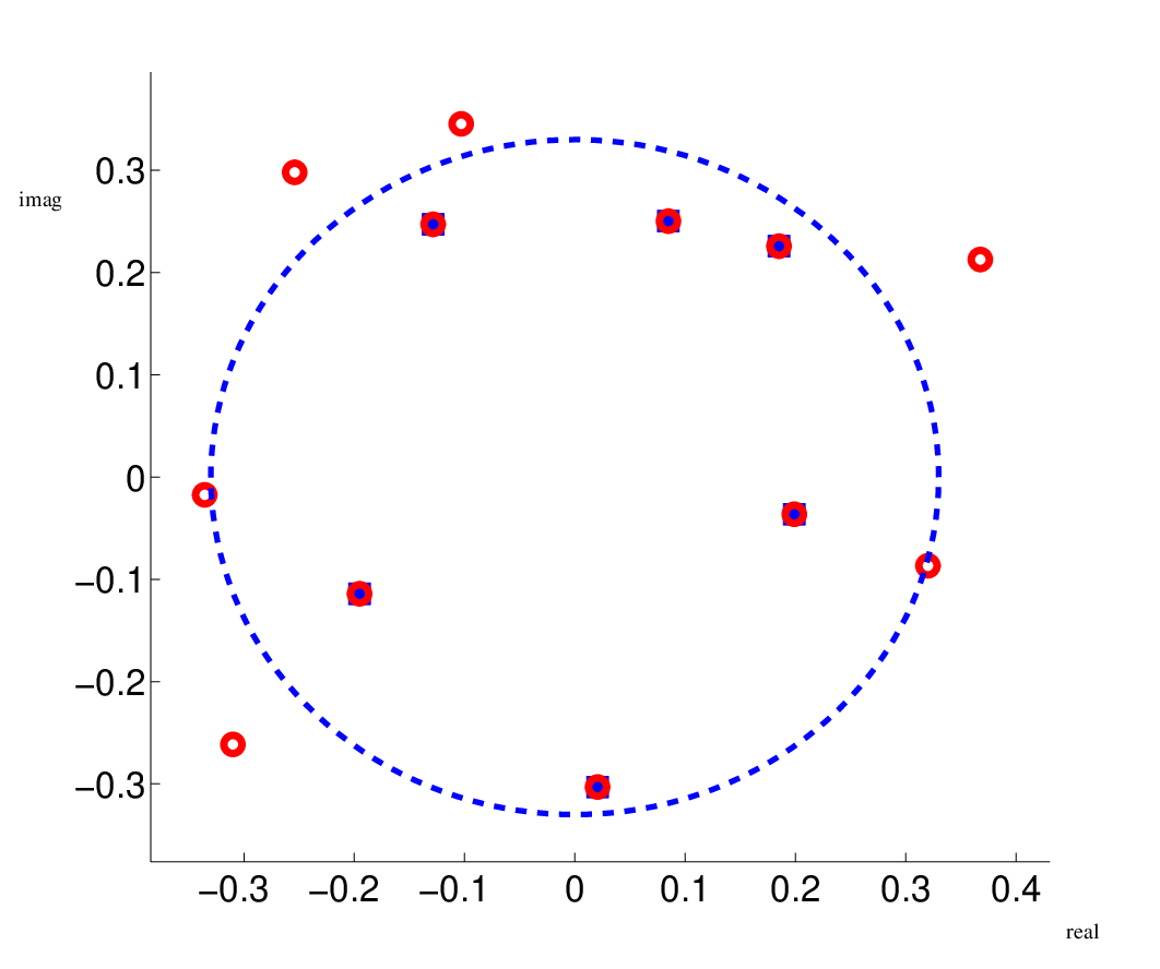
For the next experiment we take random complex entries in (44), a fixed number l=10l=10 of columns, and the same circle as in (45). Again, the 66 eigenvalues inside the circle from polyeig are well approximated by the integral algorithm, see Figure 3 (left).
Refer to caption
Refer to caption
Figure 3: Example 4.10. Eigenvalues from polyeig (open circles) and eigenvalues from the integral algorithm for a random quadratic complex matrix polynomial (left), singular values of integral algorithm with l=10l=10 columns versus the number NN of quadrature nodes for the same example (right).

But this time the singular values do not separate as well as in Figure 2 (left). Two of them decay rather slowly, while two others, due to eigenvalues very close but outside the contour, remain of order one. However, this behavior does not result in spurious eigenvalues. On the contrary, if we keep l=10l=10 for the eigenvalue computation, then this yields the 66 eigenvalues inside and in addition the four eigenvalues lying closest to the contour, but outside. Such a behavior is also suggested by our error analyis in Section 4.1 according to which the principle error term depends on the distance of eigenvalues to the contour, both for eigenvalues inside and outside. Computational experience shows that only very small singular values (≈10−10\approx 10^{-10}) lead to spurious eigenvalues and these can be easily avoided by the residual test in Step 6.

Example 4.11.

This example, taken from [17] and [11], is a finite element discretization of a nonlinear boundary eigenvalue problem

−u′′​(x)=λ​u​(x),0≤x≤1,u⁡(0)=0=u′​(1)+λλ−1​u​(1).-u^{\prime\prime}(x)=\lambda u(x),0\leq x\leq 1,u(0)=0=u^{\prime}(1)+\frac{\lambda}{\lambda-1}u(1).

The matrix function is T⁡(z)=T1+11−z​em​emT−z​T3T(z)=T_{1}+\frac{1}{1-z}e_{m}e_{m}^{T}-zT_{3}, where

T1=m​(2−1−1⋱⋱⋱2−1−11),T3=16​m​(411⋱⋱⋱4112).T_{1}=m\begin{pmatrix}2&-1&&\\ -1&\ddots&\ddots&\\ &\ddots&2&-1\\ &&-1&1\end{pmatrix},\quad T_{3}=\frac{1}{6m}\begin{pmatrix}4&1&&\\ 1&\ddots&\ddots&\\ &\ddots&4&1\\ &&1&2\end{pmatrix}.

We use m=400m=400 and compute five eigenvalues in the interval [2,298][2,298]. Again Figure 4 (left) shows the real eigenvalues in the circle which agree with those from [11]. Note that we avoided the singularity of TT at z=1z=1. The residuals of the computed eigenvectors and eigenvalues decay exponentially as expected, see Figure 4, but not as smooth as in the previous examples.

Refer to caption
Refer to caption
Figure 4: Example 4.11. Eigenvalues from the integral algorithm for the finite element discretization of a nonlinear boundary eigenvalue problem (left), decay of residuals res⁡(λj)=‖T⁡(λj)​(vj)‖\mathrm{res}(\lambda_{j})=||T(\lambda_{j})(v_{j})|| for λ1≈24\lambda_{1}\approx 24 (open circles), λ2≈123\lambda_{2}\approx 123 (filled circles) versus the number NN of quadrature nodes for the same example (right).
Example 4.12.

Consider the quadratic polynomial

T(z)=T0+(z−a)(b−z)T1,a<b∈ℝ,T0,T1∈ℝ15,15,T(z)=T_{0}+(z-a)(b-z)T_{1},\quad a<b\in\mathbb{R},\quad T_{0},T_{1}\in\mathbb{R}^{15,15}, (46)

where T0T_{0} has zeroes in the first column. All other entries of T0,T1T_{0},T_{1} are chosen at random. Then T⁡(z)T(z) has different eigenvalues aa and bb with the same eigenvector e1∈ℝme^{1}\in\mathbb{R}^{m}. This is a critical case since the rank condition (17) is violated. In Figure 5 (left) we show the results of polyeig and of the integral algorithm (with l=5l=5 and the data from (45)). There are three eigenvalues inside the circle. Both eigenvalues a=−0.2a=-0.2 and b=0.1b=0.1 are missed by the integral method, while the third one is found, though at lower accuracy than in the previous examples. Figure 5 shows that only one singular value stays of order one when NN is increased. This example will be reconsidered in Section 5.

Refer to caption
Refer to caption
Figure 5: Example 4.11. Eigenvalues from polyeig (open circles) and eigenvalues from the integral algorithm for a quadratic matrix polynomial with rank defect (left), singular values of integral algorithm with l=5l=5 columns versus the number NN of quadrature nodes for the same example (right).

5 The algorithm for many eigenvalues

In this section we show how the method from Section 3 can be extended to nonlinear eigenvalue problems with more eigenvalues than the dimension of the system, i.e. m<km<k, and to the rank deficient cases, see Remark 3.2 and Example 4.12.

5.1 Construction of algorithm

In case m<km<k condition (17) is always violated and there is no matrix V^\hat{V} satisfying (16). Therefore, we compute more integrals of type (18),(19), namely

Ap=12​π​i​∫Γzp​T​(z)−1​V^​𝑑z∈ℂm,l,p∈ℕ.A_{p}=\frac{1}{2\pi i}\int_{\Gamma}z^{p}T(z)^{-1}\hat{V}dz\in{\mathbb{C}}^{m,l},\quad p\in{\mathbb{N}}.

Here we assume that V^∈ℂm,l\hat{V}\in\mathbb{C}^{m,l} with l≤ml\leq m. In fact, in case k>mk>m we set V^=Im\hat{V}=I_{m} instead of making a random choice.

From Theorem 2.9 we obtain

Ap=V​Λp​WH​V^,p∈ℕ,A_{p}=V\Lambda^{p}W^{H}\hat{V},\;\;p\in{\mathbb{N}}, (47)

where V,W∈ℂm,kV,W\in\mathbb{C}^{m,k} are given by (26) and (28) and Λ\Lambda has the normal form (29).

Now we choose K∈ℕ,K≥1K\in{\mathbb{N}},K\geq 1 and form the K​m×K​lKm\times Kl matrices

B0=(A0⋯AK−1AK−1⋯A2​K−2),B1=(A1⋯AKAK⋯A2​K−1).B_{0}=\begin{pmatrix}A_{0}&\cdots&A_{K-1}\\ \vdots&&\vdots\\ A_{K-1}&\cdots&A_{2K-2}\end{pmatrix},\quad B_{1}=\begin{pmatrix}A_{1}&\cdots&A_{K}\\ \vdots&&\vdots\\ A_{K}&\cdots&A_{2K-1}\end{pmatrix}. (48)

From (47) we find the representations

B0=(VV​ΛK−1)​(WH​V^⋯ΛK−1​WH​V^),B_{0}=\begin{pmatrix}V\\ \vdots\\ V\Lambda^{K-1}\end{pmatrix}\begin{pmatrix}W^{H}\hat{V}&\cdots&\Lambda^{K-1}W^{H}\hat{V}\end{pmatrix}, (49)

and

B1=(VV​ΛK−1)​Λ​(WH​V^⋯ΛK−1​WH​V^).B_{1}=\begin{pmatrix}V\\ \vdots\\ V\Lambda^{K-1}\end{pmatrix}\Lambda\begin{pmatrix}W^{H}\hat{V}&\cdots&\Lambda^{K-1}W^{H}\hat{V}\end{pmatrix}. (50)

We assume that KK has been chosen such that the following rank condition holds

rank​(VV​ΛK−1)=k.\text{rank}\begin{pmatrix}V\\ \vdots\\ V\Lambda^{K-1}\end{pmatrix}=k. (51)

The smallest index having this property is called the minimality index in [11]. In case k>mk>m this can be expected to hold if we choose

(K−1)​m<k≤K​m.(K-1)m<k\leq Km.

In case k≤mk\leq m with rank⁡(V)<k\mathrm{rank}(V)<k (see Remark 3.2(b)) the following lemma shows that (51) holds for KK larger than the sum of the maximal ranks at all eigenvalues.

Lemma 5.1.

Let the assumptions of Corollary 2.8 be satisfied. Then the rank conditon (51) holds with kk as defined in (15) for

K≥∑n=1n⁡(𝒞)max1≤ℓ≤Ln⁡mℓ,n.K\geq\sum_{n=1}^{n(\mathcal{C})}\max_{1\leq\ell\leq L_{n}}m_{\ell,n}.
Proof.

Let Mn=max1≤ℓ≤Ln⁡mℓ,nM_{n}=\max_{1\leq\ell\leq L_{n}}m_{\ell,n} and M=∑n=1n⁡(𝒞)MnM=\sum_{n=1}^{n(\mathcal{C})}M_{n}. Assume that VΛjx=0,j=0,…,M−1V\Lambda^{j}x=0,j=0,\ldots,M-1 for some x∈ℂmx\in\mathbb{C}^{m}. For any n∈{1,…,n⁡(𝒞)}n\in\{1,\ldots,n(\mathcal{C})\} and 0≤β≤Mn−10\leq\beta\leq M_{n}-1 consider the polynomial

Pn,β​(z)=(z−λn)β​∏r=1,r≠nn⁡(𝒞)(z−λr)Mr.P_{n,\beta}(z)=(z-\lambda_{n})^{\beta}\prod_{r=1,r\neq n}^{n(\mathcal{C})}(z-\lambda_{r})^{M_{r}}.

By our assumption 0=V​Pn,β​(Λ)​x0=VP_{n,\beta}(\Lambda)x. We partition according to (29)

V=\displaystyle V= (V1⋯Vn⁡(𝒞)),Vn=(Vn,1⋯Vn,Ln),Vn,ℓ=(v0ℓ,n⋯vmℓ,n−1ℓ,n)\displaystyle\begin{pmatrix}V_{1}&\cdots&V_{n(\mathcal{C})}\end{pmatrix},V_{n}=\begin{pmatrix}V_{n,1}&\cdots&V_{n,L_{n}}\end{pmatrix},V_{n,\ell}=\begin{pmatrix}v^{\ell,n}_{0}&\cdots&v^{\ell,n}_{m_{\ell,n}-1}\end{pmatrix}
x=\displaystyle x= (x1⋯xn⁡(𝒞)),xn=(x1,n⋯xLn,n),xℓ,n=(x0ℓ,n⋯xmℓ,n−1ℓ,n).\displaystyle\begin{pmatrix}x_{1}&\cdots&x_{n(\mathcal{C})}\end{pmatrix},x_{n}=\begin{pmatrix}x_{1,n}&\cdots&x_{L_{n},n}\end{pmatrix},x_{\ell,n}=\begin{pmatrix}x^{\ell,n}_{0}&\cdots&x^{\ell,n}_{m_{\ell,n}-1}\end{pmatrix}.

Using (Jn~−λn~)Mn~=0(J_{\tilde{n}}-\lambda_{\tilde{n}})^{M_{\tilde{n}}}=0 for n~≠n\tilde{n}\neq n we obtain

0=∑ℓ=1LnVn,ℓ​∏n~≠n,mℓ,n−1≥βn⁡(𝒞)(Jn,ℓ−λn~)Mn~​(Jn,ℓ−λn)β​xℓ,n.0=\sum_{\ell=1}^{L_{n}}V_{n,\ell}\prod_{\tilde{n}\neq n,m_{\ell,n}-1\geq\beta}^{n(\mathcal{C})}(J_{n,\ell}-\lambda_{\tilde{n}})^{M_{\tilde{n}}}(J_{n,\ell}-\lambda_{n})^{\beta}x_{\ell,n}. (52)

From this we conclude by induction on β=Mn−1,…,0\beta=M_{n}-1,\ldots,0 that

xνn,ℓ=0,if​β≤ν≤mℓ,n−1.x^{n,\ell}_{\nu}=0,\quad\text{if}\;\beta\leq\nu\leq m_{\ell,n}-1. (53)

For β=Mn−1\beta=M_{n}-1, equation (52) reads

0=∏n~≠nn⁡(𝒞)(λn−λn~)Mn~​∑ℓ=1,mℓ,n=MnLnv0ℓ,n​xmℓ,n−1ℓ,n,0=\prod_{\tilde{n}\neq n}^{n(\mathcal{C})}(\lambda_{n}-\lambda_{\tilde{n}})^{M_{\tilde{n}}}\sum_{\ell=1,m_{\ell,n}=M_{n}}^{L_{n}}v_{0}^{\ell,n}x^{\ell,n}_{m_{\ell,n}-1},

and thus (53) holds for β=Mn\beta=M_{n} by the linear independence of the vectors v0ℓ,nv_{0}^{\ell,n} (cf. Definition 2.5 (iv)). For the induction step we use (52) with β−1\beta-1 instead of β\beta. Together with (53) we find

0=∏n~≠nn⁡(𝒞)(λn−λn~)Mn~​∑ℓ=1,mℓ,n≥βLnv0ℓ,n​xβ−1ℓ,n,0=\prod_{\tilde{n}\neq n}^{n(\mathcal{C})}(\lambda_{n}-\lambda_{\tilde{n}})^{M_{\tilde{n}}}\sum_{\ell=1,m_{\ell,n}\geq\beta}^{L_{n}}v_{0}^{\ell,n}x^{\ell,n}_{\beta-1},

which shows that (53) holds for β−1\beta-1. Thus we have shown x=0x=0 and this finishes the proof. ∎

The computational procedure is now a straightforward generalization of Section 3.1. First compute B0,B1∈ℂK​m,K​lB_{0},B_{1}\in\mathbb{C}^{Km,Kl} from (48). In addition to (51), assume

rank​(WH​V^⋯ΛK−1​WH​V^)=k.\mathrm{rank}\begin{pmatrix}W^{H}\hat{V}&\cdots&\Lambda^{K-1}W^{H}\hat{V}\end{pmatrix}=k. (54)

Let us abbreviate

V[K]=(VV​ΛK−1)∈ℂK​m,k,W[K]H=(WH​V^⋯ΛK−1​WH​V^)∈ℂk,K​l.V_{[K]}=\begin{pmatrix}V\\ \vdots\\ V\Lambda^{K-1}\end{pmatrix}\in\mathbb{C}^{Km,k},\quad W_{[K]}^{H}=\begin{pmatrix}W^{H}\hat{V}&\cdots&\Lambda^{K-1}W^{H}\hat{V}\end{pmatrix}\in\mathbb{C}^{k,Kl}.

Compute the SVD

V[K]​W[K]H=B0=V0​Σ0​W0H,V_{[K]}W_{[K]}^{H}=B_{0}=V_{0}\Sigma_{0}W_{0}^{H},

where V0∈ℂK​m,k,V0H​V0=IkV_{0}\in\mathbb{C}^{Km,k},V_{0}^{H}V_{0}=I_{k}, Σ0=diag​(σ1,…,σk)∈ℂk,k\Sigma_{0}=\text{diag}(\sigma_{1},\ldots,\sigma_{k})\in\mathbb{C}^{k,k}, and W0∈ℂK​l,kW_{0}\in\mathbb{C}^{Kl,k}, W0H​W0=IkW_{0}^{H}W_{0}=I_{k}. From the rank conditions (51),(54),

σ1≥…​σk>0=σk+1=…=σK​l.\sigma_{1}\geq\ldots\sigma_{k}>0=\sigma_{k+1}=\ldots=\sigma_{Kl}.

The rank condition (51) also implies

R⁡(B0)=R⁡(V[K])=R⁡(V0).R(B_{0})=R(V_{[K]})=R(V_{0}).

Thus the matrix S=V0H​V[K]∈ℂk,kS=V_{0}^{H}V_{[K]}\in\mathbb{C}^{k,k} is nonsingular and satisfies

V[K]=V0​S.V_{[K]}=V_{0}S. (55)

With (49), (55) we find

W[K]H=S−1​Σ0​W0H,W_{[K]}^{H}=S^{-1}\Sigma_{0}W_{0}^{H},

and then from (50)

B1=V[K]​Λ​W[K]H=V0​S​Λ​S−1​Σ0​W0H.B_{1}=V_{[K]}\Lambda W_{[K]}^{H}=V_{0}S\Lambda S^{-1}\Sigma_{0}W_{0}^{H}.

Finally, this leads to

D:=V0H​B1​W0​Σ0−1=S​Λ​S−1.D:=V_{0}^{H}B_{1}W_{0}\Sigma_{0}^{-1}=S\Lambda S^{-1}. (56)

Therefore, the analog of Theorem 3.3 is

Theorem 5.2.

Suppose that T∈H⁡(Ω,ℂm,m)T\in H(\Omega,\mathbb{C}^{m,m}) has no eigenvalues on the contour Γ\Gamma in Ω\Omega and pairwise distinct eigenvalues λn,n=1,…,n⁡(Γ)\lambda_{n},n=1,\ldots,n(\Gamma) inside Γ\Gamma with partial multiplicities m1,n≥…≥mLn,n,n=1,…,n(Γ)m_{1,n}\geq\ldots\geq m_{L_{n},n},n=1,\ldots,n(\Gamma). Assume that the rank conditions (51),(54) are satisfied with kk given by (15). Then the matrix D∈ℂk,kD\in\mathbb{C}^{k,k} from (56) has Jordan normal form (29) with the same eigenvalues λn\lambda_{n} and partial multiplicities mℓ,nm_{\ell,n} (ℓ=1,…,Ln,n=1,…,n⁡(Γ)\ell=1,\ldots,L_{n},n=1,\ldots,n(\Gamma)). Suitable CSGEs for TT can be obtained from corresponding CSGEs sjℓ,ns_{j}^{\ell,n} for DD via

vjℓ,n=V0[1]​sjℓ,n,0≤j≤mℓ,n−1,1≤ℓ≤Ln,1≤n≤n⁡(Γ),v_{j}^{\ell,n}=V_{0}^{[1]}s_{j}^{\ell,n},\quad 0\leq j\leq m_{\ell,n}-1,1\leq\ell\leq L_{n},1\leq n\leq n(\Gamma),

where V0[1]V_{0}^{[1]} is the upper m×km\times k block in

V0=(V0[1]V0[K]).V_{0}=\begin{pmatrix}V_{0}^{[1]}\\ \vdots\\ V_{0}^{[K]}\end{pmatrix}. (57)
Remark 5.3.

In a sense this generalization is similar to linearizing a polynomial eigenvalue problem by increasing the dimension. Note, however, that this only becomes necessary if there are too many eigenvalues inside the contour, or if rank defects occur that are not present in linear eigenvalue problems.

The generalization of the algorithm from Section 3.3 is the following.

Integral algorithm 2

Step 1: Choose numbers l≤ml\leq m, K≥1K\geq 1 and a matrix V^∈ℂm,l\hat{V}\in\mathbb{C}^{m,l} at random. If more than mm eigenvalues are expected inside Γ\Gamma, let l=m,V^=Iml=m,\hat{V}=I_{m}.

Step 2: Compute

Ap,N=1i​N∑j=0N−1T(φ(tj))−1V^φ(tj)pφ′(tj),p=0,…,2K−1,A_{p,N}=\frac{1}{iN}\sum_{j=0}^{N-1}T(\varphi(t_{j}))^{-1}\hat{V}\varphi(t_{j})^{p}\varphi^{\prime}(t_{j}),\quad p=0,\ldots,2K-1,

and form B0,NB_{0,N},B1,NB_{1,N} as in (48).

Step 3: Compute the SVD B0,N=V​Σ​WHB_{0,N}=V\Sigma W^{H}, where
V∈ℂK​m,K​lV\in\mathbb{C}^{Km,Kl}, W∈ℂK​l,K​lW\in\mathbb{C}^{Kl,Kl}, VH​V=WH​W=IK​lV^{H}V=W^{H}W=I_{Kl}, Σ=diag⁡(σ1,σ2,…,σK​l)\Sigma=\mathrm{diag}(\sigma_{1},\sigma_{2},\ldots,\sigma_{Kl}).

Step 4: Perform a rank test for Σ\Sigma, i.e. find 0<k≤K​l0<k\leq Kl such that
σ1≥…≥σk>σk+1≈…≈σK​l≈0\sigma_{1}\geq\ldots\geq\sigma_{k}>\sigma_{k+1}\approx\ldots\approx\sigma_{Kl}\approx 0.
If k=K​lk=Kl then increase ll or KK and go to Step 1.
Else let V0=V(1:Km,1:k),W0=W(1:Kl,1:k)V_{0}=V(1:Km,1:k),W_{0}=W(1:Kl,1:k) and
Σ0=diag⁡(σ1,σ2,…,σk)\Sigma_{0}=\mathrm{diag}(\sigma_{1},\sigma_{2},\ldots,\sigma_{k}).

Step 5: Compute D=V0H​B1,N​W0​Σ0−1∈ℂk,kD=V_{0}^{H}B_{1,N}W_{0}\Sigma_{0}^{-1}\in\mathbb{C}^{k,k}.

Step 6: Solve the eigenvalue problem for DD
D​S=S​ΛDS=S\Lambda, S=(s1​…​sk),Λ=diag⁡(λ1,…,λk)S=(s_{1}\ldots s_{k}),\Lambda=\mathrm{diag}(\lambda_{1},\ldots,\lambda_{k}).
If ‖T⁡(λj)​vj‖||T(\lambda_{j})v_{j}|| is small and λj∈int⁡(Γ)\lambda_{j}\in\mathrm{int}(\Gamma) accept vj=V0[1]​sjv_{j}=V_{0}^{[1]}s_{j} (with V0[1]V_{0}^{[1]} from (57)) as eigenvector and λj\lambda_{j} as eigenvalue.

5.2 Numerical Examples

Example 5.4.

We apply the integral algorithm 2 to the rank deficient example (46), where K=2,l=3K=2,l=3 and the contour is the circle from (45). Now the eigenvalues a=−0.2a=-0.2 and b=1b=1 are reproduced correctly (see Figure 6(left)), and three singular values survive as expected (Figure 6 (right)).

Refer to caption
Refer to caption
Figure 6: Example 5.4. Eigenvalues from polyeig (open circles) and eigenvalues from the integral algorithm 2 (K=2K=2, filled boxes) for a quadratic matrix polynomial with rank defect (left), singular values of integral algorithm 22 with l=3l=3 columns versus the number NN of quadrature nodes for the same example (right).
Refer to caption
Refer to caption
Figure 7: Example 5.5.Eigenvalues of the characteric equation (58) inside a circle of radius 66 and with center −1-1, computed with the integral algorithm 2 with K=3,l=2K=3,l=2. (left), residuals ‖T⁡(λj)​vj‖||T(\lambda_{j})v_{j}|| for λ1≈−0.6+2.71​i\lambda_{1}\approx-0.6+2.71i, λ2≈−2.27+5.07​i\lambda_{2}\approx-2.27+5.07i versus the number NN of quadrature nodes for the same example (right).
Example 5.5.

Consider the characteristic equation of a delay system x˙=T0​x​(t)+T1​x​(t−τ)\dot{x}=T_{0}x(t)+T_{1}x(t-\tau) from [16, Sec.2.4.2],[11], given by

T⁡(z)=z​I−T0−T1​e−z​τ,T0=(−512−6),T1=(−214−1).T(z)=zI-T_{0}-T_{1}e^{-z\tau},\quad T_{0}=\begin{pmatrix}-5&1\\ 2&-6\end{pmatrix},\quad T_{1}=\begin{pmatrix}-2&1\\ 4&-1\end{pmatrix}. (58)

In case τ=1\tau=1 there are more than two eigenvalues inside the circle φ⁡(t)=z0+R​ei​t,μ=−1,R=6\varphi(t)=z_{0}+Re^{it},\mu=-1,R=6 . We set l=2,V^=I2l=2,\hat{V}=I_{2} and K=3K=3 for the integral algorithm 2 and obtain with N=150N=150 five eigenvalues inside the circle, (see Figure 7(left)), which coincide with the computed ones in [11]. Much smaller values than N=150N=150 give sufficient accuracy, since there is a good separation of singular values and a fast decay of residuals, see Figure 7(right).

References

  • [1] T. Betcke, N. J. Higham, V. Mehrmann, C. Schröder, and F. Tisseur. NLEVP: A collection of nonlinear eigenvalue problems. Technical Report 2008.40, MIMS, University of Manchester, Apr. 2008. www.mims.manchester.ac.uk/research/numerical-analysis/nlevp.html.
  • [2] T. Betcke and H. Voss. A Jacobi-Davidson type projection method for nonlinear eigenvalue problems. Future Gener. Comput. Syst., 20:363–372, 2004.
  • [3] P. J. Davis. On the numerical integration of periodic analytic functions. In On numerical approximation. Proceedings of a Symposium, Madison, April 21-23, 1958, Edited by R. E. Langer. Publication no. 1 of the Mathematics Research Center, U.S. Army, the University of Wisconsin, pages 45–59. The University of Wisconsin Press, Madison, 1959.
  • [4] P. J. Davis and P. Rabinowitz. Methods of numerical integration. Dover Publications Inc., Mineola, NY, 2007. Corrected reprint of the second (1984) edition.
  • [5] I. C. Gohberg and E. I. Sigal. An operator generalization of the logarithmic residue theorem and Rouché’s theorem. Mat. Sb. (N.S.), 84(126):607–629, 1971.
  • [6] R. E. Greene and S. G. Krantz. Function theory of one complex variable, volume 40 of Graduate Studies in Mathematics. American Mathematical Society, Providence, RI, third edition, 2006.
  • [7] N. Hale, N. J. Higham, and L. Trefethen. Computing Aα{A}^{\alpha}, log⁡(A)\log({A}), and related matrix functions by contour integrals. SIAM J. Numer. Anal., 46:2505–2523, 2008.
  • [8] N. J. Higham. Functions of Matrices. SIAM, 2008.
  • [9] M. V. Keldysh. On the characteristic values and characteristic functions of certain classes of non-self-adjoint equations. Doklady Akad. Nauk SSSR (N.S.), 77:11–14, 1951.
  • [10] M. V. Keldysh. The completeness of eigenfunctions of certain classes of nonselfadjoint linear operators. Uspehi Mat. Nauk, 26(4(160)):15–41, 1971.
  • [11] D. Kressner. A block Newton method for nonlinear eigenvalue problems. Numer. Math., 114:355–372, 2009.
  • [12] A. S. Markus and E. I. Sigal. The multiplicity of the characteristic number of an analytic operator function. Mat. Issled., 5(3(17)):129–147, 1970.
  • [13] V. Mehrmann and H. Voss. Nonlinear eigenvalue problems: a challenge for modern eigenvalue methods. GAMM Mitteilungen, 27, 2004.
  • [14] R. Mennicken and M. Möller. Root functions, eigenvectors, associated vectors and the inverse of a holomorphic operator function. Arch. Math. (Basel), 42(5):455–463, 1984.
  • [15] R. Mennicken and M. Möller. Non-self-adjoint boundary eigenvalue problems, volume 192 of North-Holland Mathematics Studies. North-Holland Publishing Co., Amsterdam, 2003.
  • [16] W. Michiels and S.-I. Niculescu. Stability and Stabilization of Time-delay Systems, volume 12 of Advances in Design and Control. Society for Industrial and Applied Mathematics (SIAM), 2007.
  • [17] S. Solovev. Preconditioned iterative methods for a class of nonlinear eigenvalue problems. Linear Algebra Appl., 415:210–229, 2006.
  • [18] G. Stewart and J. G. Sun. Matrix Perturbation Theory. Academic Press Inc., Boston, MA, 1990.
  • [19] V. P. Trofimov. The root subspaces of operators that depend analytically on a parameter. Mat. Issled., 3(vyp. 3 (9)):117–125, 1968.
  • [20] H. Voss. A maxmin principle for nonlinear eigenvalue problems with application to a rational spectral problem in fluid-solid vibration. Appl. Math, 48:607–622, 2003.
  • [21] H. Voss. An Arnoldi method for nonlinear eigenvalue problems. BIT, 44:387–401, 2004.
  • [22] H. Voss. A Jacobi-Davidson method for nonlinear and nonsymmetric eigenvalue problems. Comput. Struct., 85:1284–1292, 2007.
  • [23] H. Voss and B. Werner. A minmax principle for nonlinear eigenvalue problems with applications to nonoverdamped systems. Math. Methods Appl. Sci., 4:415–424, 1982.