Braid Matrices and Quantum Gates for Ising Anyons Topological Quantum Computation
Abstract
We study various aspects of the topological quantum computation scheme based on the non-Abelian anyons corresponding to fractional quantum hall effect states at filling fraction 5/2 using the Temperley-Lieb recoupling theory. Unitary braiding matrices are obtained by a normalization of the degenerate ground states of a system of anyons, which is equivalent to a modification of the definition of the 3-vertices in the Temperley-Lieb recoupling theory as proposed by Kauffman and Lomonaco. With the braid matrices available, we discuss the problems of encoding of qubit states and construction of quantum gates from the elementary braiding operation matrices for the Ising anyons model. In the encoding scheme where 2 qubits are represented by 8 Ising anyons, we give an alternative proof of the no-entanglement theorem given by Bravyi and compare it to the case of Fibonacci anyons model. In the encoding scheme where 2 qubits are represented by 6 Ising anyons, we construct a set of quantum gates which is equivalent to the construction of Georgiev.
I Introduction
Quantum computers are expected to be able to perform calculations which are impossible for classical computers, due to quantum entanglement and quantum parallelism [1]. Unfortunately, quantum computers seem to be extremely difficult to build because of the unavoidable noise and decoherence caused by the coupling of the qubits and the ambient environment. It is a daunting task to construct a quantum computer that has a large number of qubits and has a low error rate. However, there is a promising approach, called topological quantum computation (TQC) [2, 3, 4, 5, 6, 7, 8, 9, 10, 11, 12, 13], proposing to encode the qubit information into a topological quantum field. Kitaev [2] proposed that a system of anyons can be considered to be a quantum computer. Unitary matrices are related to moving the anyons around each other. Measurements are performed by joining anyons in pairs and observing the result of fusion. Interference experiments [14, 15, 16, 17, 18, 19] are also proposed to initialize and read out quantum states. The computation is fault-tolerant by the topological nature of the system.
Different from fermions and bosons, which are the totally antisymmetric and the symmetric representations of the permutation group , anyons carry fractional charges and have fractional statistics [20, 21] which result in nontrivial phases (for Abelian anyons) or matrices (for non-Abelian anyons) for permutations. In fact, the underlying symmetry of the system of anyons is the braid group . Abelian anyons correspond to one-dimensional representations of and the quantum gates one can construct from them are very limited [22]. Non-Abelian anyons, on the contrary, are much more useful to TQC, since the braiding of non-Abelian anyons induces non-commuting (non-Abelian) representations of , from which one can construct various quantum gates.
Physically, anyons are collective excitations in some condensed matter systems, such as the fractional quantum hall effect (FQHE) states of two dimensional electron liquids. For example, the effective theories of FQHE states with filling levels , and correspond to Abelian anyons, non-Abelian Moore-Read [23] and Read-Rezayi [24] anyons respectively. Mathematically, properties of anyons can be described by Chern-Simons effective field theories [25] and parafermion conformal field theories (CFT) [26], the and cases corresponding to the and the FQHE states respectively.
The Chern-Simons theory is a topological quantum field theory [25] which has a deep relationship to knot invariants, Jones Polynomial [27] especially. Kauffman and Lomonaco [28, 29] studied unitary representations of braid groups in terms of -deformed spin networks, or Temperley-Lieb recoupling theory [30].
It is one of our purpose to apply the method of Kauffman and Lomonaco to calculate explicitly the elementary braiding operation (EBO) matrices which govern the exchanges of Ising anyons, the first non-Abelian anyons model proposed by Moore and Read [23] by constructing a wave function (the Pfaffian state) for the FQHE state corresponding to the Chern-Simons theory. Direct experimental observation of fractional electron charge [31, 32] at the FQHE state gives some evidences in support of the non-Abelian nature of this state. There are many works concerning the braiding properties of the Ising anyons using CFT method [33, 34] or quantum group method [35]. Nayak and Wilczek [33] suggested that the Pfaffian wave functions of ( even) Ising anyons form a dimensional spinor irreducible representation of the rotation group , to which a rigorous treatment is given by Georgiev recently [34]. Quantum group approach [35] also gives equivalent results. As we will see, the EBO matrices for the Ising anyons can be elegantly derived by using the Temperley-Lieb recoupling theory.
One of the attractive properties of the Ising anyons TQC model is that the excitation gap at the corresponding filling fraction is the highest one among all non-Abelian FQHE states, resulting in a very low (or even lower) error rate of [36, 37, 38]. Although this Ising anyons model is not universal [4, 5, 6] for TQC, i.e., the braid group representations are not dense in unitary groups, it receives extensive attention in the past few years [38, 39, 40, 41, 42, 43, 44, 45]. In fact, it is proved by Bravyi [39] that no entangled states in the computational space can be obtained purely topologically and the Ising anyons TQC model is classically simulatable. We show that the same conclusion can be obtained from the Temperley-Lieb recoupling theory approach.
We should stress that this no-entanglement theorem does not mean that there is no entanglement between Ising anyons at all. This rule only applies to the qubit encoding scheme (which is consistent with the quantum circuit model) where each qubit is encoded in 4 Ising anyons. Entangled quantum gates, such as controlled-Z and controlled-NOT (CNOT), can be realized purely by braiding 6 Ising anyons with definite topological charge (quantum spin). Using the EBO matrices obtained in this paper, we construct a set of useful 1-qubit and 2-qubit quantum gates, which is not the same as, but equivalent to the construction by Georgiev [41, 42].
The outline of the remainder of this paper is as follows. Section 2 reviews the general models of non-Abelian anyons for TQC and the formalism of the Temperley-Lieb recoupling theory needed later. Unitary representations of the braid group in the Hilbert space of the degenerate ground states of non-Abelian anyons are obtained by a physical argument which requires that the fusion paths of the anyons form an orthonomal basis of the Hilbert space. In section 3, we derive the EBO matrices of the Ising anyons model. In section 4, we study some aspects of Ising anyons TQC using the results of section 3. Conclusions and discussions are presented in Section 5.
II Temperley-Lieb recoupling theory and unitary representations of braid groups
In this section, we first review the definition of the quantum states of a system of anyons and the Temperley-Lieb recoupling theory [30] and then discuss the method to produce unitary representations of braid groups.
II.1 Models of non-Abelian anyons for TQC
A model of non-Abelian anyons consists of the following three elements [11]: a list of particle types, the fusion rules, and the braiding rules. In the formalism of Chern-Simons theory, anyons are quasi-particles having half-integer -spins (spins for short) as their quantum numbers. The fusion rules of these particles are truncated versions of the rules of addition of ordinary angular momenta,
| (1) |
When a number of non-Abelian anyons with definite spins fuse consecutively into a single anyon with some spin, the sequences of the intermediate spins of the fusion paths represent different quantum states of the Hilbert space.
Anyons commonly appear as collective excitations in 2 dimensional systems. When they move, their world lines propagate in a 3 dimensional space-time. Thus the exchange of a pair of anyons corresponds to the braiding of their world-lines. (We will call the braiding of the world-lines of anyons shortly as the braiding of anyons, but it is important to keep in mind what it means actually.) In TQC, we perform quantum computations by braiding anyons to realize certain quantum gates. Any braiding can be expressed as a sequence of EBOs whose representations in the above Hilbert space are the EBO matrices we want to find. The essential task of deriving the EBO matrices is the determination of the so called R-matrix and F-matrix introduced first in the context of CFT [49]. The former is the unitary matrix inducing the exchange of neighboring anyons with definite total spin, and the latter accounts for the associativity of fusions of anyons. In the next subsection, we will give their diagrammatic definitions in terms of the Temperley-Lieb recoupling theory.
II.2 Temperley-Lieb recoupling theory
Temperley-Lieb recoupling theory [30] is based on the Kauffman bracket polynomial model for the Jones polynomial at roots of unity and the tangle-theoretic Temperley-Lieb algebra.
II.2.1 Braid group and Temperley-Lieb algebra
The Artin braid group can be presented as a set of generators that obey the following relations,
| (2) |
The Temperley-Lieb algebra can be presented similarly as a set of generators , whose representations are related to the representations of by
| (3) |
where the Kauffman variable is taken to be for Jones polynomial at -th roots of unity such that the quantum dimension of the spin 1/2 anyon is .
II.2.2 R-matrix and F-matrix

The basic object of the Temperley-Lieb recoupling theory is the Jones-Wenzl projector [30]. The left graph in Fig. 1 shows the Jones-Wenzl projector constructed on the basis of the Kauffman bracket polynomial expansion. The -strand projector corresponds to the world line of an anyon with spin . The middle graph in Fig. 1 shows the 3-vertex constructed from the projectors which corresponds to the interaction (fusing or splitting) of 3 anyons with spins , , and . The right graph in Fig. 1 is a simplified notation for the 3-vertex. Note that the -admissible conditions [30] for the 3-vertex,
| (4) |
say exactly the same thing as the fusion rules Eq. (1) do due to the relation between Chern-Simon theory at level and Jones polynomial at -th roots of unity [25] and the fact that the projector with label represents the world line of an anyon with spin . Various spin networks can be constructed from Jones-Wenzl projectors and 3-vertices. See Fig. 2.


As the world lines of anyons and their fusions being identified with projectors and 3-vertices, we now consider the braiding properties of anyons in the context of the Temperley-Lieb recoupling theory. Fig. 3 shows the braiding of two anyons with spins and fusing into a spin anyon. Since this operation dose not change the total spin of the two fusing anyons, the corresponding matrix, the R-matrix is diagonal in the underlying Hilbert space. The matrix element is given by the following formula [30],
| (5) |


Not all braids are of this case, in which the two braiding anyons fuse into a single anyon. To see this, it is sufficient to consider the case of 4 anyons with total spin 0, which is equivalent to 3 anyons fusing into the 4-th anyon. This is shown in Fig. 4.
The braiding of and in Fig. 5 can not be accomplished via a single R-matrix and is realized only by a combination of the R-matrix and the F-matrix. Fig. 6. shows the definition [30] of the matrix element of the F-matrix as well as the formula to calculate it in terms of the delta net , the theta net , and the tetrahedron net ,
| (6) |

II.3 Unitary representations of Artin braid groups

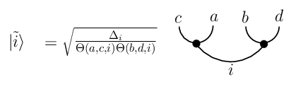
However, the F-matrix defined above in the Temperley-Lieb recoupling theory is not unitary, resulting in a non-unitary representation of the braid group. Unitary (in fact real and orthogonal) F-matrix, and hence unitary representation of can be obtained by a redefinition for the basis states in the Hilbert space of the anyons. The guideline of the following argument is the requirement that the fusion paths should represent an orthonormal basis of the Hilbert space of the degenerate ground states of a system of anyons.
We need only to consider the orthonormal problem of the states of four anyons fusing into the vacuum. The definition of the state and the calculation of the inner product of the two states and are shown in Fig. 7. We see that the orthogonal property is already satisfied (), but the state vectors are not normalized (). It follows that an orthonormal basis () of the Hilbert space is obtained by normalizing each of the states, as depicted in Fig. 8. In the orthonormal basis , the new F-matrix can be derived to be
| (7) |
This new F-matrix is real and orthogonal (hence unitary), as we will see in explicit calculations latter. We note that Kauffman and Lomonaco [28] obtained the unitary F-matrix by multiplying each 3-vertex with the following factor,
| (8) |
One can check that this modification to 3-vertices results in the same F-matrix given by Eq. (7).

III EBO matrices for Ising anyons
In this section, we apply the results of section 2 to obtain explicitly the representations of the generators of the braid group governing the exchanges of Ising anyons. Our presentation follows closely to Kauffman and Lomonaco [28, 29].
For the Ising anyons model, the Kauffman variable is , and the quantum dimension of the spin 1/2 Ising anyons is . The allowed spins of anyons in this model are 0, 1/2 and 1 and the fusion rules for these anyons can be deduced from Eq. (1) to be,
| (9) |
The dimension of the Hilbert space of spin 1/2 Ising anyons with total spin 0 is , approaching in the limit . According to the above fusion rules, the fusion diagram of ( must be odd) Ising anyons with total spin 0 takes the form as shown in Fig. 9 11 1 For later convenience, we make a change of notation. We will label anyons by their spins other than the numbers of strands of the corresponding Jones-Wenzl projectors, which is conventional in the physical literature..
We now calculate the unitary representation of for the braiding of the Ising anyons. We denote the elementary braiding operation (EBO) of the first and the second Ising anyons as , the EBO of the second and the third Ising anyons as , . The corresponding EBO matrices are denoted by where .
The first EBO matrix is easy to calculate. It depends only on the label . In the basis , is simply given by the following R-matrix,
| (10) |
which corresponds to the following Temperley-Leib generator,
| (11) |
To calculate , we need to calculate the following F-matrix in the same basis as above (using Eq. (7) and the formulae in the appendix),
| (12) |
corresponding to the following Temperley-Leib generator,
| (13) |
where .
Now consider the case of . When either or or both of them equal to 0, the situation is similar to the case of where only R-matrix elements are needed to be calculated. The case in which both and are 1 deserves special consideration. The EBO does not change the value of when both and are 1, and the matrix element of in this case is found to be the same as in the case where both and are 0 by doing some graphic calculations.
The other EBO matrices can be calculated in the same way. By choosing the basis of the Ising anyons with total spin 0 ( odd) as where equals to 0, 1/2, or 1 such that the fusion rules are met at each fusion vertex along the whole fusion path, as shown in Fig. 9, we can find a representation of the Temperley-Lieb algebra . For the first and the last generators of , we have,
| (14) |
For and , we have,
| (15) |
For the middle ones, we have,
| (16) |
IV Construct quantum gates from the EBO matrices for the Ising anyons model
After obtaining the EBO matrices of the Ising anyons model, we study in this section some aspects of Ising anyons TQC.
The qubit encoding scheme which is consistent to the quantum circuit model is to use each group of 4 Ising anyons with total spin 0 for each qubit such that an -qubit system uses Ising anyons. This is the encoding scheme used by Bravyi [39] who proved a no-entanglement theorem which states that entangled 2-qubit states can never be prepared by pure topological braiding operations. The proof by Bravyi uses the stabilizer constrains and the no-leakage error conditions. In the following, we give a graphical demonstration of this result from the Temperley-Lieb recoupling approach.


In this qubit encoding scheme, 2-qubit states are encoded in 8 Ising anyons, 4 Ising anyons for each qubit. See Fig. 10. The two groups of EBOs and apply completely within the first and the second qubits respectively and can not generate entanglement between the two qubits. Since depends on and , depends on and , and can change from 0 to a superposition of 0 and 1, it is possible to create an entangled state by a sequence of these EBOs, such as . However, it is impossible to avoid leakage errors by braiding this way. To see this, it is convenient to change the fusion paths in Fig. 10 to another basis as shown in Fig. 11, where the total spin of the 2-qubit system can be either 0 or 1. The EBO sequence in Fig. 10 is equivalent to the single EBO in Fig. 11. Since the braid matrices of in Fig. 11 for the two sectors (total spin 0 and 1) are not equivalent, and entanglement can not be created without using in Fig. 11, leakage error from the computational space (labeled by and in both Fig. 10 and Fig. 11) to the uncomputational space (labeled by in Fig. 10 and in Fig. 11) is unavoidable.
It is instructive to compare the above situation with the case of the Fibonacci anyons [11] model which is universal for TQC [4, 5, 6]. See Fig. 10 too. For Fibonacci anyons, each intermediate spin can be either 0 or 1 (as long as no two 0s appear consecutively) and entangled states can be generated by braiding the 8 Fibonacci anyons. Bonesteel et al [46, 47, 48] constructed some entangled 2-qubit gates such as the controlled- gate by weaving two Fibonacci anyons ( and ) from the control qubit into the target qubit which approximates the identity matrix, followed by a braiding within the target qubit which approximates the gate, and then weaving them back to their original positions. The controlling operation is realized by virtue of the fact that the whole braiding does nothing when the total spin of and is 0 and acts as the gate on the target qubit when the total spin of and is 1. The nonuniversality of the Ising anyons model prevents us from realizing entangled gate in this way.

We note that the no-entanglement theorem only applies to the above qubit encoding scheme where 2 qubits are represented by 8 Ising anyons. Entangled quantum gates can be constructed in a different qubit encoding scheme, as studied by Georgiev [41, 42]. In this scheme, 1-qubit and 2-qubit states are encoded in 4 and 6 Ising anyons with total spin 0 respectively.
Consider 1-qubit gates first. Taking the basis of the Hilbert space to be (see Fig. 9) , the two dimensional EBO matrices of for four Ising anyons are found to be
| (17) |
| (18) |
One can construct the Hadamard gate , the phase gate , and the three Pauli gates , , and using the two dimensional EBO matrices given above ( means equal up to an unimportant global phase),
| (19) |
| (20) |
| (21) |
| (22) |
| (23) |
Fig. 12 shows the encoding of the 1-qubit states as well as the Hadamard gate constructed by three braids.
However, it fails to construct the gate,
| (24) |
reflecting the fact that the Ising anyons model is not universal for quantum computation. To remedy this, we have to supplement braiding with some non-topological operations [39, 40].
Now consider the 2-qubit case. Taking the basis of the Hilbert space to be (see Fig. 9) , , , , the four dimensional EBO matrices of for 6 Ising anyons with total spin 0 read
| (25) |
| (26) |
| (27) |
| (28) |
| (29) |
From the four dimensional EBO matrices given above, one can construct useful 2-qubit quantum gates, such as CNOT (up to an unimportant global phase),
| (30) |
and controlled- ,
| (31) |

Fig. 13 shows the encoding of the 2-qubit states as well as the braiding diagram of CNOT. Note that the braid sequences for CNOT and controlled- are not unique, which is a consequence of the Artin relations Eq. (2) for the generators of the braid group. Our constructions are different from, but equivalent to the ones given by Georgiev [41, 42].
Note that the 4 dimensional Hilbert space of 6 Ising anyons with total spin 0 is a subspace of the 8 dimensional space of 8 Ising anyons. The other subspace, which is also 4 dimensional, corresponds to 6 anyons with total spin 1. See Fig. 11. Using the method in section 3, we can also find the EBO matrices for the spin 1 sector. It turns out that the EBO matrices , , , and in the spin 1 sector take the same form as in the spin 0 sector, but has a different form, . Therefore, entangled 2-qubit quantum gates will have different braid sequences in the spin 1 sector. For example, one possible braid sequence in the spin 1 sector for CNOT is , which is not topologically equivalent to the one given in Eq. (30). Despite of the non-equivalence of the braid sequences for a given quantum gate in these two sectors, the computational power of the two sectors are equivalent [44].
V conclusion and discussion
As demonstrated in previous sections, the Temperley-Lieb recoupling theory provides a natural language for describing the braiding properties of non-Abelian anyons. We have applied this theory to derive the EBO matrices of the Ising anyons model. We paid a special attention to the normalization of the degenerate ground states corresponding to the fusion paths of the anyons. This normalization results in the correct unitary F-matrices and is equivalent to the redefinition of the 3-vertices proposed by Kauffman and Lomonaco [28].
One important feature for the construction of the two-qubit gates is that we can not construct them without the use of , the EBO acting between the two qubits. This is because that the EBOs and act only on the first qubit and and act only on the second qubit. Indeed, the first two and the last two EBO matrices can be expressed as a tensor product of two matrices, and the middle EBO matrix can not, reflecting the (topological) entanglement of the 2 qubits. This entanglement is crucial for the construction of the 2-qubit entangled gates. However, to get this entanglement, we need to project the representation to either the spin 0 or the spin 1 representations. Alternatively, entangled quantum gates can be constructed by parity measurement as well as braiding operations [39, 43].
The construction of the 2-qubit gates in each sector can be easily achieved by brute force search, since the braid lengths of controlled- and CNOT are very short (3 and 7 respectively). However, there is a more heuristic approach, namely, the genetic algorithm (GA) approach. A possible braid sequence for the CNOT gate can be found within a minute using GA, while it takes a much longer time using the brute force approach. The superiority of GA over brute force search is not significant for Ising anyons TQC, but we expect that there is a potential application of GA to Fibonacci anyons topological quantum compiling [46, 47, 48].
Acknowledgements
We thank Jens Fjelstad and Ben Goertzel for numerous discussions. We also thank the referees of EPJB who pointed out a mistake of our original manuscript and helped improve this paper a lot. Z. Fan is supported by National Natural Science Foundation of China under grant numbers 10535010, 10675090, 10775068, and 10735010.
Appendix A Formulae for evaluating the spin-nets
In this appendix, we present the formulae for the evaluations of the -net, the -net, and the tetrahedral net [30].
The -net evaluation is
| (32) |
where is the -deformed integer defined as . The -net evaluation is
| (33) |
where the -deformed fractional is defined as , and the integers , , and are determined by the relations , , and . The bracket evaluation of the tetrahedral net is
| (34) |
where and are given by , , , , , , and .
References
- [1] M. A. Nielsen, and I. L. Chuang, Quantum Computation and Quantum Information (Cambridge University Press, Cambridge, 2000).
- [2] A. Y. Kitaev, “Fault-tolerant quantum computation by anyons,” Ann. Phys. (N.Y.) 303, 2 (2003) [arXiv:quant-ph/9707021].
- [3] R. W. Ogburn and J. Preskill, “Topological Quantum Computation,” Lect. Notes Comput. Sci. 1509, 341 (1999).
- [4] M. H. Freedman, A. Kitaev, and Z. Wang, “Simulation of topological field theories by quantum computers,” Commun. Math. Phys. 227, 605 (2002) [arXiv:quant-ph/0001071].
- [5] M. H. Freedman, M. Larsen, and Z. Wang, “A modular functor which is universal for quantum computation,” Commun. Math. Phys. 228, 177 (2002) [arXiv:quant-ph/0001108].
- [6] M. Freedman, A. Kitaev, M. Larsen, and Z. Wang, “Topological Quantum Computation,” Bull. Am. Math. Soc. 40, 31 (2003) [arXiv:quant-ph/0101025].
- [7] E. Dennis, A. Kitaev, A. Landahl, and J. Preskill, “Topological quantum memory,” J. Math. Phys. 43, 4452 (2002) [arXiv:quant-ph/0110143].
- [8] C. Mochon, “Anyons from non-solvable finite groups are sufficient for universal quantum computation,” Phys. Rev. A 67, 022315 (2003) [arXiv:quant-ph/0206128].
- [9] C. Mochon, “Anyon computers with smaller groups,” Phys. Rev. A 69, 032306 (2004) [arXiv:quant-ph/0306063].
- [10] L. H. Kauffman and S. J. Lomonaco Jr., “Braiding Operators are Universal Quantum Gates,” New J. Phys. 6, 134 (2004) [arXiv:quant-ph/0401090].
- [11] J. Preskill, http://www.theory.caltech.edu/preskill /ph219/topological.pdf.
- [12] C. Nayak, S. H. Simon, A. Stern, M. Freedman, and S. Das Sarma, “Non-Abelian Anyons and Topological Quantum Computation,” Rev. Mod. Phys. 80, 1083 (2008) [arXiv:0707.1889 [cond-mat.str-el]].
- [13] G. K. Brennen and J. K. Pachos, “Why should anyone care about computing with anyons?” Proc. R. Soc. A 464, 1 (2008) [arXiv:0704.2241 [quant-ph]].
- [14] S. B. Chung and M. Stone, “Proposal for reading out anyon qubits in non-abelian quantum Hall state,” Phys. Rev. B 73, 245311 (2006) [arXiv:cond-mat/0601594 [cond-mat.mes-hall]].
- [15] A. Stern and B. I. Halperin, “Proposed experiments to probe the non-abelian quantum Hall state,” Phys. Rev. Lett. 96, 016802 (2006) [arXiv:cond-mat/0508447 [cond-mat.mes-hall]].
- [16] P. Bonderson, A. Kitaev, and K. Shtengel, “Detecting Non-Abelian Statistics in the Fractional Quantum Hall State,” Phys. Rev. Lett. 96, 016803 (2006) [arXiv:cond-mat/0508616 [cond-mat.mes-hall]].
- [17] P. Bonderson, K. Shtengel, and J. K. Slingerland, “Probing Non-Abelian Statistics with QuasiParticle Interferometry,” Phys. Rev. Lett. 97, 016401 (2006) [arXiv:cond-mat/0601242 [cond-mat.mes-hall]].
- [18] D. E. Feldman and A. Kitaev, “Detecting non-Abelian Statistics with Electronic Mach-Zehnder Interferometer,” Phys. Rev. Lett. 97, 186803 (2006) [arXiv:cond-mat/0607541 [cond-mat.mes-hall]].
- [19] D. E. Feldman, Y. Gefen, A. Kitaev, K. T. Law, and A. Stern, “Shot Noise in Anyonic Mach-Zehnder Interferometer,” Phys. Rev. B 76, 085333 (2007) [arXiv:cond-mat/0612608 [cond-mat.mes-hall]].
- [20] F. Wilczek (Ed.), Fractional Statistics and Anyon Superconductivity (World Scientific, Singapore, 1990).
- [21] J. Fröhlich and F. Gabbiani, “Braid statistics in local quantum theory,” Rev. Math. Phys. 2-3, 251 (1990).
- [22] D. V. Averin and V. J. Goldman, “Quantum computation with quasiparticles of the Fractional Quantum Hall Effect,” Solid State Commun. 121, 25 (2002) [arXiv:cond-mat/0110193 [cond-mat.mes-hall]].
- [23] G. Moore, and N. Read, “Nonabelions in the fractional quantum hall effect,” Nucl. Phys. B 360, 362 (1991).
- [24] N. Read, and E. Rezayi, “Beyond paired quantum Hall states: parafermions and incompressible states in the first excited Landau level,” Phys. Rev. B 59, 8084 (1999) [arXiv:cond-mat/9809384 [cond-mat.mes-hall]].
- [25] E. Witten, “Quantum field theory and the Jones polynomial,” Commun. Math. Phys. 121, 351 (1989).
- [26] A. B. Zamolodchikov, and V. A. Fateev, “Nonlocal (parafermion) current in two dimensional conformal quantam field theory and self-dual critical points in -symmetric statistical systems,” Sov. Phys. JETP 62, 215 (1985).
- [27] V. F. R. Jones, “A polynomial invariant for knots via von Neumann algebras,” Bull. Amer. Math. Soc. 12, 103 (1985).
- [28] L. H. Kauffman, and S. J. Lomonaco Jr., “ - Deformed Spin Networks, Knot Polynomials and Anyonic Topological Quantum Computation,” J. Knot Theory Ramif. 16, 267 (2007) [arXiv:quant-ph/0606114].
- [29] L. H. Kauffman, and S. J. Lomonaco Jr., “The Fibonacci Model and the Temperley-Lieb Algebra,” Int. J. Mod. Phys. B, 22, 5065 (2008) [arXiv:0804.4304 [quant-ph]].
- [30] L. H. Kauffman, and S. L. Lins, Temperley-Lieb Recoupling Theory and Invariants of 3-Manifolds (Princeton Univ. Press, Princeton, 1994).
- [31] M. Dolev, M. Heiblum, V. Umansky, A. Stern, and D. Mahalu, “Towards identification of a non-abelian state: observation of a quarter of electron charge at quantum Hall state,” Nature (London) 452, 829 (2008) [arXiv:0802.0930 [cond-mat.mes-hall]].
- [32] Iuliana P. Radu, J. B. Miller, C. M. Marcus, M. A. Kastner, L. N. Pfeiffer, and K. W. West, “Quasiparticle Tunneling in the Fractional Quantum Hall State at ,” Science 320, 899 (2008) [arXiv:0803.3530 [cond-mat.mes-hall]].
- [33] C. Nayak and F. Wilczek, “ Quasihole States Realize -Dimensional Spinor Braiding Statistics in Paired Quantum Hall States,” Nucl. Phys. B 479, 529 (1996) [arXiv:cond-mat/9605145].
- [34] L. S. Georgiev, “Ultimate braid-group generators for coordinate exchanges of Ising anyons from the multi-anyon Pfaffian wave functions,” J. Phys. A: Math. Theor. 42, 225203 (2009) [arXiv:0812.2334 [math-ph]].
- [35] J. K. Slingerland, and F. A. Bais, “Quantum groups and nonabelian braiding in quantum Hall systems,” Nucl. Phys. B 612, 229 (2001) [arXiv:cond-mat/0104035 [cond-mat.mes-hall]].
- [36] J. P. Eisenstein, K. B. Cooper, L. N. Pfeiffer, and K. W. West, “Insulating and Fractional Quantum Hall States in the N=1 Landau Level,” Phys. Rev. Lett. 88, 076801 (2002) [arXiv:cond-mat/0110477 [cond-mat.mes-hall]].
- [37] J. S. Xia, W. Pan, C. L. Vincente, E. D. Adams, N. S. Sullivan, H. L. Stormer, D. C. Tsui, L. N. Pfeiffer, K. W. Baldwin, and K. W. West, “Electron Correlation in the Second Landau Level: A Competition Between Many Nearly Degenerate Quantum Phases,” Phys. Rev. Lett. 93, 176809 (2004) [arXiv:cond-mat/0406724 [cond-mat.mes-hall]].
- [38] S. Das Sarma, M. Freedman, and C. Nayak, “ Topologically-Protected Qubits from a Possible Non-Abelian Fractional Quantum Hall State,” Phys. Rev. Lett. 94, 166802 (2005) [arXiv:cond-mat/0412343 [cond-mat.mes-hall]].
- [39] S. Bravyi, “Universal Quantum Computation with the Fractional Quantum Hall State,” Phys. Rev. A 73, 042313 (2006) [arXiv:quant-ph/0511178].
- [40] M. Freedman, C. Nayak, and K. Walker, “Towards Universal Topological Quantum Computation in the Fractional Quantum Hall State,” Phys. Rev. B 73, 245307 (2006) [arXiv:cond-mat/0512066 [cond-mat.mes-hall]].
- [41] L. S. Georgiev, “Topologically protected quantum gates for computation with non-Abelian anyons in the Pfaffian quantum Hall state,” Phys. Rev. B 74, 235112 (2006) [arXiv:cond-mat/0607125 [cond-mat.mes-hall]].
- [42] L. S. Georgiev, “Towards a universal set of topologically protected gates for quantum computation with Pfaffian qubits,” Nucl. Phys. B 789, 552 (2008) [arXiv:hep-th/0611340].
- [43] O. Zilberberg, B. Braunecker, and D. Loss, “Controlled-NOT for multiparticle qubits and topological quantum computation based on parity measurements,” Phys. Rev. A 77, 012327 (2008) [arXiv:0708.1062 [cond-mat.mes-hall]].
- [44] L. S. Georgiev, “Computational equivalence of the two inequivalent spinor representations of the braid group in the Ising topological quantum computer,” J. Stat. Mech. P12013 (2009) [arXiv:0812.2337 [cond-mat.mes-hall]].
- [45] A. Ahlbrecht, L. S. Georgiev, and R. F. Werner, “Implementation of Clifford gates in the Ising-anyon topological quantum computer,” Phys. Rev. A 79, 032311 (2009) [arXiv:0812.2338 [quant-ph]].
- [46] N. E. Bonesteel, L. Hormozi, G. Zikos, and S. H. Simon, “Braid Topologies for Quantum Computation,” Phys. Rev. Lett. 95, 140503 (2005) [arXiv:quant-ph/0505065].
- [47] S. H. Simon, N. E. Bonesteel, M. H. Freedman, N. Petrovic, and L. Hormozi, “Topological Quantum Computing with Only One Mobile Quasiparticle,” Phys. Rev. Lett. 96, 070503 (2006) [arXiv:quant-ph/0509175].
- [48] L. Hormozi, G. Zikos, N. E. Bonesteel, and S. H. Simon, “Topological Quantum Compiling,” Phys. Rev. B 75, 165310 (2007) [arXiv:quant-ph/0610111].
- [49] G. Moore, and N. Seiberg, “Classical and Quantum Conformal Field Theory,” Commun. Math. Phys. 123, 177 (1989).