Electrostatic and electromagnetic instabilities associated with electrostatic shocks: two-dimensional particle-in-cell simulation

Here, we take the following parameters, which is similar to those of the one-dimensional simulation shown in Fig. 1 (c) of Forslund & Shonk [14]. The ratio of the ion mass to the electron mass is 1836. The grid size is $N_{x}\times N_{y}=4096\times 1024$ and the number of particles is $\sim 54$ per cell per species. The physical size of the simulation box is $L_{x}\times L_{y}=160\lambda_{\mathrm{e}}\times 40\lambda_{\mathrm{e}}$ and therefore the size of a cell is $\Delta x=\Delta y\sim 0.039\lambda_{\mathrm{e}}$. The bulk velocity of the upstream plasma is $V=0.01c\sim 3000$km s^-1. The temperatures of the electrons and the ions are $T_{\mathrm{e}}=11.3$ keV and $T_{\mathrm{i}}=1.25$ keV, respectively. Thus, the temperature ratio is given by $T_{\mathrm{e}}/T_{\mathrm{i}}=9$. The corresponding thermal velocities are $a_{\mathrm{e}}=0.21c\sim 6.3\times 10^{4}$ km s^-1 for the electrons and $a_{\mathrm{i}}=1.6\times 10^{-3}c$ for the ions. The ion-acoustic speed is $c_{\mathrm{s}}=(k_{\mathrm{B}}T_{\mathrm{e}}/m_{\mathrm{i}})^{1/2}=3.5\times 10^{-3}c$, where $k_{\mathrm{B}}$ is the Boltzmann constant, and the initial bulk Mach number is given by $M_{\mathrm{bulk}}\equiv V/c_{\mathrm{s}}=2.9$. The Debye lengths of the electrons and of the ions are $\lambda_{\mathrm{De}}=0.15\lambda_{\mathrm{e}}$ and $\lambda_{\mathrm{Di}}=0.05\lambda_{\mathrm{e}}$, respectively. Initially, the electric and magnetic fields are zero over the simulation box. The boundary conditions for both the particles and the electromagnetic field are periodic in the $y$-direction.

In the simulation, a collisionless shock is driven according to the injection method, or the piston method. There are two walls at the left-hand side (smaller $x$) and the right-hand side (larger $x$) of the simulation box and these walls reflect particles specularly. Initially, both the electrons and the ions are loaded uniformly in the region between the two walls with a bulk velocity of $V$ in the $+x$-direction. The temperatures of the electrons and the ions are equal in the upstream. At the early stage of the simulation, particles that were located near the right wall were reflected by the wall and then interact with the incoming particles, i.e., the upstream plasma. This interaction causes some instability and eventually leads to the formation of a collisionless shock. Note that the frame of the simulation is the downstream rest frame; we observe the propagation of the shock from the right to the left in the downstream rest frame.

Figure 3 shows the time evolution of the $x$-component of the electric field, $E_{x}$, averaged over the $y$-direction. We confirm that the electrostatic shock surely forms at around $\omega_{\mathrm{pe}}t\sim 1000$ and propagates until $\omega_{\mathrm{pe}}t\sim 2000$ at the constant velocity of $V_{\mathrm{sh,d}}=1.2\times 10^{-3}c$ measured in the downstream frame; the shock velocity measured in the upstream frame is given by $V_{\mathrm{sh}}=1.1\times 10^{-2}c$ and the shock Mach number is estimated as $M_{\mathrm{s}}=V_{\mathrm{sh}}/c_{\mathrm{s}}=3.2$.

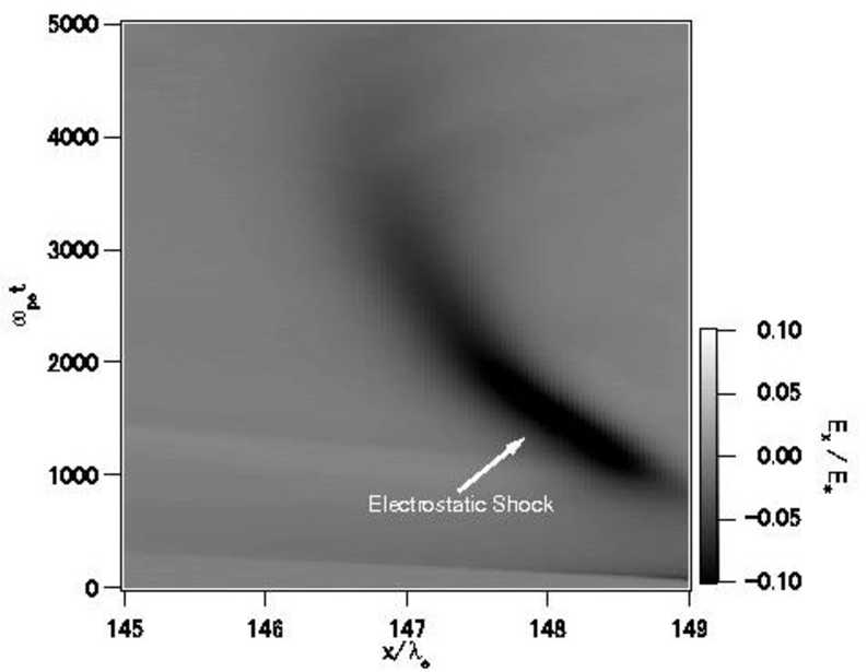
After $\omega_{\mathrm{pe}}t=2000$, however, the shock slows down and finally fades away. Figure 4 shows snapshots of the ion number density at $\omega_{\mathrm{pe}}t=1500$, $3000$, and $5000$. It is evident that oblique filamentary structures develop in front of the shock where the plasma is under the counter-streaming condition due to the existence of the reflected ions. We see that with the development of the filaments, the upstream plasma is strongly fluctuated and the shock structure is significantly modified. A similar structure was also observed in the simulation by Karimabadi, Omidi & Quest [22].

Figure 5 shows the charge density at $\omega_{\mathrm{pe}}t=3000$ and its power spectrum, which is directly related with the existence of the electrostatic modes. Comparing the region where the power is large in the power spectrum with that in the growth rate map obtained by the linear theory shown in Fig. 1, it is clear that these are generated by the electrostatic ion-ion instability. Note that, as is shown later, in fact the number density of the reflected ions is smaller than that of the incoming ions. The ratio is typically $0.6$ [see Fig. 8 (d)]. However, the growth rate as a function of $k_{x}$ and $k_{y}$ (not shown here) is not significantly different from that of the symmetric beam case shown in Fig. 1; the maximum growth rate is obtained as $\Gamma=2.4\times 10^{-3}\omega_{\mathrm{pe}}$ at $|k|=7.6\ \omega_{\mathrm{pe}}c^{-1}$ and $\theta=79^{\circ}$, which is only slightly smaller than the symmetric case.

Figure 6 shows the phase-space plots of the ions and electrons at $\omega_{\mathrm{pe}}t=1500$, $3000$, and $5000$. The thermal velocity of the ions in the upstream region increases with time in both $x$ and $y$ directions, while the increase in the velocity dispersion of the electrons is relatively small.

Figure 7 shows the time evolution of the velocity distributions of the ions within $143<x/\lambda_{\mathrm{e}}<145$, just in front of the shock front. The ions are heated especially in the $y$ direction because the electric field generated by the electrostatic ion-ion instability is almost directed in the $y$-direction. Thus, the anisotropy in the ion temperature increases with time.

There are two possible causes for the shock decay: one is the anisotropy in the ion temperature (or the decrease in the electron-to-ion temperature ratio), and the other is the fluctuation of the upstream plasma; both are caused by the electrostatic ion-ion instability. The time evolution of the temperatures immediately in front of the shock are shown in Fig. 8 together with that of the ratio of the reflected ion density to the incoming ion density. Here, the temperatures are calculated for the particles within the region in front of the shock given by

where we take $x_{\mathrm{sh}}(t)=-V_{\mathrm{sh,d}}(t-1000\omega_{\mathrm{pe}}^{-1})+148.5\lambda_{\mathrm{e}}$ and $V_{\mathrm{sh,d}}=1.2\times 10^{-3}c$ from Fig. 3. For the ions, we distinguish the “incoming ions” that have $v_{x}>0$ and the “reflected ions” that have $v_{x}<0$, while the electrons are regarded as a single population because the mean (bulk) velocity of the electrons are negligible compared to their thermal velocity. Since the electrostatic shock is formed at $\omega_{\mathrm{pe}}t\sim 1000$, the temperatures before that time are meaningless as those in front of the shock. We see that the electrons are heated in the $x$ and the $y$ directions in front of the shock immediately after the shock formation and then each component of the electron temperature keeps almost constant. On the other hand, the temperatures in the $y$-direction for both the incoming ions and the reflected ions rapidly increase with time within the period $1800<\omega_{\mathrm{pe}}t<2300$, which coincides with the period of the shock decay, while the other components do not change significantly. The ion heating in the $y$-direction would be caused by the electrostatic ion-ion instability and results in the anisotropic temperatures in the ions as well as the reduction of the electron-to-ion temperature ratio.

To clarify whether the anisotropic temperature in the ions is the cause of the shock decay, we carried out another (quasi) one-dimensional simulation with an anisotropic ion temperature. The simulation code used is the same two-dimensional code but we take only 8 grids in the $y$-direction so that the simulation is essentially one-dimensional; in such a simulation, since the electrostatic ion-ion instability does not develop, we can investigate the pure effect of the anisotropy in the ion temperature on the shock formation. For the shock formation, the condition of the incoming ions is more important than that of the reflected ions and Fig. 8 (b) shows the typical anisotropic temperature of the incoming ions is given by $T_{\mathrm{i},y}\sim 2T_{\mathrm{i},x}$ around the time of the shock decay. Here, as a more severe case, we take $T_{\mathrm{i},y}=4T_{\mathrm{i},x}$ keeping the other parameters unchanged as in the two-dimensional simulation, that is, $T_{\mathrm{e}}/T_{\mathrm{i},x}=9$. The time evolution of the electric field $E_{x}$ is shown in Fig. 9 (a). We found that the electrostatic shock forms under even this condition, where the shock speed measured in the upstream frame is $V_{\mathrm{sh}}\sim 1.2\times 10^{-2}c$ and the Mach number is given by $M_{\mathrm{s}}\sim 3.5$.

To confirm that the decrease in the electron-to-ion temperature ratio with isotropic ion temperature is also not the cause of the shock decay, we performed another quasi one-dimensional simulation with an isotropic ion temperature but the lower electron-to-ion temperature ratio of $T_{\mathrm{e}}/T_{\mathrm{i}}=4$. The result is shown in Fig. 9 (b) showing that the shock is also formed with even this temperature ratio at almost the same shock velocity and the Mach number as the anisotropic case. Thus, the anisotropic temperature in the ions nor the decrease in the temperature ratio are not the cause of the shock decay observed in the two-dimensional simulation.

For completeness, we also performed another quasi one-dimensional simulation with the same parameters as the two-dimensional one, that is, $T_{\mathrm{e}}/T_{\mathrm{i}}=9$, except the grid number in the $y$-direction. We found that the electrostatic shock forms and propagates without decaying in this case as well (not shown) confirming that the shock decay is a multi-dimensional effect.

Figure 10 shows the electrostatic potentials, the number density of the incoming ions, and that of the reflected ions at $\omega_{\mathrm{pe}}t=2000$ for the two-dimensional simulation. The potentials are normalized by the upstream ion kinetic energy ($m_{\mathrm{i}}V^{2}/2$). It is evident that the large potential fluctuation, which reaches even a half of the shock potential, exists in front of the shock due to the electrostatic ion-ion instability. Because of this electrostatic potential, the densities of both incoming and reflected ions are significantly disturbed where the fluctuation pattern almost traces the waves of the electrostatic ion-ion instability. In particular, it can be seen that the portions where the incoming ions enter the “shock front” are different from those where the ions are reflected toward upstream from the “front”.

Figure 11 shows the $y$-$v_{y}$ phase space distribution of the ions around $x\sim 145.5\lambda_{\mathrm{e}}$. The feature of the ion trapping [22, 31] is clear and therefore the fluctuation of the ion densities is a result of the nonlinear evolution of the electrostatic ion-ion instability. Thus, it can be concluded that the cause of the decay of the electrostatic shock is the large fluctuation in the ion density due to the electrostatic ion-ion instability.

In Fig. 10 (c), we can also find another interesting feature in the reflected ion density that is seen as a discontinuity around $x\sim 140\lambda_{\mathrm{e}}$, which could also be found in Fig. 4 (a). The $x$-$v_{x}$ phase space distribution of the ions is plotted in Fig. 12. As is shown in the panel (a), there is a structure in the phase space of the reflected ions around $x\sim 140\lambda_{\mathrm{e}}$. The panel (b) shows the close-up of this structure. We see that some of the reflected ions are reflected again there in the opposite direction. This structure would also be another electrostatic shock in which the upstream region is the larger $x$ side. This ‘secondary’ electrostatic shock would be formed as a result of that the faster reflected ions run into the slower ones from behind.

As was shown in Sec. II, the beam-Weibel instability can develop in counter-streaming plasmas with the wave vector in the $y$-direction as well as the electrostatic ion-ion instability. However, the large anisotropy in the ion temperature ($T_{\mathrm{i},y}/T_{\mathrm{i},x}\sim 2$ for the incoming ions and $T_{\mathrm{i},y}/T_{\mathrm{i},x}\sim 6$ for the reflected ions) caused by the electrostatic instability can affect the growth of the beam-Weibel instability. In addition, this temperature anisotropy itself may also cause the (ordinary) Weibel instability that has the wave vector in the $x$-direction. Here, let us consider the linear dispersion relation of these two Weibel-type instabilities in the anisotropic Maxwellian beam system given by the following zeroth-order distribution functions:

where $a_{\mathrm{s}x}$, $a_{\mathrm{s}y}$ and $a_{\mathrm{s}z}$ are the anisotropic thermal velocities for the respective directions of the species s. In the following, we consider the beams are symmetrical for simplicity, that is, $n_{e+}=n_{e-}=n_{i+}=n_{i-}=n_{\mathrm{e0}}$, $V_{\mathrm{e+}}=V_{\mathrm{i+}}=V$ and $V_{\mathrm{e-}}=V_{\mathrm{i-}}=-V$, as in Sec. II. Under this condition, the linear dispersion relation of the beam-Weibel instability with the wave vector in the $y$-direction is given by

where $\zeta_{\mathrm{s}}\equiv\omega/ka_{\mathrm{s}y}$. On the other hand, the linear dispersion relation of the (ordinary) Weibel instability with the wave vector in the $x$-direction is given by

where $\eta_{\mathrm{s}}\equiv(\omega/k-V_{\mathrm{s}})/a_{\mathrm{s}x}$. (Note that when $V=0$, this relation is reduced to that derived by Weibel [24] without the background magnetic field.) Figure 13 shows the growth rates of the two modes. We take here $T_{\mathrm{i},y}/T_{\mathrm{i},x}=4$, $T_{\mathrm{i},z}=T_{\mathrm{i},x}$ and $T_{\mathrm{e}}/T_{\mathrm{i},x}=9$ as typical values and the other parameters are the same as those of the initial condition of the two-dimensional simulation. As a reference, the growth rate for the isotropic beam case with $T_{\mathrm{e}}/T_{\mathrm{i}}=9$ discussed in Sec. II is also shown in the figure. We see that the growth rate of the beam-Weibel instability is reduced compared with that of the isotropic beam case due to the temperature anisotropy in the ions. Under this condition, the Weibel mode with the wave vector in the $x$-direction is stable and does not grow. (Of course, in the limit $V\to 0$, this mode should be unstable. We confirmed that it is unstable for $V<1.15\times 10^{-3}c$ for the same parameters.)

Figure 14 shows the $z$-component of the magnetic field, $B_{z}$, obtained from the two-dimensional simulation at $\omega_{\mathrm{pe}}t=1500,\ 3000,$ and $5000$. We see that the magnetic field grows with time with a wavelength comparable with that derived by the linear analysis ($\sim 40\lambda_{\mathrm{e}}$), although it may be affected by the periodic boundary condition because the wavelength is comparable with the system length in the $y$-direction. At this time ($\omega_{\mathrm{pe}}t\sim 5000$), the typical magnetic field strength is $|B|/B_{*}\sim 2\times 10^{-2}$ and the corresponding ion gyro-radius is given by $\sim 9\times 10^{2}\lambda_{\mathrm{e}}$; therefore, the ions are hardly deflected by this magnetic field. However, in the Weibel-type instability, the magnetic field is generated by the current filaments and the current filaments coalesce each other to grow larger filaments with stronger magnetic fields until saturation [32, see e.g.,]. Although, because of the limitation of the simulation box, we cannot study the further evolution of the filaments in this simulation, in the real world or in much larger simulations, the magnetic field would grow much stronger with the coalescence of the filaments and, long after the electrostatic shock vanished, it would become strong enough to form the “Weibel-mediated” shocks, a kind of collisionless shocks that dissipates the upstream particle kinetic energy via the magnetic field generated by the instability in the shock transition region.

As is reported in our previous paper of Ref. [29], we have performed a PIC simulation of the Weibel mediated shock with the larger flow velocity ($V=0.45c$) and the smaller mass ratio ($m_{\mathrm{i}}/m_{\mathrm{e}}=20$) with the equal temperatures for the electrons and the ions. (In that simulation, the electrostatic shock and the electrostatic ion-ion instability do not develop.) To illustrate the formation of the Weibel-mediated shock qualitatively, the time evolutions of the ion number density and the magnetic field ($z$-component) are shown in Fig. 15. The figures show the ion current filaments develop with time due to the beam-Weibel instability and finally the Weibel-mediated shock forms at $\omega_{\mathrm{pe}}t=2000$. Note that due to the mass ratio and the flow velocity, the temporal and spatial scales are different from those in the system with the real mass ratio of $m_{\mathrm{i}}/m_{\mathrm{e}}=1836$ and the slower flow speed $\sim 3000$ km s^-1. Returning to the situation of the present study, the ion current filaments developing around the electrostatic shock (Fig. 14) would also grow further and finally will evolve into the Weibel-mediated shock in the real world or in the simulations with much larger spatial and temporal scales.