From gene trees to species trees II:
Species tree inference in the deep coalescence model

Gene trees are fundamental to molecular systematics. Traditionally, a gene tree is reconstructed from DNA sequence variation at individual genetic loci in a group of species and is taken as the phylogenetic tree of the species due to sequencing technology limitations. However, when gene copies are sampled from various species, the resulting gene tree might disagree with the species tree. As such, the relationship between gene trees and species trees has been the focus of many studies (see for example [5, 12, 20, 25, 27, 31, 33]). It has long been recognized that gene trees can be used to estimate species divergence time, ancestral population sizes and even the containing species tree although they may not accurately reflect the species tree [7, 15, 21].

The discord of gene trees and the containing species tree can arise from horizontal gene transfer, lineage sorting, and gene duplication and loss. The importance of these causes depends on the considered genes and species. Hence, inferring the species tree from gene trees has been investigated under various parsimony criteria. With lineage sorting (also called deep coalescence), the problem is to find the tree minimizing extra gene lineages that had to coexist along species lineages [20]; with gene duplication, it becomes to find the tree minimizing gene duplications and/or losses [12, 25, 13, 28].

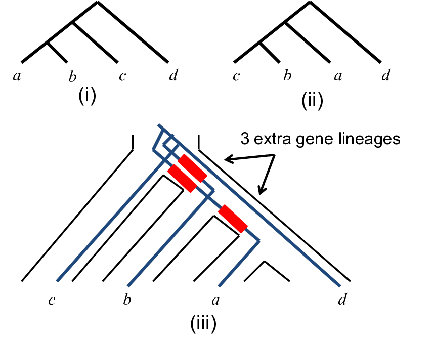
Inferring the species tree from a set of gene trees has often been studied under the gene duplication cost [1, 2, 3, 6, 8, 14, 16, 18, 30, 34] until very recently. In a seminal work [20], Maddison addressed lineage sorting in the framework of coalescence theory. Coalescence theory is an active branch of population genetics concerned with tracing the genealogical history of a present-day gene copy. For a gene sampled from two individuals, one may ask: How deep in time do these two lineages coalesce? Hence, the depth of this coalescence is a measure of the relationship between two sampled gene copies. The more deep in time coalescence occurs, the more distantly related they are. Maddison proposed to use the total number of “extra” gene lineages that fails to coalesce on a species tree to measure the inconsistence of a gene tree and species tree, called deep coalescence cost. For the gene tree and species tree shown in Figure 1, there are three gene lineages on a branch and two gene lineages on another branch that fail to coalesce, giving the deep coalescence cost of 3. Since coalescence theory provides the probability that a gene tree would exist in a species tree, it allows the inference problem to be studied in explicit statistical framework [4, 29]. This seems to give the deep coalescence model an advantage over the other models.

The paper is a sequel of [19], which studies the complexity and algorithmic issues of inferring the species tree from a set of gene trees with the gene duplication/loss cost. In this work, we present a relationship of the deep coalescence cost, the duplication cost, and the number of gene losses. Although deep coalescence and gene duplication are two different mechanisms responsible for the discord of gene trees and species trees, this relationship suggests that the deep coalescence cost and the duplication cost are closely related to each other as a similarity measure of trees. We further show that inferring species tree from gene trees is also NP-hard by minimizing the deep coalescence cost.

In this section, we shall introduce basic definitions and notations on gene duplication, gene loss and deep coalescence that are used in the following sections.

We have seen that deep coalescences, gene losses and duplications are inferred through the gene tree/speceis tree reconciliation. Actually, they are indeed closely related through a simple equation.

Note that type-2 or type-3 internal nodes correspond one-to-one with duplication events.

Proof. Let $G$ and $S$ have $n$ leaves. Assume that there are $k_{1}$ type-1 internal nodes

$k_{2}$ type-2 internal nodes

and $k_{3}$ type-3 internal nodes

in $G$ under the lca mapping $M:G\rightarrow S$, respectively. Since $G$ is a full binary tree with $n$ leaves, $G$ has $n-1$ internal nodes and hence

Additionally, type-2 and type-3 nodes correspond one-to-one with duplication events,

For simplicity, we assume that $g^{\prime}$ and $g^{\prime\prime}$ are the children of $g$ for each type-1 internal node $g$; we also assume that $a(g)$ is the unique child such that $M\left(a(g)\right)\subset M(g)$ for each type-2 node $g$. Since we use $d\left(M(h),M(g)\right)$ to denote the number of nodes on the path from $M(g)$ to $M(h)$ for a node $g$ and its child $h$, the number of lineages contained in the path is $d\left(M(h),M(g)\right)+1$. Therefore, by Eqn. (3) and (4) and the fact that $|E(S)|=2n-2$,

This concludes the proof. $\Box$

(2) Since the number of gene duplications and lossed can be calculated in linear time [34, 19], the first remark implies that the deep coalescence cost can also be computed in linear time.

By Thm 3.1, $c_{dc}(G,S)\leq c_{loss}(G,S)$ for a species tree $S$ and a uniquely leaf labeled gene tree $G$. Now we show that it is bounded below by the duplication cost for any arbitrary gene tree.

Proof. Denote the image node set of the lca mapping $M$ by $M(G)$, which is a subset of nodes in the species tree $S$. For any internal node $s\in M(G)$, we use $M^{-1}(s)$ to denote all internal nodes $g$ of the gene tree that are mapped to $s$ under $M$. For any nodes $x$ and a descendant $y$ of $x$ in the gene tree $G$, if $M(x)=M(y)=s$, then $M(g)=s$ for each node in the path from $x$ to $y$. Since $G$ is uniquely leaf labeled, all internal nodes in $M^{-1}(s)$ form a rooted subtree of $G$, denoted by $T^{-1}(s)$, as illustrated in Figure 2.

$T^{-1}(s)$ is not a full binary tree in general. In particular, its root might has degree 1. Let $n^{\prime}_{s},n^{\prime\prime}_{s},n^{\prime\prime\prime}_{s}$ denote the number of non-root degree-1, degree-2 and degree-3 nodes in the subtree $T^{-1}(s)$, respectively. Assume that $T^{-1}(s)$ has two or more nodes. Then, by definition, the root of $T^{-1}(s)$ corresponds with a gene duplication in the reconciliation of $G$ and $S$; each degree-2 or degree-3 node of $T^{-1}(s)$ also corresponds with a gene duplication. Therefore, there are $n^{\prime\prime}_{s}+n^{\prime\prime\prime}_{s}+1$ duplication events at $s$. We now consider two cases.

Case 1. The root of $T^{-1}(s)$ has degree 1. Then $T^{-1}(s)$ has $n^{\prime\prime\prime}_{s}+1$ leaves, that is $n^{\prime}_{s}=n^{\prime\prime\prime}_{s}+1$. For each leaf of $T^{-1}(s)$, it has two children that are mapped to a node below $s$ in the species tree $S$; each non-root degree-2 node has exactly one child that is mapped to a node below $s$ and so is the root since it has degree 1. Thus, there are $2\left(n^{\prime\prime\prime}_{s}+1\right)+n^{\prime\prime}_{s}+1$ image paths that contain one of the two lineages from $s$ to one of its children.

Case 2. The root has degree 2. In this case, $T^{-1}(s)$ has $n^{\prime\prime\prime}_{s}+2$ leaves and there are $2\left(n^{\prime\prime\prime}_{s}+2\right)+n^{\prime\prime}_{s}$ image paths that contain one of the two lineages from $s$ to one of its children.

By distributing the DC and duplication costs to each image node $s$ in $M(G)$, we obtain that

This finishes the proof. $\Box$

Parsimony criterion is often used for inference in biology. Hence, inferring species tree from a set of gene trees is formulated as the following algorithmic problem

It is proved that the species tree problem is NP-hard for the duplication and/or loss cost in [19]. In this section, we prove the following theorem.

Proof. Given a gene tree $G$ and a species tree $S$, the DC cost $c_{dc}(G,S)$ can be computed in polynomial time since gene duplications and losses can be counted in linear time [34]. Therefore, the species tree problem is in NP.

To prove its NP-hardness, we reduce the Maximum Cut problem to the decision version of the species tree problem. Given an instance graph ${\cal G}=(V,E)$ and a positive integer $I$, the Maximum Cut problem is to partition the node set $V$ into two disjoint subsets $V_{1}$ and $V_{2}$ such that there are at least $I$ edges from $E$ that have one endpoint in $V_{1}$ and one endpoint in $V_{2}$. Assume that $V=\{v_{1},v_{2},\cdots,v_{n}\}$ and $|E|$ denotes the number of edges from $E$, where $n>3$. We construct a corresponding instance of the species tree problem as follows.

Choose $N>n^{2}$ and $M\geq n^{2}N(N+1)+|E|$. For each node $v_{i}$ ($1\leq i\leq n$), we introduce a label with the same name $v_{i}$. We also introduce $2N+M$ extra labels $x_{i},y_{i}$, $1\leq i\leq N$ and $z_{j}$, $1\leq j\leq M$. For each edge $e=(v_{i},v_{j})\in E$, we define two gene trees $T_{e1}$ and $T_{e2}$ as shown in Figure 3. These two trees are same except that the leaf labels $v_{i}$ and $v_{j}$ are swapped.

Let the trees shown in Figure 4 (i)-(iii) be written as $L[x_{i},x_{j},y_{k},z_{l}]$, $L[y_{i},y_{j},x_{k},z_{l}]$ and $F[\{x_{i}\},\{y_{i}\},z_{l}]$, respectively. Besides the ‘edge’ gene trees $T_{e1}$ and $T_{e2}$ ($e\in E)$, the set $\cal A$ of gene trees in the instance of the problem to be defined also contains

These three classes of gene trees are introduced to restrict the topology of the optimal species tree for the defined instance of the problem. Hence, we call them ‘structural’ gene trees. The NP-completeness of the decision version of the species tree problem follows from the following two lemmas.

Proof. Assume that the node set $V$ of the graph $\cal G$ divides into $V_{1}=\{v_{1},v_{2},\cdots,v_{p}\}$ and $V_{2}=\{v_{p+1},v_{p+2},\cdots,v_{n}\}$ such that there are exactly $d$ edges having one endpoint in $V_{1}$ and one endpoint in $V_{2}$. We define a species tree $S_{\cal G}$ as shown in Figure 5.

First, we observe that

for each possible $i,j,k,m$.

Consider a non-cut edge $e=(v_{i},v_{j})$ ($i<j$). Since $L(T_{e1})=L(T_{e2})\subset L(S_{\cal G})$, $c_{dc}(T_{e1},S_{\cal G})=c_{dc}(T_{e1},S_{\cal G}|_{L(T_{e1})})$ and $c_{dc}(T_{e2},S_{\cal G})=c_{dc}(T_{e2},S_{\cal G}|_{L(T_{e2})})$. If $v_{i},v_{j}\in V_{1}$, we have that

Symmetrically, if $v_{i},v_{j}\in V_{2}$, we have that

For each cut edge $e=(v_{i},v_{j})$ ($i<j$) with one endpoint in $V_{1}$, say $v_{i}\in V_{1}$, and another in $V_{2}$, we have that

Therefore, we have

This finishes the proof of the lemma. $\Box$

Proof. If $t>|E|$, the fact is trivial. Hence, without loss of generality, we may assume that $t\leq|E|$. Here, we use $\mbox{LTree}[a,\ldots,b,c]$ to denote the line tree with leaves labeled by $a$, $b$, $\ldots$, $c$, respectively, as shown in Figure 6 (i). Note that the leaf $a$ is a child of the root in $\mbox{LTree}[a,\ldots,b,c]$. For a set of trees $T^{\prime}$, $T^{\prime\prime}$, $\ldots$, $T^{\prime\prime\prime}$, we use

to denote the tree obtained by replacing each leaf by a corresponding subtree in $\mbox{LTree}[a,\ldots,b,c]$ as shown in Figure 6 (ii).

Let $B$ be a subset of leaves in the species tree $S$ and the least common ancestor of the leaves from $B$ be $r_{B}$ in $S$. Recall that the homomorphic subtree $S|_{B}$ of $S$ induced by $B$ is the tree obtained from $S$ by removing all the nodes and edges that are not on a path from $r_{B}$ to a leaf from $B$ and then contracting all the degree-2 node except for the root $r_{B}$. For example, for $S_{\cal G}$ defined in Lemma4.1, $S_{\cal G}|_{\{x_{1},x_{2},y_{1}\}}=\mbox{LTree}[y_{1},x_{1},x_{2}]$.

Set

By replacing the children of a two-leaf root tree with $S|_{U}$ and $S|_{Z}$, we obtain a species tree $S^{\prime}=\mbox{LTree}[S|_{U},S|_{Z}]$ from S. First, $S^{\prime}$ has the following property.

Similarly, we also have the following three inequalities

for any $i,j,k,m$. Thus, the fact holds. $\Box$

Let $X=\{x_{1},x_{2},\ldots,x_{N}\}$ and $Y=\{y_{1},y_{2},\ldots,y_{N}\}$. Then $S^{\prime}|_{X}=(S|_{U})|_{X}$ and $S^{\prime}|_{Y}=(S|_{U})|_{Y}$.

Let the least common ancestor of $x_{i}$s and $y_{i}$s be $r$ in $S^{\prime}$. We have shown that $x_{i}$s are below one child of $r$, say $r_{1}$, and $y_{i}$’s are below the other child of $r$, say $r_{2}$. In addition, $S^{\prime}|_{X}$ and $S^{\prime}_{Y}$ are two line trees.

Case 1. $S|_{X\cup\{v_{i},v_{j}\}}=\mbox{LTree}[x_{1},x_{2},\cdots,x_{k},v_{i},x_{k+1},\cdots,x_{m},v_{j},v_{m+1},\cdots,x_{N}]$ for some $0\leq k\leq m\leq N$. In this case, we have that

and

Hence,

as the minimum value of $(N-k)(N-k-1)+2k+2$ is $N$ (reaching at $k=N-2,N-1$).

Case 2. $S|_{X\cup\{v_{i},v_{j}\}}=\mbox{LTree}[x_{1},x_{2},\cdots,x_{k},\mbox{LTree}[v_{i},v_{j}],x_{k+1},\cdots,x_{N-1},x_{N}]$ for some $0\leq k\leq N$. We have that

and so

References

- [1] Bansal MS and Eulenstein O (2008) The multiple gene duplication problem revisited. Bioinformatics 24:132-138.
- [2] Chauve C, Doyon JP, El-Mabrouk N (2008) Gene family evolution by duplication, speciation, and loss. J. Comput. Biol. 15:1043-1062.
- [3] Chen K, Durand D, Farach-Colton M (2000) Notung: A program for dating gene duplications and optimizing gene family trees. J Comput. Biol. 7:429-447.
- [4] Degnan JH, Salter LA (2005) Gene tree distribution under the coalescence process. Evolution 59:24-37.
- [5] Doyle JJ (1992) Gene trees and species trees: molecular systematics as one-character taxonomy. Syst. Bot. 17: 144-163.
- [6] Durand D, Halldorsson BV, Vernot B (2006) A hybrid micro-macroevolutionary approach to gene tree reconstruction. J. Comput. Biology 13:320-335.
- [7] Edwards SV, Beerli P (2000) Perspective: gene divergence, population divergence, and the variance in coalescence time in phylogeography studies. Evolution 54: 1839–1854.
- [8] Eulenstein O, Mirkin B, Vingron M (1998) Duplication-based measures of difference between gene and species trees. J. Comput. Biol. 5:135-148.
- [9] Stege U (1999) Gene Trees and Species Trees: The Gene-Duplication Problem in Fixed-Parameter Tractable. In Proceedings of WADS, pp. 288-293
- [10] Fitch W (1970) Distinguishing homologous from analogous proteins. Syst. Zool. 19:99-113.
- [11] Garey M, Johnson D (1979) Computers and Intractability: A Guide to the Theory of NP-completeness, W. H. Freeman, New York.
- [12] Goodman M, Czelusniak J, Moore GW, Romero-Herrera AE, Matsuda G (1979) Fitting the gene lineage into its species lineage, a parsimony strategy illustrated by cladograms constructed from globin sequences, Syst. Zool. 28:132-163.
- [13] Guigó R, Muchnik I, Smith T (1996) Reconstruction of ancient molecular phylogeny, Mol. Phy. and Evol. 6:189-213.
- [14] Hallett MT, Lagergren J (2000) New algorithms for the duplication-loss model. In Proceedings of RECOMB’2000, pp. 138-146.
- [15] Hey J, Nielsen R (2004) Multilocus methods for estimating population sizes, migration rates and divergence time, with applications to the divergence of Drosophila pseudoobscura and D. persimilis. Genetics 167:747-760.
- [16] Libeskind-Hadas R and Charleston MA (2009) On the computational complexity of the reticulate cophylogeny reconstruction problem, J. Comput. Biol. 16:105-117.
- [17] Liu L, Yu LL, Kubatko L, Pearl DK, Edwards SV (2009) Coalescent methods for estimating phylogenetic trees. Mol. Phylogenet. Evol. 53:320-328.
- [18] Luo CW, Chen MC, Chen YC, Yang WL, Liu HF, Chao KM, Linear-time algorithms for the multiple gene duplication problems. IEEE Trans. Comput Biol. and Bioinform. (in press).
- [19] Ma B, Li M, Zhang LX (2001) From gene trees to species trees. SIAM J. Comput. 30:729-752
- [20] Maddison WP (1997) Gene trees in species trees, Syst. Biol. 46:523-536.
- [21] Maddison WP, Knowles L (2006) Inferring phylogeny despite incomplete lineage sorting. Syst. Biol. 55: 21-30.
- [22] Mirkin B, Muchnik I, Smith T (1995) A biologically meaningful model for comparing molecular phylogenies, J. Comput. Bio. 2:493-507.
- [23] Miyamoto MM, Fitch WM (1995) Testing species phylogenies and phylogenetic methods with congruence. Syst. Biol. 44:64-76.
- [24] Nei M (1987) Molecular Evolutionary Genetics, Columbia University Press, New York.
- [25] Page R (1994) Maps between trees and cladistic analysis of historical associations among genes, organisms, and areas. Syst. Bio. 43:58-77.
- [26] Page R, M. Charleston MA (1997) From gene to organismal phylogeny: reconciled trees and the gene tree/species tree problem. Mol. Phy. and Evol. 7:231-240.
- [27] Pamilo P, Nei M (1988) Relationship between gene trees and species trees, Mol. Biol. Evol. 5:568-583.
- [28] Ronquist F (1997) Phylogenetic approaches in coevolution and biogeography Zool. Scripta 26: 313-322
- [29] Rosenberg NA (2002) The probability of topological concordance of gene trees and species trees. Theor. Pop. Biol. 61:225-247.
- [30] Roth C, Rastogi A, Arvestad L, Dittmar K, Light S, Ekman D, David A. Liberles DA (2007) Evolution after gene duplication: models, mechanisms, sequences, systems, and organisms J Exp. Zool. Part B 308B: 58-73.
- [31] Takahata N (1989) Gene genealogy in three related population: Consistency probability between gene and population trees. Genetics 122:957-966.
- [32] Than C, Nakhlen L (2009) Species tree inference by minimizing deep coalescences. PLoS Comput. Biol. 5:e1000501.doi:10.1371/journal.pcbi.1000501.
- [33] Wu C-I (1991) Inference of species phylogeny in relation to segregation of ancient polymorphisms. Genetics 127:429-435.
- [34] Zhang LX (1997) On a Mirkin-Muchnik-Smith conjecture for comparing molecular phylogenies. J. Comput. Biol. 4:177-188.