跳到论文正文
W Papers独立论文阅读器 arXiv:1003.1192 论文正文 计算阅读时间 · 0%
引用这篇论文根据当前论文元数据生成,正式投稿前建议核对。


License: arXiv.org perpetual non-exclusive license
arXiv:1003.1192v2 [hep-th] 18 Aug 2010

IPhT-t10/026

{centering}The classical RR-matrix of AdS/CFT

and its Lie dialgebra structure

Benoît Vicedo

Laboratoire de Physique Théorique, École Normale Supérieure
24 rue Lhomond, 75231 Paris CEDEX-5, France

and

Institut de Physique Théorique, C.E.A. - Saclay,
F-91191 Gif-sur-Yvette, France

benoit.vicedo@cea.fr

{centering}

The classical integrable structure of ℤ4\mathbb{Z}_{4}-graded supercoset σ\sigma-models, arising in the AdS/CFT correspondence, is formulated within the RR-matrix approach. The central object in this construction is the standard RR-matrix of the ℤ4\mathbb{Z}_{4}-twisted loop algebra. However, in order to correctly describe the Lax matrix within this formalism, the standard inner product on this twisted loop algebra requires a further twist induced by the Zhukovsky map, which also plays a key role in the AdS/CFT correspondence. The non-ultralocality of the σ\sigma-model can be understood as stemming from this latter twist since it leads to a non skew-symmetric RR-matrix.

1 Introduction and summary

Since the early days of the ongoing study of the AdS5/CFT4 conjecture [1] in the planar sector, footprints of integrability were discovered both in gauge theory [2, 3, 4] where the ’t Hooft coupling λ≪1\lambda\ll 1 is very small as well as in string theory [5] where λ≫1\lambda\gg 1, hinting at the existence of a deep underlying integrable structure at all intermediate values λ∼1\lambda\sim 1. In light of these encouraging discoveries, the generally favoured approach thus far has been a top-down one, whereby quantum integrability was assumed and its implications could be subsequently tested against perturbative data from both sides of the correspondence.

Indeed, in the infinite volume limit L≫1L\gg 1 where scattering makes sense, the notion of quantum integrability in (1+1)(1+1)-dimensions essentially reduces to the factorisability of the 𝒮\mathcal{S}-matrix. Thus regardless of the details of the hypothetical integrable structure at λ∼1\lambda\sim 1, in the limit L→∞L\rightarrow\infty the central object becomes the 2→22\to 2 𝒮\mathcal{S}-matrix. In the fundamental representation, the latter could be determined from its invariance under the maximal central extension 𝔥≔𝔭​𝔰​𝔲​(2|2)⋉ℝ3\mathfrak{h}\coloneqq\mathfrak{psu}(2|2)\ltimes\mathbb{R}^{3} of the residual symmetry algebra [6] and such that it satisfies the requirements of unitarity, crossing symmetry and the quantum Yang-Baxter equation [7]. When expressed in terms of ℛ=P​𝒮\mathcal{R}=P\mathcal{S}, where PP is a permutation, these properties suggest the existence of a subjacent Yangian based on 𝔥\mathfrak{h} [8]. Yet no universal ℛ\mathcal{R}-matrix for the non-semisimple algebra 𝔥\mathfrak{h} has yet been identified. However, the classical limit λ≫1\lambda\gg 1 of this hypothetical universal ℛ\mathcal{R}-matrix, namely a universal classical rr-matrix with its associated Lie bialgebra structure, was conjectured in [9].

On the CFT side of the story, the 1-loop dilatation operator of planar 𝒩=4\mathcal{N}=4 SYM theory was identified with the Hamiltonian of an integrable spin-chain [2], a property which seems to persist also at higher loops [3]. Subsequent investigations of the integrable structure of planar 𝒩=4\mathcal{N}=4 SYM theory revealed that the dilatation operator admits, at the first few orders of perturbation theory, a Yangian symmetry based on the full 𝔭​𝔰​𝔲​(2,2|4)\mathfrak{psu}(2,2|4) algebra [4]. This symmetry, however, is exact only in the infinite spin-chain limit L≫1L\gg 1 due to usual violation of boundary conditions by the Yangian. It is natural to expect that this Yangian structure contains the Yangian of 𝔥\mathfrak{h} arising from the 𝒮\mathcal{S}-matrix as a subalgebra, at least when acting on physical asymptotic states.

At the AdS end of the spectrum, which we shall focus on, the first signs of integrability in classical superstring theory on A​d​S5×S5AdS_{5}\times S^{5} came with the discovery of the Bena-Polchinski-Roiban (BPR) Lax connection [5]. The classical Yangian generated by the corresponding first non-local charges was identified in [10]. Later on, the Poisson bracket of this Lax connection could be brought into a form exhibiting integrability [11], although only in various bosonic subsectors admitting a principal chiral model representation [12]. Earlier attempts at bringing the Poisson structure of the full superstring on A​d​S5×S5AdS_{5}\times S^{5} into the desired form had been either inconclusive [13] or only partially satisfactory [14]. It was only much later, after adding to the BPR Lax connection extra terms proportional to various Hamiltonian constraints (see [15] for a justification of this extension), that this program was finally brought to completion [16].

The resulting classical integrable structure, valid at finite-volume, is characterised by a pair of r/sr/s-matrices [11] which generalise the standard notion of classical rr-matrix for so called ‘ultralocal’ systems to the ‘non-ultralocal’ case at hand. A remarkable, and yet quite surprising, fact is that one obtains the same kind of r/sr/s-algebra with the exact same rr- and ss-matrices whether one works within the Green-Schwarz or the pure spinor formalism of the superstring on A​d​S5×S5AdS_{5}\times S^{5} [15, 16]. This suggests a unified approach for quantising the superstring starting from this r/sr/s-algebra.

The purpose of this paper is to reformulate the classical integrable structure of the superstring σ\sigma-model within the RR-matrix approach [17], in which the pair of r/sr/s-matrices admit a very natural and simple algebraic interpretation. In fact, it is by now well understood that the special property of superstrings on A​d​S5×S5AdS_{5}\times S^{5} guaranteeing its classical integrability is the ℤ4\mathbb{Z}_{4}-grading of its supercoset target space [18]. We shall therefore work within the more general setting of ℤ4\mathbb{Z}_{4}-graded supercoset σ\sigma-models and exhibit their classical integrable structure and corresponding RR-matrix.

For conciseness we summarise the main result here. Let 𝔤\mathfrak{g} be the Grassmann envelope of a ℤ4\mathbb{Z}_{4}-graded Lie superalgebra 𝔤̊\mathring{\mathfrak{g}}, with ℤ4\mathbb{Z}_{4}-automorphism Ω\Omega, and consider its twisted loop algebra ℒ​𝔤Ω\mathcal{L}\mathfrak{g}^{\mbox{\scriptsize$\Omega$}} in the loop variable zz. This admits a natural vector space decomposition ℒ​𝔤Ω=ℒ​𝔤+Ω∔ℒ​𝔤−Ω\mathcal{L}\mathfrak{g}^{\mbox{\scriptsize$\Omega$}}=\mathcal{L}\mathfrak{g}^{\mbox{\scriptsize$\Omega$}}_{+}\dotplus\mathcal{L}\mathfrak{g}^{\mbox{\scriptsize$\Omega$}}_{-} into positive and negative powers of zz. Introduce the standard classical RR-matrix as the difference of projections onto these respective subspaces,

R=π+−π−∈End ​ℒ​𝔤Ω.R=\pi_{+}-\pi_{-}\in\text{End }\mathcal{L}\mathfrak{g}^{\mbox{\scriptsize$\Omega$}}. (ii)

The rr- and ss-matrices are then given by the skew-symmetric and symmetric parts of RR with respect to the standard inner product on ℒ​𝔤Ω\mathcal{L}\mathfrak{g}^{\mbox{\scriptsize$\Omega$}} ‘twisted’ by the Zhukovsky map z↦uz\mapsto u, namely

(X,Y)ϕ=resz⁡⟨X⁡(z),Y⁡(z)⟩​d​u,∀X,Y∈ℒ​𝔤Ω.(X,Y)_{\phi}=\res_{z}\langle X(z),Y(z)\rangle du,\qquad\forall X,Y\in\mathcal{L}\mathfrak{g}^{\mbox{\scriptsize$\Omega$}}. (i​iii)

Besides reproducing the correct r/sr/s-matrices, the need for twisting by the Zhukovsky map can also be seen from the very special form of the Lax matrix of the supercoset σ\sigma-model,

𝔏=4​ϕ​(z)−1​∑k=1∞zk​(k​A1(k)+2​(∇1Π1)(k)),\mathfrak{L}=4\,\phi(z)^{-1}\sum_{k=1}^{\infty}z^{k}\left(kA_{1}^{(k)}+2(\nabla_{1}\Pi_{1})^{(k)}\right), (i​i​iiii)

where {A1(i),∇1Π1(i)}i=03\{A_{1}^{(i)},\nabla_{1}\Pi_{1}^{(i)}\}_{i=0}^{3} are the fields of the σ\sigma-model and ϕ⁡(z)=z​∂zu\phi(z)=z\partial_{z}u. Indeed, after twisting the standard inner product by ϕ⁡(z)\phi(z), which results in ( ⁢ i i ), the Lax matrix ( ⁢ i i i ) admits a very natural description, namely it can be shown to take values in the smooth dual (ℒ​𝔤−Ω)∗(\mathcal{L}\mathfrak{g}^{\mbox{\scriptsize$\Omega$}}_{-})^{\ast}.

As we shall show in the core of the paper, all the necessary information about the classical integrable structure of the supercoset σ\sigma-model is contained in the RR-matrix ( i ), the inner product ( ⁢ i i ) and the Lax matrix ( ⁢ i i i ). Indeed, the RR-matrix ( i ) on ℒ​𝔤Ω\mathcal{L}\mathfrak{g}^{\mbox{\scriptsize$\Omega$}} lifts to the central extension 𝔊^\hat{\mathfrak{G}} of the current algebra C∞​(S1,ℒ​𝔤Ω)C^{\infty}(S^{1},\mathcal{L}\mathfrak{g}^{\mbox{\scriptsize$\Omega$}}) and the associated Poisson structure on its smooth dual 𝔊^∗\hat{\mathfrak{G}}^{\ast} then corresponds exactly to the r/sr/s-algebra of [16]. Moreover, the Lax matrix ( ⁢ i i i ) belongs to a certain coadjoint orbit in 𝔊^∗\hat{\mathfrak{G}}^{\ast} parameterised by finitely many functions on the circle S1S^{1}.

Remarks.

  • •

    We consider the Grassmann envelope 𝔤\mathfrak{g} of the Lie superalgebra 𝔤̊\mathring{\mathfrak{g}} for two reasons: firstly it is a Lie algebra and so the RR-matrix approach directly applies to it, and secondly it naturally exponentiates to the Lie group with Grassmann structure G≔exp⁡𝔤G\coloneqq\exp\mathfrak{g} which is the starting point for the construction of the supercoset σ\sigma-model action.

  • •

    The RR-matrix ( i ) satisfies the so-called modified classical Yang-Baxter equation, as a result of which [X,Y]R=12​([R​X,Y]+[X,R​Y]),∀X,Y∈ℒ​𝔤Ω[X,Y]_{R}=\mbox{\small$\frac{1}{2}$}([RX,Y]+[X,RY]),\forall X,Y\in\mathcal{L}\mathfrak{g}^{\mbox{\scriptsize$\Omega$}} defines a second Lie bracket on ℒ​𝔤Ω\mathcal{L}\mathfrak{g}^{\mbox{\scriptsize$\Omega$}}. We say that ℒ​𝔤Ω\mathcal{L}\mathfrak{g}^{\mbox{\scriptsize$\Omega$}} is a Lie dialgebra, to be distinguished from a Lie bialgebra which admits a second Lie bracket on its dual. When R∗=−RR^{\ast}=-R the two structures can be identified, however due to the twist in the inner product ( ⁢ i i ) this is not possible here.

  • •

    The r/sr/s-matrices of Schäfer-Nameki and Mikhailov [14] also admit an interpretation in the RR-matrix approach, albeit a more complicated one. Specifically it should be given by a sum of RR in ( i ) and a matrix R0R_{0} obtained from its projection onto the grade zero part of 𝔤\mathfrak{g}, much like the RR-matrix for a bosonic σ\sigma-model on a symmetric space found in [19].

  • •

    Let us also point out a possible connection with the classical rr-matrix of Beisert-Spill [9]. It too presents a form of twisiting similar to ( ⁢ i i ), but is based on the symmetry algebra 𝔤​𝔩​(2|2)\mathfrak{gl}(2|2) and generates a Lie bialgebra structure. Although the underlying algebras are different, it ought to be possible to relate the RR-matrix ( i ) for 𝔤̊=𝔭​𝔰​𝔲​(2,2|4)\mathring{\mathfrak{g}}=\mathfrak{psu}(2,2|4) in the large volume limit L≫1L\gg 1 to this classical skew-symmetric rr-matrix which describes asymptotic scattering.

  • •

    The construction presented here is entirely standard [17] apart from the twist in the inner product ( ⁢ i i ), which however was also used in [19]. The difference here is that the twist will appear naturally as a factor in the Lax matrix ( ⁢ i i i ), expressing the need for a corresponding twist in the inner product ( ⁢ i i ). A similar factor in the Lax matrix can also be found in [20], where it was explicitly applied to the case of the principal chiral model.

  • •

    Since the inner product enters in the definition of the Poisson structure, the latter therefore has a natural dependence on the Zhukovsky variable uu. This is in agreement with the earlier observation that the symplectic structure induced on the space of finite-gap solutions is canonical when expressed in the Zhukovsky variable [21].

  • •

    The integrable structure based on ( i ), ( ⁢ i i ) and ( ⁢ i i i ) does not rely on any specific properties of the Lie superalgebra 𝔤\mathfrak{g} other than that it should admit a ℤ4\mathbb{Z}_{4}-automorphism. The construction should therefore equally apply to all other AdS/CFT-type dualities based on ℤ4\mathbb{Z}_{4}-graded Lie superalgebras [22], as recently classified in [23].

  • •

    There is nothing special about ℤ4\mathbb{Z}_{4}-gradings since it is known that Lie (super)algebras with ℤm\mathbb{Z}_{m}-gradings also give rise to actions admitting a Lax connection [24]. It would be interesting to generalise the construction of the Hamiltonian Lax connection to this setting, compute the corresponding r/sr/s-matrices and interpret them in the RR-matrix approach.

The paper is organised as follows: In section 2 we introduce supercoset σ\sigma-models for a generic ℤ4\mathbb{Z}_{4}-graded Lie superalgebra 𝔤̊\mathring{\mathfrak{g}} and review the derivation of the Lax connection in the Hamiltonian setting. In section 3 we define the twisted loop algebra ℒ​𝔤Ω\mathcal{L}\mathfrak{g}^{\mbox{\scriptsize$\Omega$}} with its twisted inner product ( ⁢ i i ). In section 4 we equip ℒ​𝔤Ω\mathcal{L}\mathfrak{g}^{\mbox{\scriptsize$\Omega$}} with a Lie dialgebra structure by means of the standard RR-matrix ( i ). We construct the current algebra 𝔊\mathfrak{G} of ℒ​𝔤Ω\mathcal{L}\mathfrak{g}^{\mbox{\scriptsize$\Omega$}} in section 5, and show that its central extension 𝔊^\hat{\mathfrak{G}} gives rise to zero curvature type equations. In section 6 we show that 𝔊^\hat{\mathfrak{G}} inherits a Lie dialgebra structure from ℒ​𝔤Ω\mathcal{L}\mathfrak{g}^{\mbox{\scriptsize$\Omega$}} and that the corresponding Kostant-Kirillov Poisson structure on the dual 𝔊^∗\hat{\mathfrak{G}}^{\ast} is of the desired r/sr/s-type with the r/sr/s-matrices of [16]. Section 7 serves to reinterpret the results of [15] and [16] in the present formalism. We occasionally refer to appendix A for notations.

2 ℤ4\mathbb{Z}_{4}-graded supercoset σ\sigma-models

Lie superalgebra.

Let 𝔤̊\mathring{\mathfrak{g}} be a Lie superalgebra admitting a ℤ4\mathbb{Z}_{4}-automorphism Ω:𝔤̊→𝔤̊\Omega:\mathring{\mathfrak{g}}\rightarrow\mathring{\mathfrak{g}}, namely such that Ω4=1\Omega^{4}=1. As a vector space, 𝔤̊\mathring{\mathfrak{g}} then decomposes into a direct sum ⊕n=03𝔤̊n\oplus_{n=0}^{3}\mathring{\mathfrak{g}}_{n} of eigenspaces of Ω\Omega defined by Ω⁡(𝔤̊n)=in​𝔤̊n\Omega(\mathring{\mathfrak{g}}_{n})=i^{n}\mathring{\mathfrak{g}}_{n}. We shall also assume that 𝔤̊\mathring{\mathfrak{g}} admits a non-degenerate, invariant, graded-symmetric, bilinear form ⟨⋅,⋅⟩:𝔤̊×𝔤̊→ℂ\langle\cdot,\cdot\rangle:\mathring{\mathfrak{g}}\times\mathring{\mathfrak{g}}\rightarrow\mathbb{C} which moreover respects the grading in the sense that whenever x∈𝔤̊nx\in\mathring{\mathfrak{g}}_{n}, y∈𝔤̊my\in\mathring{\mathfrak{g}}_{m} we have ⟨x,y⟩=0\langle x,y\rangle=0 unless (n+m)=0(n+m)=0, where (n)≔n⁡(mod ​4)(n)\coloneqq n(\text{mod }4).

The Grassmann envelope 𝔤≔(Γ⊗𝔤̊)0¯\mathfrak{g}\coloneqq(\Gamma\otimes\mathring{\mathfrak{g}})_{\bar{0}} of 𝔤̊\mathring{\mathfrak{g}} is defined as the grade zero part of its tensor product with a Grassmann algebra Γ\Gamma. All the properties of 𝔤̊\mathring{\mathfrak{g}} extend naturally to 𝔤\mathfrak{g}, with the only difference being that ⟨⋅,⋅⟩:𝔤×𝔤→Γ0\langle\cdot,\cdot\rangle:\mathfrak{g}\times\mathfrak{g}\rightarrow\Gamma_{0} is now symmetric. Since 𝔤\mathfrak{g} is a Lie algebra, one can define its corresponding Lie group (with Grassmann structure) via the exponential map G≔exp⁡𝔤G\coloneqq\exp\mathfrak{g}.

Supercoset σ\sigma-model.

Let H≔exp⁡𝔤0H\coloneqq\exp\mathfrak{g}_{0} denote the Lie subgroup of GG corresponding to the Lie subalgebra 𝔤0\mathfrak{g}_{0} of 𝔤\mathfrak{g}. We wish to construct a σ\sigma-model action for maps from a cylindrical worldsheet Σ=S1×ℝ\Sigma=S^{1}\times\mathbb{R}, parametrised by (σ,τ)(\sigma,\tau), to the supercoset G/HG/H. A natural way to do this is to consider instead maps g:Σ→Gg:\Sigma\rightarrow G and write down an action invariant under g↦g​hg\mapsto gh for any h:Σ→Hh:\Sigma\rightarrow H [25]. It is also natural to require invariance under a global left GG-action, namely g↦U​gg\mapsto Ug for U∈GU\in G. The 1-form A≔−g−1​d​g=A(0)+A(1)+A(2)+A(3)∈Ω1​(Σ,𝔤)A\coloneqq-g^{-1}dg=A^{(0)}+A^{(1)}+A^{(2)}+A^{(3)}\in\Omega^{1}(\Sigma,\mathfrak{g}) is invariant under g↦U​gg\mapsto Ug and transforms as A↦h−1​A​h−h−1​d​hA\mapsto h^{-1}Ah-h^{-1}dh under g↦g​hg\mapsto gh. Since h−1​d​hh^{-1}dh takes values in 𝔤0\mathfrak{g}_{0}, it follows that the gradings A(1,2,3)A^{(1,2,3)} transform homogeneously, A(1,2,3)↦h−1​A(1,2,3)​hA^{(1,2,3)}\mapsto h^{-1}A^{(1,2,3)}h. A possible Lagrangian is

ℒG​S=−12⟨A(2)∧∗A(2)⟩−12⟨A(1)∧A(3)⟩+⟨Λ,dA−A2⟩.\mathcal{L}_{GS}=-\mbox{\small$\frac{1}{2}$}\langle A^{(2)}\wedge\ast A^{(2)}\rangle-\mbox{\small$\frac{1}{2}$}\langle A^{(1)}\wedge A^{(3)}\rangle+\langle\Lambda,dA-A^{2}\rangle. (2.1)

where for any two 𝔤\mathfrak{g}-valued 1-forms ϕ=ϕa​Ta,ψ=ψb​Tb∈Ω1​(Σ,𝔤)\phi=\phi_{a}T^{a},\psi=\psi_{b}T^{b}\in\Omega^{1}(\Sigma,\mathfrak{g}), with {Ta∈𝔤}\{T^{a}\in\mathfrak{g}\} a basis of 𝔤\mathfrak{g}, we introduced the notation ⟨ϕ∧ψ⟩≔ϕa∧ψb​⟨Ta,Tb⟩\langle\phi\wedge\psi\rangle\coloneqq\phi_{a}\wedge\psi_{b}\langle T^{a},T^{b}\rangle. Besides the kinetic term ⟨A(2)∧∗A(2)⟩\langle A^{(2)}\wedge\ast A^{(2)}\rangle, (2.1) includes the usual (exact) WZ term ⟨A(1)∧A(3)⟩\langle A^{(1)}\wedge A^{(3)}\rangle whose coefficient is fixed to a specific value ensuring the existence of a flat connection [18, 24]. Furthermore, in order to consider (2.1) as depending on AA rather than gg, the Maurer-Cartan equations d​A=A2dA=A^{2} needs to be imposed using a Lagrange multiplier Λ∈𝔤\Lambda\in\mathfrak{g}. The resulting Lagrangian corresponds to the Green-Schwarz (GS) formulation of the superstring, or more specifically to the Metsaev-Tseytlin superstring [26].

Alternatively we could choose the natural kinetic term ⟨(A−A(0))∧∗(A−A(0))⟩\langle(A-A^{(0)})\wedge\ast(A-A^{(0)})\rangle, which includes fermions as well as bosons. In this case, the total “hybrid”-Lagrangian reads [18]

ℒP​S=−12⟨A(2)∧∗A(2)⟩−⟨A(1)∧∗A(3)⟩+12⟨A(1)∧A(3)⟩+⟨Λ,dA−A2⟩.\mathcal{L}_{PS}=-\mbox{\small$\frac{1}{2}$}\langle A^{(2)}\wedge\ast A^{(2)}\rangle-\langle A^{(1)}\wedge\ast A^{(3)}\rangle+\mbox{\small$\frac{1}{2}$}\langle A^{(1)}\wedge A^{(3)}\rangle+\langle\Lambda,dA-A^{2}\rangle. (2.2)

This constitutes the matter part of the full Lagrangian in the pure-spinor (PS) formulation of the superstring. It should be supplemented with kinetic terms for the pure-spinor ghosts as well as their coupling to the gauge field A(0)A^{(0)}. However, due to their ‘wrong’ statistics, ghosts do not take value in the Grassmann envelope 𝔤=(Γ⊗𝔤̊)0¯\mathfrak{g}=(\Gamma\otimes\mathring{\mathfrak{g}})_{\bar{0}} but rather in the grade one part (Γ⊗𝔤̊)1¯(\Gamma\otimes\mathring{\mathfrak{g}})_{\bar{1}}.

Although we shall not be concerned with the issue of ghosts in this paper, it is worth mentioning that the algebraic structure obtained in the absence of ghosts persists when ghosts are included in the Lagrangian (2.2). More precisely, the r/sr/s-matrix algebra (2.11) discussed below continues to hold with the exact same r/sr/s-matrices [16].

Hamiltonian analysis of GS.

Going over to the Hamiltonian formalism we apply Dirac’s consistency algorithm to determine all the Hamiltonian constraints. This was done for (2.1) in [15] with the Lie superalgebra 𝔤̊=𝔭​𝔰​𝔲​(2,2|4)\mathring{\mathfrak{g}}=\mathfrak{psu}(2,2|4) in mind but the construction presented there is entirely generic. Doing so leads to a set of primary and secondary constraints, but no tertiary constraints. Subsequently, all the primary constraints as well as some secondary constraints can be done away with by imposing partial gauge fixing conditions. The resulting phase-space 𝒫\mathcal{P} is parametrised by the pair of conjugate fields A1,Π1∈C∞​(S1,𝔤)A_{1},\Pi_{1}\in C^{\infty}(S^{1},\mathfrak{g}) with the canonical Poisson (Dirac) bracket

{A1​𝟏¯​(σ),Π1​𝟐¯​(σ′)}=C𝟏¯​𝟐¯​δσ​σ′.\{A_{1{\bf\underline{1}}}(\sigma),\Pi_{1{\bf\underline{2}}}(\sigma^{\prime})\}=C_{{\bf\underline{1}}{\bf\underline{2}}}\delta_{\sigma\sigma^{\prime}}. (2.3)

This phase-space is subject to some bosonic constraints 𝒯±≈𝒞(0)≈0\mathcal{T}_{\pm}\approx\mathcal{C}^{(0)}\approx 0, all of which are first class, and some fermionic constraints 𝒞(1,3)≈0\mathcal{C}^{(1,3)}\approx 0, which are partly second class since they fail to weakly commute among themselves {𝒞(1,3),𝒞(1,3)}≉0\{\mathcal{C}^{(1,3)},\mathcal{C}^{(1,3)}\}\not\approx 0. The quantities 𝒞(0,1,3)∈C∞​(𝒫,𝔤)\mathcal{C}^{(0,1,3)}\in C^{\infty}(\mathcal{P},\mathfrak{g}), 𝒯±∈C∞​(𝒫,ℝ)\mathcal{T}_{\pm}\in C^{\infty}(\mathcal{P},\mathbb{R}) are explicitly given by

𝒞(0)≔(∇1Π1)(0),𝒞(1)≔(∇1Π1)(1)+12​A1(1),𝒞(3)≔(∇1Π1)(3)−12​A1(3),\displaystyle\mathcal{C}^{(0)}\coloneqq(\nabla_{1}\Pi_{1})^{(0)},\qquad\mathcal{C}^{(1)}\coloneqq(\nabla_{1}\Pi_{1})^{(1)}+\mbox{\small$\frac{1}{2}$}A_{1}^{(1)},\qquad\mathcal{C}^{(3)}\coloneqq(\nabla_{1}\Pi_{1})^{(3)}-\mbox{\small$\frac{1}{2}$}A_{1}^{(3)}, (2.4a)
𝒯+≔⟨𝒜+(2),𝒜+(2)⟩−⟨A1(1),𝒞(3)⟩,𝒯−≔⟨𝒜−(2),𝒜−(2)⟩+⟨A1(3),𝒞(1)⟩,\displaystyle\mathcal{T}_{+}\coloneqq\langle\mathcal{A}_{+}^{(2)},\mathcal{A}_{+}^{(2)}\rangle-\langle A_{1}^{(1)},\mathcal{C}^{(3)}\rangle,\qquad\mathcal{T}_{-}\coloneqq\langle\mathcal{A}_{-}^{(2)},\mathcal{A}_{-}^{(2)}\rangle+\langle A_{1}^{(3)},\mathcal{C}^{(1)}\rangle, (2.4b)

where ∇1=∂σ−[A1,⋅]\nabla_{1}=\partial_{\sigma}-[A_{1},\cdot] and 𝒜±(2)≔12​((∇1Π1)(2)∓A1(2))\mathcal{A}_{\pm}^{(2)}\coloneqq\mbox{\small$\frac{1}{2}$}((\nabla_{1}\Pi_{1})^{(2)}\mp A_{1}^{(2)}). Noting that the field Π1\Pi_{1} only ever appears in the combination ∇1Π1\nabla_{1}\Pi_{1}, we can equally parametrise the phase-space 𝒫\mathcal{P} by the pair of fields A1,∇1Π1∈C∞​(S1,𝔤)A_{1},\nabla_{1}\Pi_{1}\in C^{\infty}(S^{1},\mathfrak{g}) whose Poisson brackets can be computed from (2.3).

The extended Hamiltonian corresponding to the Lagrangian (2.1) is a linear combination of constraints, namely

ℋG​S=ρ+​𝒯++ρ−​𝒯−−⟨μ(3),𝒞(1)⟩−⟨μ(1),𝒞(3)⟩−⟨μ(0),𝒞(0)⟩,\mathcal{H}_{GS}=\rho_{+}\mathcal{T}_{+}+\rho_{-}\mathcal{T}_{-}-\langle\mu^{(3)},\mathcal{C}^{(1)}\rangle-\langle\mu^{(1)},\mathcal{C}^{(3)}\rangle-\langle\mu^{(0)},\mathcal{C}^{(0)}\rangle, (2.5)

where the Lagrange multipliers ρ±\rho_{\pm}, μ(0)\mu^{(0)} are free. However, the requirement that ℋG​S\mathcal{H}_{GS} be first class requires that μ(1)∈C∞​(S1,𝔤1)\mu^{(1)}\in C^{\infty}(S^{1},\mathfrak{g}_{1}) and μ(3)∈C∞​(S1,𝔤3)\mu^{(3)}\in C^{\infty}(S^{1},\mathfrak{g}_{3}) satisfy the following constraints

[𝒜+(2),μ(1)]≈[𝒜−(2),μ(3)]≈0.[\mathcal{A}_{+}^{(2)},\mu^{(1)}]\approx[\mathcal{A}_{-}^{(2)},\mu^{(3)}]\approx 0. (2.6)

Thus non-zero solutions of (2.6) correspond to first class parts of the fermionic constraints 𝒞(1,3)\mathcal{C}^{(1,3)}, which in turn generate κ\kappa-symmetry. In fact, the total number of κ\kappa-symmetries reads

dimker⁡ad ​𝒜+(2)|𝔤1+dimker⁡ad ​𝒜−(2)|𝔤3.\dim\ker\text{ad }\mathcal{A}^{(2)}_{+}|_{\mathfrak{g}_{1}}+\dim\ker\text{ad }\mathcal{A}^{(2)}_{-}|_{\mathfrak{g}_{3}}.

Hamiltonian analysis of PS.

Applying Dirac’s procedure to the Lagrangian (2.2) is somewhat simpler than for (2.1). Most of the secondary constraints are second class with primary constraints. Imposing gauge fixing conditions for the remaining primary constraints and passing to the Dirac bracket results in the same phase-space 𝒫\mathcal{P} as in (2.3). There are fewer constraints, 𝒯^±≈𝒞(0)≈0\hat{\mathcal{T}}_{\pm}\approx\mathcal{C}^{(0)}\approx 0, all of which are first class and bosonic. Here 𝒞(0)\mathcal{C}^{(0)} is as in (2.4) and 𝒯^±\hat{\mathcal{T}}_{\pm} are defined by

𝒯^±≔𝒯±+12​⟨𝒞(1),𝒞(3)⟩.\hat{\mathcal{T}}_{\pm}\coloneqq\mathcal{T}_{\pm}+\mbox{\small$\frac{1}{2}$}\langle\mathcal{C}^{(1)},\mathcal{C}^{(3)}\rangle. (2.7)

The extended Hamiltonian corresponding to (2.2) is a general linear combination of the first class constraints, namely

ℋP​S=ρ^+​𝒯^++ρ^−​𝒯^−−⟨μ^(0),𝒞(0)⟩,\mathcal{H}_{PS}=\hat{\rho}_{+}\hat{\mathcal{T}}_{+}+\hat{\rho}_{-}\hat{\mathcal{T}}_{-}-\langle\hat{\mu}^{(0)},\mathcal{C}^{(0)}\rangle, (2.8)

where the Lagrange multipliers ρ^±∈C∞​(S1,ℝ)\hat{\rho}_{\pm}\in C^{\infty}(S^{1},\mathbb{R}) and μ^(0)∈C∞​(S1,𝔤0)\hat{\mu}^{(0)}\in C^{\infty}(S^{1},\mathfrak{g}_{0}) are unconstrained.

Lax connection.

In any 2-d field theory, a Lax connection enables one, by virtue of its flatness, to generate integrals of motion, which in turn should generate symmetries via the Poisson bracket. If the system happens to be constrained, then the integrals all ought to be first class in order to preserve the constraint surface. This requirement alone turns out to be almost enough to construct the (spatial component of a) Lax connection [15]. Indeed, considering a general linear combination of the phase-space variables 𝔏=A1(0)+ρ​𝒞(0)+∑i=13(ai​A1(i)+bi​(∇1Π1)(i))\mathfrak{L}=A_{1}^{(0)}+\rho\,\mathcal{C}^{(0)}+\sum_{i=1}^{3}(a_{i}A_{1}^{(i)}+b_{i}(\nabla_{1}\Pi_{1})^{(i)}), then in both the GS and PS formalisms this fixes all coefficients except ρ\rho in terms of a single parameter z∈ℂz\in\mathbb{C}. Note that since 𝒞(0)≈0\mathcal{C}^{(0)}\approx 0, this means 𝔏\mathfrak{L} is already entirely determined on the constraint surface.

To fix ρ\rho we demand that 𝔏\mathfrak{L} also be the spatial component of a flat connection off the constraint surface. This requires defining the generators of σ\sigma- and τ\tau-translations on the whole of 𝒫\mathcal{P}, which in both the GS and PS formalisms we take to be

𝒫1≔𝒯^+−𝒯^−−⟨A1(0),𝒞(0)⟩,𝒫0≔𝒯^++𝒯^−−⟨A1(0),𝒞(0)⟩.\mathcal{P}_{1}\coloneqq\hat{\mathcal{T}}_{+}-\hat{\mathcal{T}}_{-}-\langle A_{1}^{(0)},\mathcal{C}^{(0)}\rangle,\qquad\mathcal{P}_{0}\coloneqq\hat{\mathcal{T}}_{+}+\hat{\mathcal{T}}_{-}-\langle A_{1}^{(0)},\mathcal{C}^{(0)}\rangle. (2.9)

Notice that the issue of τ\tau-translations is more delicate since τ\tau is not intrinsically defined as opposed to σ\sigma. One can, for instance, add a term like ⟨𝒞(1),𝒞(3)⟩\langle\mathcal{C}^{(1)},\mathcal{C}^{(3)}\rangle in (2.7) which is quadratic in the constraints since this does not affect the equations of motion on the constraint surface.

It is then a matter of determining ρ\rho, as a function of zz, such that there exists an 𝔐\mathfrak{M} with

{𝔏,P0}=∂σ𝔐+[𝔐,𝔏],\{\mathfrak{L},P_{0}\}=\partial_{\sigma}\mathfrak{M}+[\mathfrak{M},\mathfrak{L}],

where P0≔∫d​σ​𝒫0​(σ)P_{0}\coloneqq\int d\sigma\,\mathcal{P}_{0}(\sigma). Note that this is a strong equation, valid in the whole phase-space 𝒫\mathcal{P} and not just on the constraint surface. It is convenient to write the Lax connection (𝔏,𝔐)(\mathfrak{L},\mathfrak{M}) in light-cone components (𝔏+,𝔏−)(\mathfrak{L}_{+},\mathfrak{L}_{-}) and in terms of which 𝔏=𝔏+−𝔏−\mathfrak{L}=\mathfrak{L}_{+}-\mathfrak{L}_{-}. Explicitly it reads [15]

𝔏+\displaystyle\mathfrak{L}_{+} ≔A1(0)+12​(∇1Π1)(0)+∑j=14zj​A1(j)−14​(∑j=14j​zj​A1(j)+2​∑j=14zj​(∇1Π1)(j)),\displaystyle\coloneqq A_{1}^{(0)}+\frac{1}{2}(\nabla_{1}\Pi_{1})^{(0)}+\sum_{j=1}^{4}z^{j}A_{1}^{(j)}-\frac{1}{4}\left(\sum_{j=1}^{4}jz^{j}A_{1}^{(j)}+2\sum_{j=1}^{4}z^{j}(\nabla_{1}\Pi_{1})^{(j)}\right), (2.10a)
𝔏−\displaystyle\mathfrak{L}_{-} ≔A1(0)+12​(∇1Π1)(0)−14​z4​(∑j=14j​zj​A1(j)+2​∑j=14zj​(∇1Π1)(j)),\displaystyle\coloneqq A_{1}^{(0)}+\frac{1}{2}(\nabla_{1}\Pi_{1})^{(0)}-\frac{1}{4z^{4}}\left(\sum_{j=1}^{4}jz^{j}A_{1}^{(j)}+2\sum_{j=1}^{4}z^{j}(\nabla_{1}\Pi_{1})^{(j)}\right), (2.10b)

where superscripts in brackets are always taken mod ​4\text{mod }4, e.g. A1(4)≡A1(0)A_{1}^{(4)}\equiv A_{1}^{(0)} and (∇1Π1)(4)≡(∇1Π1)(0)(\nabla_{1}\Pi_{1})^{(4)}\equiv(\nabla_{1}\Pi_{1})^{(0)}. Note that z↦z−1z\mapsto z^{-1} leads to an alternative parametrisation of this Lax connection.

r/sr/s-matrix algebra.

To further guarantee the involution of the integrals of motion generated by a Lax connection, the bracket of its spatial component 𝔏\mathfrak{L} should take the generic form [11]

{𝔏𝟏¯,𝔏𝟐¯}=[r𝟏¯​𝟐¯−s𝟏¯​𝟐¯,𝔏𝟏¯]​δσ1​σ2+[r𝟏¯​𝟐¯+s𝟏¯​𝟐¯,𝔏𝟐¯]​δσ1​σ2−2​s𝟏¯​𝟐¯​δσ1​σ2′,\{\mathfrak{L}_{{\bf\underline{1}}},\mathfrak{L}_{{\bf\underline{2}}}\}=[r_{{\bf\underline{1}}{\bf\underline{2}}}-s_{{\bf\underline{1}}{\bf\underline{2}}},\mathfrak{L}_{{\bf\underline{1}}}]\delta_{\sigma_{1}\sigma_{2}}+[r_{{\bf\underline{1}}{\bf\underline{2}}}+s_{{\bf\underline{1}}{\bf\underline{2}}},\mathfrak{L}_{{\bf\underline{2}}}]\delta_{\sigma_{1}\sigma_{2}}-2s_{{\bf\underline{1}}{\bf\underline{2}}}\delta^{\prime}_{\sigma_{1}\sigma_{2}}, (2.11)

where the tensor indices 𝟏¯{\bf\underline{1}} and 𝟐¯{\bf\underline{2}} respectively imply a dependence on (σ,z)(\sigma,z) and (σ′,z′)(\sigma^{\prime},z^{\prime}). In the case of 𝔏=𝔏+−𝔏−\mathfrak{L}=\mathfrak{L}_{+}-\mathfrak{L}_{-} with 𝔏±\mathfrak{L}_{\pm} given in (2.10), the r/sr/s-matrices were computed in [16]. Although this computation was performed in the context of the Lie superalgebra 𝔤̊=𝔭​𝔰​𝔲​(2,2|4)\mathring{\mathfrak{g}}=\mathfrak{psu}(2,2|4), it is quite general and equally applies to the case of a generic ℤ4\mathbb{Z}_{4}-graded Lie superalgebra 𝔤̊\mathring{\mathfrak{g}}.

3 Twisted loop algebra with twisted inner product

Loop algebra.

In view of (2.10), it is natural to consider the loop algebra ℒ𝔤≔𝔤⟦z,z−1⟧\mathcal{L}\mathfrak{g}\coloneqq\mathfrak{g}\llbracket z,z^{-1}\rrbracket of formal Laurent series in zz (with a finite but arbitrary number of negative terms). Let us denote by ℒ​𝔤+≔𝔤​⟦z⟧\mathcal{L}\mathfrak{g}_{+}\coloneqq\mathfrak{g}\llbracket z\rrbracket the Lie subalgebra of formal Taylor series in zz and by ℒ​𝔤−≔z−1​𝔤​[z−1]\mathcal{L}\mathfrak{g}_{-}\coloneqq z^{-1}\mathfrak{g}[z^{-1}] that of polynomials in z−1z^{-1} without constant term, so that 𝔏±∈C∞​(𝒫,ℒ​𝔤±)\mathfrak{L}_{\pm}\in C^{\infty}(\mathcal{P},\mathcal{L}\mathfrak{g}_{\pm}). In this formalism, the transformation z↦z−1z\mapsto z^{-1} simply corresponds to a reparametrisation of the loop algebra ℒ​𝔤\mathcal{L}\mathfrak{g}.

Given X⁡(z)∈ℒ​𝔤X(z)\in\mathcal{L}\mathfrak{g}, define π−​X​(z)∈ℒ​𝔤−\pi_{-}X(z)\in\mathcal{L}\mathfrak{g}_{-} to be its pole part and π+​X​(z)∈ℒ​𝔤+\pi_{+}X(z)\in\mathcal{L}\mathfrak{g}_{+} its regular part. It follows that π−\pi_{-} and π+=id−π−\pi_{+}=\text{id}-\pi_{-} are complementary projections and moreover ℒ​𝔤\mathcal{L}\mathfrak{g} decomposes, as a vector space, into a direct sum of two Lie subalgebras

ℒ​𝔤=ℒ​𝔤+∔ℒ​𝔤−.\mathcal{L}\mathfrak{g}=\mathcal{L}\mathfrak{g}_{+}\dotplus\mathcal{L}\mathfrak{g}_{-}. (3.1)

Let’s do the twist.

The action of the ℤ4\mathbb{Z}_{4}-automorphism Ω:𝔤→𝔤\Omega:\mathfrak{g}\rightarrow\mathfrak{g} on the Lax connection (2.10) is simply Ω⁡(𝔏±​(z))=𝔏±​(i​z)\Omega(\mathfrak{L}_{\pm}(z))=\mathfrak{L}_{\pm}(iz). This suggests extending Ω\Omega to ℒ​𝔤\mathcal{L}\mathfrak{g} by setting

Ω^:ℒ​𝔤→ℒ​𝔤,Ω^​(X)​(z)=Ω⁡(X⁡(−i​z))\hat{\Omega}:\mathcal{L}\mathfrak{g}\rightarrow\mathcal{L}\mathfrak{g},\quad\hat{\Omega}(X)(z)=\Omega(X(-iz))

so that Ω^​(𝔏±)=𝔏±\hat{\Omega}(\mathfrak{L}_{\pm})=\mathfrak{L}_{\pm}. Therefore the components of the Lax connection take values in the stable subalgebra ℒ​𝔤Ω≔{X∈ℒ​𝔤|Ω^​(X)=X}\mathcal{L}\mathfrak{g}^{\mbox{\scriptsize$\Omega$}}\coloneqq\{X\in\mathcal{L}\mathfrak{g}\,|\,\hat{\Omega}(X)=X\} under the action of Ω^\hat{\Omega}, called the twisted loop algebra. Setting ℒ​𝔤±Ω=ℒ​𝔤Ω∩ℒ​𝔤±\mathcal{L}\mathfrak{g}^{\mbox{\scriptsize$\Omega$}}_{\pm}=\mathcal{L}\mathfrak{g}^{\mbox{\scriptsize$\Omega$}}\cap\mathcal{L}\mathfrak{g}_{\pm} we have in particular 𝔏±∈C∞​(𝒫,ℒ​𝔤±Ω)\mathfrak{L}_{\pm}\in C^{\infty}(\mathcal{P},\mathcal{L}\mathfrak{g}^{\mbox{\scriptsize$\Omega$}}_{\pm}) and (3.1) implies

ℒ​𝔤Ω=ℒ​𝔤+Ω∔ℒ​𝔤−Ω.\mathcal{L}\mathfrak{g}^{\mbox{\scriptsize$\Omega$}}=\mathcal{L}\mathfrak{g}^{\mbox{\scriptsize$\Omega$}}_{+}\dotplus\mathcal{L}\mathfrak{g}^{\mbox{\scriptsize$\Omega$}}_{-}. (3.2)

Concretely, ℒ𝔤Ω=⊕n=−∞∞𝔤(n)⋅zn⊂ℒ𝔤\mathcal{L}\mathfrak{g}^{\mbox{\scriptsize$\Omega$}}=\oplus_{n=-\infty}^{\infty}\,\mathfrak{g}_{(n)}\cdot z^{n}\subset\mathcal{L}\mathfrak{g} and the subalgebras ℒ​𝔤±Ω\mathcal{L}\mathfrak{g}^{\mbox{\scriptsize$\Omega$}}_{\pm} can be explicitly written as

ℒ𝔤Ω+=⊕n≥0𝔤(n)⋅zn,ℒ𝔤Ω−=⊕n<0𝔤(n)⋅zn,\mathcal{L}\mathfrak{g}^{\mbox{\scriptsize$\Omega$}}_{+}=\oplus_{n\geq 0}\,\mathfrak{g}_{(n)}\cdot z^{n},\qquad\mathcal{L}\mathfrak{g}^{\mbox{\scriptsize$\Omega$}}_{-}=\oplus_{n<0}\,\mathfrak{g}_{(n)}\cdot z^{n}, (3.3)

where it is understood that elements of ℒ​𝔤−Ω\mathcal{L}\mathfrak{g}^{\mbox{\scriptsize$\Omega$}}_{-} may contain an arbitrary but finite number of terms.

Come on let’s twist again.

The standard inner-product on ℒ​𝔤Ω\mathcal{L}\mathfrak{g}^{\mbox{\scriptsize$\Omega$}} reads

(X,Y)≔∮d​z2​π​i​z​⟨X⁡(z),Y⁡(z)⟩,(X,Y)\coloneqq\oint\frac{dz}{2\pi iz}\langle X(z),Y(z)\rangle, (3.4)

where ∮\oint picks out the coefficient of z−1z^{-1} in the formal Laurent series. Note that since ⟨X⁡(z),Y⁡(z)⟩\langle X(z),Y(z)\rangle is a Laurent expansion in z4z^{4}, the factor of z−1z^{-1} in the measure is required to pick out a non-zero coefficient, in this case its constant term. We shall, however, need to ‘twist’ this inner-product by a given function of z4z^{4}, namely

(X,Y)ϕ≔∮d​z2​π​i​z​ϕ​(z)​⟨X⁡(z),Y⁡(z)⟩,ϕ⁡(z)≔16​z4(1−z4)2.(X,Y)_{\phi}\coloneqq\oint\frac{dz}{2\pi iz}\phi(z)\langle X(z),Y(z)\rangle,\qquad\phi(z)\coloneqq\frac{16z^{4}}{(1-z^{4})^{2}}. (3.5)

The measure ϕ⁡(z)​z−1​d​z\phi(z)z^{-1}dz is none other than d​udu where u=2​1+z41−z4u=2\frac{1+z^{4}}{1-z^{4}} is the Zhukovsky variable, i.e.

(X,Y)ϕ=∮d​u2​π​i​⟨X⁡(z),Y⁡(z)⟩.(X,Y)_{\phi}=\oint\frac{du}{2\pi i}\langle X(z),Y(z)\rangle.

Moreover, since the integrand ⟨X⁡(z),Y⁡(z)⟩\langle X(z),Y(z)\rangle is a Laurent expansion in z4z^{4} it can also be rewritten in terms of uu. The contour integral defining the twisted inner-product (3.5) therefore makes sense in the uu-plane, even though the original twisted loop algebra ℒ​𝔤Ω\mathcal{L}\mathfrak{g}^{\mbox{\scriptsize$\Omega$}} is written in the zz-variable.

Smooth dual.

The non-degenerate bilinear pairing (3.5) provides an embedding of ℒ​𝔤Ω\mathcal{L}\mathfrak{g}^{\mbox{\scriptsize$\Omega$}} into its algebraic dual, whose image (ℒ​𝔤Ω)∗≔(ℒ​𝔤Ω,⋅)ϕ(\mathcal{L}\mathfrak{g}^{\mbox{\scriptsize$\Omega$}})^{\ast}\coloneqq(\mathcal{L}\mathfrak{g}^{\mbox{\scriptsize$\Omega$}},\cdot)_{\phi} is called the smooth dual.

It is straightforward to see that the subspaces orthogonal to (3.3) with respect to the standard inner product (3.4) are, respectively

(ℒ𝔤+Ω)⟂=⊕n>0𝔤(n)⋅zn,(ℒ𝔤−Ω)⟂=⊕n≤0𝔤(n)⋅zn,(\mathcal{L}\mathfrak{g}^{\mbox{\scriptsize$\Omega$}}_{+})^{\perp}=\oplus_{n>0}\,\mathfrak{g}_{(n)}\cdot z^{n},\qquad(\mathcal{L}\mathfrak{g}^{\mbox{\scriptsize$\Omega$}}_{-})^{\perp}=\oplus_{n\leq 0}\,\mathfrak{g}_{(n)}\cdot z^{n}, (3.6)

where once again elements of (ℒ​𝔤−Ω)⟂(\mathcal{L}\mathfrak{g}^{\mbox{\scriptsize$\Omega$}}_{-})^{\perp} can have only a finite but arbitrary number of terms. Since (3.4) is non-degenerate, the smooth duals of the spaces ℒ​𝔤±Ω\mathcal{L}\mathfrak{g}^{\mbox{\scriptsize$\Omega$}}_{\pm} with respect to this inner-product are, respectively, (ℒ​𝔤∓Ω)⟂(\mathcal{L}\mathfrak{g}^{\mbox{\scriptsize$\Omega$}}_{\mp})^{\perp}. Then with respect to the twisted inner-product (3.5) we have

(ℒ​𝔤−Ω)∗≃ϕ−1​(ℒ​𝔤+Ω)⟂≔{ϕ−1​X|X∈(ℒ​𝔤+Ω)⟂}⊂ℒ​𝔤Ω,(\mathcal{L}\mathfrak{g}^{\mbox{\scriptsize$\Omega$}}_{-})^{\ast}\simeq\phi^{-1}(\mathcal{L}\mathfrak{g}^{\mbox{\scriptsize$\Omega$}}_{+})^{\perp}\coloneqq\{\phi^{-1}X\,|\,X\in(\mathcal{L}\mathfrak{g}^{\mbox{\scriptsize$\Omega$}}_{+})^{\perp}\}\subset\mathcal{L}\mathfrak{g}^{\mbox{\scriptsize$\Omega$}}, (3.7)

where the last inclusion follows because ϕ​(z)−1=116​z4−18+116​z−4\phi(z)^{-1}=\frac{1}{16}z^{4}-\frac{1}{8}+\frac{1}{16}z^{-4} is a Laurent polynomial in z4z^{4}.

Lax matrix.

We have seen that both components of the Lax connection (2.10) belong to the twisted loop algebra, namely 𝔏±∈C∞​(S1,ℒ​𝔤Ω)\mathfrak{L}_{\pm}\in C^{\infty}(S^{1},\mathcal{L}\mathfrak{g}^{\mbox{\scriptsize$\Omega$}}). Of particular interest in the following will be its spatial component 𝔏=𝔏+−𝔏−\mathfrak{L}=\mathfrak{L}_{+}-\mathfrak{L}_{-} which using (2.10) explicitly reads

𝔏=∑j=14zj​A1(j)+1−z44​z4​(∑j=14j​zj​A1(j)+2​∑j=14zj​(∇1Π1)(j)).\mathfrak{L}=\sum_{j=1}^{4}z^{j}A_{1}^{(j)}+\frac{1-z^{4}}{4z^{4}}\left(\sum_{j=1}^{4}jz^{j}A_{1}^{(j)}+2\sum_{j=1}^{4}z^{j}(\nabla_{1}\Pi_{1})^{(j)}\right). (3.8)
Lemma 3.1.

For any b=∑i=03b(i)∈𝔤b=\sum_{i=0}^{3}b^{(i)}\in\mathfrak{g} we have, formally,

∑j=14zj​b(j)=(1−z4)​∑k=1∞zk​b(k),∑j=14zj​b(j)+1−z44​z4​∑j=14j​zj​b(j)=(1−z4)24​z4​∑k=1∞k​zk​b(k).\sum_{j=1}^{4}z^{j}b^{(j)}=(1-z^{4})\sum_{k=1}^{\infty}z^{k}b^{(k)},\qquad\sum_{j=1}^{4}z^{j}b^{(j)}+\frac{1-z^{4}}{4z^{4}}\sum_{j=1}^{4}jz^{j}b^{(j)}=\frac{(1-z^{4})^{2}}{4z^{4}}\sum_{k=1}^{\infty}kz^{k}b^{(k)}.

Using these relations we are able to write the Lax matrix (3.8) in a more transparent form

𝔏=4​ϕ​(z)−1​∑k=1∞zk​(k​A1(k)+2​(∇1Π1)(k)).\mathfrak{L}=4\,\phi(z)^{-1}\sum_{k=1}^{\infty}z^{k}\left(kA_{1}^{(k)}+2(\nabla_{1}\Pi_{1})^{(k)}\right). (3.9)

Note that the factor of ϕ​(z)−1\phi(z)^{-1} appears naturally from the Lax connection (2.10) itself, effectively justifying the need for the twist in the inner-product (3.5). Indeed, we can immediately infer from (3.9) that the Lax matrix naturally takes values in the dual space (3.7), namely

𝔏∈C∞​(𝒫,(ℒ​𝔤−Ω)∗).\mathfrak{L}\in C^{\infty}(\mathcal{P},(\mathcal{L}\mathfrak{g}^{\mbox{\scriptsize$\Omega$}}_{-})^{\ast}). (3.10)

Let us close this section by noting that although the sum in (3.9) is infinite, all but the first eight terms are redundant. Indeed, one can extract A1A_{1} and ∇1Π1\nabla_{1}\Pi_{1} entirely from the first eight terms.

4 Classical RR-matrix and mCYBE

In this section we endow the Lie algebra ℒ​𝔤\mathcal{L}\mathfrak{g} (and hence also ℒ​𝔤Ω\mathcal{L}\mathfrak{g}^{\mbox{\scriptsize$\Omega$}}) with a Lie dialgebra structure, namely a second Lie bracket. This is done by introducing an RR-matrix R∈End ​ℒ​𝔤R\in\text{End }\mathcal{L}\mathfrak{g} satisfying the modified Yang-Baxter equation [17], which allows one to define the RR-bracket,

[X,Y]R≔12​([R​X,Y]+[X,R​Y]).[X,Y]_{R}\coloneqq\mbox{\small$\frac{1}{2}$}\left([RX,Y]+[X,RY]\right). (4.1)

The RR-matrix.

The most basic example of an RR-matrix is provided by the Adler-Kostant-Symes scheme, which relies on the existence of a splitting of the underlying Lie algebra ℒ​𝔤\mathcal{L}\mathfrak{g} into a (vector space) direct sum of two subalgebras, such as in (3.1). The corresponding standard RR-matrix with respect to this decomposition reads

R≔π+−π−.R\coloneqq\pi_{+}-\pi_{-}. (4.2)

Note that this is skew-symmetric with respect to the untwisted inner product on ℒ​𝔤\mathcal{L}\mathfrak{g},

(X,Y)′≔∮d​z2​π​i​⟨X⁡(z),Y⁡(z)⟩.(X,Y)^{\prime}\coloneqq\oint\frac{dz}{2\pi i}\langle X(z),Y(z)\rangle. (4.3)

Indeed, (R​X,Y)′=−(X,R​Y)′(RX,Y)^{\prime}=-(X,RY)^{\prime} follows immediately from observing that (π+​X,Y)′=(X,π−​Y)′(\pi_{+}X,Y)^{\prime}=(X,\pi_{-}Y)^{\prime}. Let R∗R^{\ast} be the adjoint with respect to the twisted inner product (3.5), i.e. (R​X,Y)ϕ=(X,R∗​Y)ϕ(RX,Y)_{\phi}=(X,R^{\ast}Y)_{\phi} or equivalently (R​X,φ​Y)′=(X,φ​R∗​Y)′(RX,\varphi Y)^{\prime}=(X,\varphi R^{\ast}Y)^{\prime} where φ⁡(z)≔d​ud​z=ϕ⁡(z)​z−1\varphi(z)\coloneqq\frac{du}{dz}=\phi(z)z^{-1}. It then follows that

R∗=−φ−1​R​φ.R^{\ast}=-\varphi^{-1}R\varphi. (4.4)

Before proceeding, let us first determine the tensor kernel (see appendix A) of the RR-matrix (4.2) with respect to the twisted inner product (3.5).

Projection kernels.

It is straightforward to check that with respect to the inner product (3.5), the kernels of the pair of projections π±:ℒ​𝔤→ℒ​𝔤±\pi_{\pm}:\mathcal{L}\mathfrak{g}\rightarrow\mathcal{L}\mathfrak{g}_{\pm} explicitly read

π−𝟏¯​𝟐¯​(z1,z2)=∑m=1∞(z2z1)m​C𝟏¯​𝟐¯(−m​m)​ϕ​(z2)−1,π+𝟏¯​𝟐¯​(z1,z2)=∑m=0∞(z1z2)m​C𝟏¯​𝟐¯(m−m)​ϕ​(z2)−1,\pi_{-{\bf\underline{1}}{\bf\underline{2}}}(z_{1},z_{2})=\sum_{m=1}^{\infty}\left(\!\frac{z_{2}}{z_{1}}\!\right)^{\!m}\!C_{{\bf\underline{1}}{\bf\underline{2}}}^{(-m\;m)}\phi(z_{2})^{-1},\qquad\pi_{+{\bf\underline{1}}{\bf\underline{2}}}(z_{1},z_{2})=\sum_{m=0}^{\infty}\left(\!\frac{z_{1}}{z_{2}}\!\right)^{\!m}\!C_{{\bf\underline{1}}{\bf\underline{2}}}^{(m\;-m)}\phi(z_{2})^{-1},

in the sense that (π±𝟏¯​𝟐¯​(z1,z2),X𝟐¯​(z2))ϕ​𝟐¯=(π±​X)𝟏¯​(z1)(\pi_{\pm{\bf\underline{1}}{\bf\underline{2}}}(z_{1},z_{2}),X_{{\bf\underline{2}}}(z_{2}))_{\phi{\bf\underline{2}}}=(\pi_{\pm}X)_{{\bf\underline{1}}}(z_{1}) and where C𝟏¯​𝟐¯(i​j)C^{(i\,j)}_{{\bf\underline{1}}{\bf\underline{2}}} is the component of the tensor Casimir along 𝔤̊(i)⊗𝔤̊(j)\mathring{\mathfrak{g}}_{(i)}\otimes\mathring{\mathfrak{g}}_{(j)}, see appendix A. Both geometric progressions can be summed up provided |z2|<|z1||z_{2}|<|z_{1}| in the case of π−\pi_{-} and |z1|<|z2||z_{1}|<|z_{2}| for π+\pi_{+}. We can then write

π−𝟏¯​𝟐¯​(z1,z2)\displaystyle\pi_{-{\bf\underline{1}}{\bf\underline{2}}}(z_{1},z_{2}) =∑j=03z1j​z24−j​C𝟏¯​𝟐¯(j​ 4−j)z14−z24​ϕ​(z2)−1,\displaystyle=\frac{\sum_{j=0}^{3}z_{1}^{j}z_{2}^{4-j}C^{(j\,4-j)}_{{\bf\underline{1}}{\bf\underline{2}}}}{z_{1}^{4}-z_{2}^{4}}\phi(z_{2})^{-1},\qquad |z2|<|z1|,\displaystyle|z_{2}|<|z_{1}|, (4.5a)
π+𝟏¯​𝟐¯​(z1,z2)\displaystyle\pi_{+{\bf\underline{1}}{\bf\underline{2}}}(z_{1},z_{2}) =∑j=03z1j​z24−j​C𝟏¯​𝟐¯(j​ 4−j)z24−z14​ϕ​(z2)−1,\displaystyle=\frac{\sum_{j=0}^{3}z_{1}^{j}z_{2}^{4-j}C^{(j\,4-j)}_{{\bf\underline{1}}{\bf\underline{2}}}}{z_{2}^{4}-z_{1}^{4}}\phi(z_{2})^{-1},\qquad |z2|>|z1|.\displaystyle|z_{2}|>|z_{1}|. (4.5b)

RR-matrix kernel.

We would like to take the difference of the expressions in (4.5) to obtain a simple expression for the kernel of RR, but unfortunately their domains of validity do not overlap. To overcome this difficulty we note that the projections π±\pi_{\pm} can be written as contour integrals of the common kernel

κ𝟏¯​𝟐¯​(z1,z2)≔∑j=03z1j​z24−j​C𝟏¯​𝟐¯(j​ 4−j)z24−z14​ϕ​(z2)−1\kappa_{{\bf\underline{1}}{\bf\underline{2}}}(z_{1},z_{2})\coloneqq\frac{\sum_{j=0}^{3}z_{1}^{j}z_{2}^{4-j}C^{(j\,4-j)}_{{\bf\underline{1}}{\bf\underline{2}}}}{z_{2}^{4}-z_{1}^{4}}\phi(z_{2})^{-1}

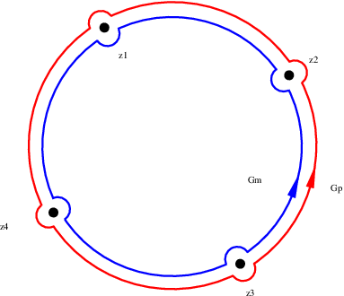
around contours Γ±\Gamma_{\pm} which are entirely contained in the regions |z2|>|z1||z_{2}|>|z_{1}| and |z2|<|z1||z_{2}|<|z_{1}| respectively, as depicted in Figure 1(a)(a),

{centering}
Refer to caption Refer to caption
(a)(a) (b)(b)
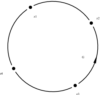
Figure 1: The black dots denote the poles of the projection kernels (4.5) at in​z1i^{n}z_{1} in the z2z_{2}-plane. Figure (a)(a) shows the (red) contour Γ+\Gamma_{+} for π+\pi_{+} which contains all four singularities and the (blue) contour Γ−\Gamma_{-} for π−\pi_{-} which goes around the origin but contains none of the singularities. Figure (b)(b) shows the contour for the RR-matrix, namely Γ={|z2|=|z1|}\Gamma=\{|z_{2}|=|z_{1}|\} with all four singularities cut out.

namely

(π±X)𝟏¯(z1)=±∮Γ±d​z22​π​i​z2ϕ(z2)⟨κ𝟏¯​𝟐¯(z1,z2),X𝟐¯(z2)⟩𝟐¯.(\pi_{\pm}X)_{{\bf\underline{1}}}(z_{1})=\pm\oint_{\Gamma_{\pm}}\frac{dz_{2}}{2\pi iz_{2}}\phi(z_{2})\langle\kappa_{{\bf\underline{1}}{\bf\underline{2}}}(z_{1},z_{2}),X_{{\bf\underline{2}}}(z_{2})\rangle_{{\bf\underline{2}}}. (4.6)

We can thus also write the action of (4.2) as a contour integral

(RX)𝟏¯(z1)=(∮Γ++∮Γ−)d​z22​π​i​z2ϕ(z2)⟨κ𝟏¯​𝟐¯(z1,z2),X𝟐¯(z2)⟩𝟐¯.(RX)_{{\bf\underline{1}}}(z_{1})=\left(\oint_{\Gamma_{+}}+\oint_{\Gamma_{-}}\right)\frac{dz_{2}}{2\pi iz_{2}}\phi(z_{2})\langle\kappa_{{\bf\underline{1}}{\bf\underline{2}}}(z_{1},z_{2}),X_{{\bf\underline{2}}}(z_{2})\rangle_{{\bf\underline{2}}}.

In the limit where the contours Γ±\Gamma_{\pm} converge to Γ≔{|z2|=|z1|}\Gamma\coloneqq\{|z_{2}|=|z_{1}|\}, the contributions from the small semi-circles around the singularities at in​z1i^{n}z_{1} cancel (since each contribute opposite half residues) and we are left with twice the principal value of the integral around Γ\Gamma, namely

(R​X)𝟏¯​(z1)=2​v.p.​∮Γd​z22​π​i​z2​ϕ​(z2)​⟨κ𝟏¯​𝟐¯​(z1,z2),X𝟐¯​(z2)⟩𝟐¯,(RX)_{{\bf\underline{1}}}(z_{1})=2\,\text{v.p.}\oint_{\Gamma}\frac{dz_{2}}{2\pi iz_{2}}\phi(z_{2})\langle\kappa_{{\bf\underline{1}}{\bf\underline{2}}}(z_{1},z_{2}),X_{{\bf\underline{2}}}(z_{2})\rangle_{{\bf\underline{2}}}, (4.7)

In conclusion the kernel of the RR-matrix admits the following expression,

R𝟏¯​𝟐¯​(z1,z2)=2​v.p.​∑j=03z1j​z24−j​C𝟏¯​𝟐¯(j​ 4−j)z24−z14​ϕ​(z2)−1,R_{{\bf\underline{1}}{\bf\underline{2}}}(z_{1},z_{2})=2\,\text{v.p.}\frac{\sum_{j=0}^{3}z_{1}^{j}z_{2}^{4-j}C^{(j\,4-j)}_{{\bf\underline{1}}{\bf\underline{2}}}}{z_{2}^{4}-z_{1}^{4}}\phi(z_{2})^{-1}, (4.8a)
where the principal value symbol is to be understood in the sense of the preceding integral (4.7), along the contour shown in Figure 1(b)(b). Likewise we obtain from (4.4), or more directly using R𝟏¯​𝟐¯∗=P⁡(R𝟏¯​𝟐¯)R^{\ast}_{{\bf\underline{1}}{\bf\underline{2}}}=P(R_{{\bf\underline{1}}{\bf\underline{2}}}) (see appendix A), an expression for the kernel of the adjoint R∗R^{\ast}, namely
R𝟏¯​𝟐¯∗​(z1,z2)=2​v.p.​∑j=03z14−j​z2j​C𝟏¯​𝟐¯(4−j​j)z14−z24​ϕ​(z1)−1.R^{\ast}_{{\bf\underline{1}}{\bf\underline{2}}}(z_{1},z_{2})=2\,\text{v.p.}\frac{\sum_{j=0}^{3}z_{1}^{4-j}z_{2}^{j}C^{(4-j\,j)}_{{\bf\underline{1}}{\bf\underline{2}}}}{z_{1}^{4}-z_{2}^{4}}\phi(z_{1})^{-1}. (4.8b)

Yang-Baxter equation.

It is straightforward to check, using the fact that ℒ​𝔤±⊂ℒ​𝔤\mathcal{L}\mathfrak{g}_{\pm}\subset\mathcal{L}\mathfrak{g} are Lie subalgebras, that (4.2) satisfies the modified classical Yang-Baxter equation (mCYBE),

[R​X,R​Y]−R⁡([R​X,Y]+[X,R​Y])=−[X,Y],∀X,Y∈ℒ​𝔤.[RX,RY]-R([RX,Y]+[X,RY])=-[X,Y],\qquad\forall X,Y\in\mathcal{L}\mathfrak{g}. (4.9)

Moreover, this is a sufficient condition for (4.1) to satisfy the Jacobi identity.

Taking the inner product with an arbitrary Z∈ℒ​𝔤Z\in\mathcal{L}\mathfrak{g}, its right hand side defines a 3-form on ℒ​𝔤\mathcal{L}\mathfrak{g}, namely ω^​(X,Y,Z)≔([X,Y],Z)ϕ\hat{\omega}(X,Y,Z)\coloneqq([X,Y],Z)_{\phi}. Let ω^𝟏¯​𝟐¯​𝟑¯\hat{\omega}_{{\bf\underline{1}}{\bf\underline{2}}{\bf\underline{3}}} denote its tensor kernel with respect to (3.5) which can be written explicitly as

ω^𝟏¯​𝟐¯​𝟑¯​(z1,z2,z3)≔ω𝟏¯​𝟐¯​𝟑¯​ϕ​(z1)−2​δ​(z1−z2)​δ​(z2−z3),\hat{\omega}_{{\bf\underline{1}}{\bf\underline{2}}{\bf\underline{3}}}(z_{1},z_{2},z_{3})\coloneqq\omega_{{\bf\underline{1}}{\bf\underline{2}}{\bf\underline{3}}}\,\phi(z_{1})^{-2}\delta(z_{1}-z_{2})\delta(z_{2}-z_{3}), (4.10)

where ω𝟏¯​𝟐¯​𝟑¯\omega_{{\bf\underline{1}}{\bf\underline{2}}{\bf\underline{3}}} is the tensor of the 3-form on 𝔤\mathfrak{g} given by ω⁡(x,y,z)≔⟨[x,y],z⟩\omega(x,y,z)\coloneqq\langle[x,y],z\rangle for x,y,z∈𝔤x,y,z\in\mathfrak{g}.

Using this to express the mCYBE (4.9) in tensor notation we obtain

[R𝟏¯​𝟐¯,R𝟏¯​𝟑¯]+[R𝟏¯​𝟐¯,R𝟐¯​𝟑¯]+[R𝟑¯​𝟐¯,R𝟏¯​𝟑¯]=−ω^𝟏¯​𝟐¯​𝟑¯.[R_{{\bf\underline{1}}{\bf\underline{2}}},R_{{\bf\underline{1}}{\bf\underline{3}}}]+[R_{{\bf\underline{1}}{\bf\underline{2}}},R_{{\bf\underline{2}}{\bf\underline{3}}}]+[R_{{\bf\underline{3}}{\bf\underline{2}}},R_{{\bf\underline{1}}{\bf\underline{3}}}]=-\hat{\omega}_{{\bf\underline{1}}{\bf\underline{2}}{\bf\underline{3}}}. (4.11)

Despite appearances, this is not quite the same as the usual modified classical Yang-Baxter equation on the rr-matrix in the Lie bialgebra setting, which we shall call the rrmCYBE,

[r𝟏𝟐¯,r𝟏𝟑¯]+[r𝟏𝟐¯,r𝟐𝟑¯]+[r𝟏𝟑¯,r𝟐𝟑¯]=−ω^𝟏¯​𝟐¯​𝟑¯.[r_{{\bf\underline{12}}},r_{{\bf\underline{13}}}]+[r_{{\bf\underline{12}}},r_{{\bf\underline{23}}}]+[r_{{\bf\underline{13}}},r_{{\bf\underline{23}}}]=-\hat{\omega}_{{\bf\underline{1}}{\bf\underline{2}}{\bf\underline{3}}}. (4.12)

The difference between (4.11) and (4.12) can be understood by recalling (see appendix A) that the kernel R𝟏𝟐¯∗R^{\ast}_{{\bf\underline{12}}} of R∗R^{\ast} was P⁡(R𝟏¯​𝟐¯)P(R_{{\bf\underline{1}}{\bf\underline{2}}}), in other words R𝟏𝟐¯∗=R𝟐𝟏¯R^{\ast}_{{\bf\underline{12}}}=R_{{\bf\underline{21}}}. Therefore rewriting (4.11) as

[R𝟏𝟐¯,R𝟏𝟑¯]+[R𝟏𝟐¯,R𝟐𝟑¯]+[R𝟏𝟑¯,(−R∗)𝟐𝟑¯]=−ω^𝟏¯​𝟐¯​𝟑¯[R_{{\bf\underline{12}}},R_{{\bf\underline{13}}}]+[R_{{\bf\underline{12}}},R_{{\bf\underline{23}}}]+[R_{{\bf\underline{13}}},(-R^{\ast})_{{\bf\underline{23}}}]=-\hat{\omega}_{{\bf\underline{1}}{\bf\underline{2}}{\bf\underline{3}}} (4.13)

it becomes clear that if R∗=−RR^{\ast}=-R then the RR-matrix satisfies the usual rrmCYBE. In fact one can show that when RR is assumed skew-symmetric, the RR-matrix construction yields a coboundary Lie bialgebra with RR as rr-matrix. Indeed, suppose 𝔥\mathfrak{h} is a coboundary Lie bialgebra with 1-cocycle δ:𝔥→𝔥∧𝔥\delta:\mathfrak{h}\rightarrow\mathfrak{h}\wedge\mathfrak{h} given by δ⁡(X)=12​[1⊗X+X⊗1,r]\delta(X)=\mbox{\small$\frac{1}{2}$}[1\otimes X+X\otimes 1,r], X∈𝔥X\in\mathfrak{h}. Its dual Lie bracket on 𝔥∗\mathfrak{h}^{\ast} then reads

[ξ,ξ′]∗=12​(a​d∗​r​ξ⋅ξ′+a​d∗​r∗​ξ′⋅ξ),∀ξ,ξ′∈𝔥∗.[\xi,\xi^{\prime}]_{\ast}=\mbox{\small$\frac{1}{2}$}\left(ad^{\ast}r\xi\cdot\xi^{\prime}+ad^{\ast}r^{\ast}\xi^{\prime}\cdot\xi\right),\qquad\forall\xi,\xi^{\prime}\in\mathfrak{h}^{\ast}.

Under the identification 𝔥∗≃𝔥\mathfrak{h}^{\ast}\simeq\mathfrak{h} and assuming r∗=−rr^{\ast}=-r, this is exactly of the form (4.1) with R=rR=r. Yet in the case at hand the RR-matrix is not skew-symmetric but instead satisfies (4.4), due to the twist in the inner product (3.5).

5 Centrally extended current algebra

Recall that the phase-space 𝒫\mathcal{P} is parametrised by a pair of fields in C∞​(S1,𝔤)C^{\infty}(S^{1},\mathfrak{g}), which is a particular realisation of the loop algebra over 𝔤\mathfrak{g}, the so-called current algebra. In the previous section we had considered a different kind of realisation, namely the twisted loop algebra ℒ​𝔤Ω\mathcal{L}\mathfrak{g}^{\mbox{\scriptsize$\Omega$}}, and equipped it with a Lie dialgebra structure. We can anticipate that studying the integrable structure of 𝒫\mathcal{P} will require working with a double loop algebra over 𝔤\mathfrak{g}, specifically the current algebra of ℒ​𝔤Ω\mathcal{L}\mathfrak{g}^{\mbox{\scriptsize$\Omega$}}.

In this section we show in fact that in order to obtain zero curvature equations – which constitute the main ingredient in any 22-d integrable field theory – the relevant algebra to consider is a central extension of the current algebra of ℒ​𝔤Ω\mathcal{L}\mathfrak{g}^{\mbox{\scriptsize$\Omega$}}.

Double loop algebra.

Consider the current algebra 𝔊≔C∞​(S1,ℒ​𝔤Ω)\mathfrak{G}\coloneqq C^{\infty}(S^{1},\mathcal{L}\mathfrak{g}^{\mbox{\scriptsize$\Omega$}}) of smooth loops in ℒ​𝔤Ω\mathcal{L}\mathfrak{g}^{\mbox{\scriptsize$\Omega$}}. Introducing the subalgebras 𝔊±≔C∞​(S1,ℒ​𝔤±Ω)\mathfrak{G}_{\pm}\coloneqq C^{\infty}(S^{1},\mathcal{L}\mathfrak{g}^{\mbox{\scriptsize$\Omega$}}_{\pm}), the decomposition (3.1) leads to

𝔊=𝔊+∔𝔊−.\mathfrak{G}=\mathfrak{G}_{+}\dotplus\mathfrak{G}_{-}. (5.1)

Let us also introduce the subalgebras 𝔊±⟂≔C∞​(S1,(ℒ​𝔤±Ω)⟂)\mathfrak{G}_{\pm}^{\perp}\coloneqq C^{\infty}(S^{1},(\mathcal{L}\mathfrak{g}^{\mbox{\scriptsize$\Omega$}}_{\pm})^{\perp}) corresponding to (3.6). We define a non-degenerate, invariant, bilinear form on 𝔊\mathfrak{G}, given for 𝔛,𝔜∈𝔊\mathfrak{X},\mathfrak{Y}\in\mathfrak{G} by

((𝔛,𝔜))ϕ≔∫S1d​σ​(𝔛⁡(σ),𝔜⁡(σ))ϕ.(\!(\mathfrak{X},\mathfrak{Y})\!)_{\phi}\coloneqq\int_{S^{1}}d\sigma(\mathfrak{X}(\sigma),\mathfrak{Y}(\sigma))_{\phi}. (5.2)

It gives an embedding of 𝔊\mathfrak{G} into its dual 𝔊′\mathfrak{G}^{\prime} whose image 𝔊∗⊂𝔊′\mathfrak{G}^{\ast}\subset\mathfrak{G}^{\prime} defines the smooth dual. Owing to the twist in the inner product, the smooth dual can be identified as

𝔊∗≃ϕ−1​𝔊≔{ϕ−1​𝔛|𝔛∈𝔊}⊂𝔊.\mathfrak{G}^{\ast}\simeq\phi^{-1}\mathfrak{G}\coloneqq\{\phi^{-1}\mathfrak{X}\,|\,\mathfrak{X}\in\mathfrak{G}\}\subset\mathfrak{G}. (5.3)

Central extension.

The current algebra 𝔊\mathfrak{G} admits an important central extension 𝔊^\hat{\mathfrak{G}} defined by the 2-cocycle

ω⁡(𝔛,𝔜)≔∫S1d​σ​(𝔛⁡(σ),∂σ𝔜⁡(σ))ϕ.\omega(\mathfrak{X},\mathfrak{Y})\coloneqq\int_{S^{1}}d\sigma(\mathfrak{X}(\sigma),\partial_{\sigma}\mathfrak{Y}(\sigma))_{\phi}. (5.4)

Specifically, 𝔊^\hat{\mathfrak{G}} is identified as a vector space with 𝔊⊕ℂ\mathfrak{G}\oplus\mathbb{C} and equipped with the Lie bracket

[(𝔛,a),(𝔜,b)]≔([𝔛,𝔜],ω⁡(𝔛,𝔜)).[(\mathfrak{X},a),(\mathfrak{Y},b)]\coloneqq([\mathfrak{X},\mathfrak{Y}],\omega(\mathfrak{X},\mathfrak{Y})). (5.5)

Notice that this definition doesn’t depend on aa or bb, corresponding to the fact that the extension is indeed central. Extending the inner product (5.2) to 𝔊^\hat{\mathfrak{G}} as

(((𝔛,a),(𝔜,b)))ϕ≔((𝔛,𝔜))ϕ+a​b,(\!((\mathfrak{X},a),(\mathfrak{Y},b))\!)_{\phi}\coloneqq(\!(\mathfrak{X},\mathfrak{Y})\!)_{\phi}+ab, (5.6)

one can identify the smooth dual 𝔊^∗\hat{\mathfrak{G}}^{\ast} with ϕ−1​𝔊⊕ℂ\phi^{-1}\mathfrak{G}\oplus\mathbb{C}.

Coadjoint action.

The point of centrally extending 𝔊\mathfrak{G} by (5.4) can be understood by looking at the coadjoint action of 𝔊^\hat{\mathfrak{G}} on 𝔊^∗\hat{\mathfrak{G}}^{\ast} defined as

((a​d∗​(𝔐,c)⋅(𝔛,a),(𝔜,b)))ϕ≔−(((𝔛,a),[(𝔐,c),(𝔜,b)]))ϕ.(\!(ad^{\ast}(\mathfrak{M},c)\cdot(\mathfrak{X},a),(\mathfrak{Y},b))\!)_{\phi}\coloneqq-(\!((\mathfrak{X},a),[(\mathfrak{M},c),(\mathfrak{Y},b)])\!)_{\phi}. (5.7)

Notice that the right hand side does not depend on c∈ℂc\in\mathbb{C}, using (5.5). In other words, the center of 𝔊^\hat{\mathfrak{G}} acts trivially in the coadjoint representation and (5.7) equally defines the coadjoint action of 𝔊\mathfrak{G} on 𝔊^∗\hat{\mathfrak{G}}^{\ast}. It is easy to show using (5.4), (5.5) and (5.6) that the latter takes the form

a​d∗​𝔐⋅(𝔛,a)=([𝔐,𝔛]+a​∂σ𝔐,0).ad^{\ast}\mathfrak{M}\cdot(\mathfrak{X},a)=([\mathfrak{M},\mathfrak{X}]+a\,\partial_{\sigma}\mathfrak{M},0).

Observing that a∈ℂa\in\mathbb{C} is invariant under this action we are free to set a=1a=1, which amounts to restricting attention to the subspace 𝔊^1∗=ϕ−1​𝔊⊕{1}⊂ϕ−1​𝔊⊕ℂ\hat{\mathfrak{G}}^{\ast}_{1}=\phi^{-1}\mathfrak{G}\oplus\{1\}\subset\phi^{-1}\mathfrak{G}\oplus\mathbb{C}, isomorphic to 𝔊∗\mathfrak{G}^{\ast}. Given any 𝔛∈𝔊\mathfrak{X}\in\mathfrak{G} (respectively 𝔛∈𝔊∗\mathfrak{X}\in\mathfrak{G}^{\ast}), we shall use the notation 𝔛^≔(𝔛,1)\hat{\mathfrak{X}}\coloneqq(\mathfrak{X},1) for the corresponding element in 𝔊^1\hat{\mathfrak{G}}_{1} (respectively 𝔊^1∗\hat{\mathfrak{G}}^{\ast}_{1}). Now although we can effectively ignore the central extension since 𝔊^1∗\hat{\mathfrak{G}}^{\ast}_{1} is isomorphic to 𝔊∗\mathfrak{G}^{\ast}, the extra σ\sigma-derivative term in the coadjoint action of 𝔊\mathfrak{G} on 𝔊^1∗\hat{\mathfrak{G}}^{\ast}_{1}, namely

a​d∗​𝔐⋅𝔛^=([𝔐,𝔛]+∂σ𝔐,0)ad^{\ast}\mathfrak{M}\cdot\hat{\mathfrak{X}}=([\mathfrak{M},\mathfrak{X}]+\partial_{\sigma}\mathfrak{M},0) (5.8)

and which is absent in the usual coadjoint action of 𝔊\mathfrak{G} on 𝔊∗\mathfrak{G}^{\ast}, is a remnant of this central extension.

The Kostant-Kirillov bracket.

The Lie algebra structure (5.5) on 𝔊^\hat{\mathfrak{G}} induces a natural Poisson structure on 𝔊^1∗\hat{\mathfrak{G}}^{\ast}_{1}. Given f∈C∞​(𝔊^∗)f\in C^{\infty}(\hat{\mathfrak{G}}^{\ast}) we define its derivative d^​f=(d​f,cf)∈𝔊^\hat{d}f=(df,c_{f})\in\hat{\mathfrak{G}} at (𝔏,a)∈𝔊^∗(\mathfrak{L},a)\in\hat{\mathfrak{G}}^{\ast} as

(((𝔛,b),d^​f))ϕ≔dd​t|t=0​f​((𝔏,a)+t⁡(𝔛,b)),∀(𝔛,b)∈𝔊^∗.(\!((\mathfrak{X},b),\hat{d}f)\!)_{\phi}\coloneqq\mbox{\small$\left.\frac{d}{dt}\right|_{t=0}$}f((\mathfrak{L},a)+t(\mathfrak{X},b)),\qquad\forall(\mathfrak{X},b)\in\hat{\mathfrak{G}}^{\ast}. (5.9)

Then for any two functions f,g∈C∞​(𝔊^1∗)f,g\in C^{\infty}(\hat{\mathfrak{G}}^{\ast}_{1}) we set

{f,g}​(𝔏^)≔((𝔏^,[d^​f,d^​g]))ϕ.\{f,g\}(\hat{\mathfrak{L}})\coloneqq(\!(\hat{\mathfrak{L}},[\hat{d}f,\hat{d}g])\!)_{\phi}. (5.10)

The anti-symmetry of (5.10) and the Jacobi identity follow from that of the Lie bracket on 𝔊^\hat{\mathfrak{G}}. This defines the Kostant-Kirillov bracket, making 𝔊^1∗\hat{\mathfrak{G}}^{\ast}_{1} into a Poisson manifold. Although the Poisson bracket (5.10) is very natural indeed, it is important to note that it is degenerate. Its kernel is easily shown to coincide with the set ℐ⁡(𝔊^1∗)⊂C∞​(𝔊^1∗)\mathcal{I}(\hat{\mathfrak{G}}^{\ast}_{1})\subset C^{\infty}(\hat{\mathfrak{G}}^{\ast}_{1}) of coadjoint invariant functions on 𝔊^1∗\hat{\mathfrak{G}}^{\ast}_{1}, which itself is characterised by

f∈ℐ(𝔊^1∗)⟺ad∗df⋅𝔏^=0,∀𝔏^∈𝔊^1∗.f\in\mathcal{I}(\hat{\mathfrak{G}}^{\ast}_{1})\quad\Longleftrightarrow\quad ad^{\ast}df\cdot\hat{\mathfrak{L}}=0,\;\forall\hat{\mathfrak{L}}\in\hat{\mathfrak{G}}^{\ast}_{1}. (5.11)

Now consider the simplest type of function on 𝔊^1∗\hat{\mathfrak{G}}^{\ast}_{1}, namely a linear one. It can be specified by an element 𝔛^∈(𝔊^1∗)∗≃𝔊^1\hat{\mathfrak{X}}\in(\hat{\mathfrak{G}}^{\ast}_{1})^{\ast}\simeq\hat{\mathfrak{G}}_{1} and is given explicitly as 𝔛^:𝔏^↦((𝔏^,𝔛^))ϕ\hat{\mathfrak{X}}:\hat{\mathfrak{L}}\mapsto(\!(\hat{\mathfrak{L}},\hat{\mathfrak{X}})\!)_{\phi}. From the definition (5.9) we find d^​𝔛^=𝔛^\hat{d}\hat{\mathfrak{X}}=\hat{\mathfrak{X}}. Its evolution under the flow ∂t≔{⋅,h}\partial_{t}\coloneqq\{\cdot,h\} corresponding to some h∈C∞​(𝔊^1∗)h\in C^{\infty}(\hat{\mathfrak{G}}^{\ast}_{1}) reads

∂t((𝔏^,𝔛^))ϕ={𝔛^,h}​(𝔏^)=((a​d∗​d​h⋅𝔏^,𝔛^))ϕ.\partial_{t}(\!(\hat{\mathfrak{L}},\hat{\mathfrak{X}})\!)_{\phi}=\{\hat{\mathfrak{X}},h\}(\hat{\mathfrak{L}})=(\!(ad^{\ast}dh\cdot\hat{\mathfrak{L}},\hat{\mathfrak{X}})\!)_{\phi}.

In other words, the flow of any h∈C∞​(𝔊^1∗)h\in C^{\infty}(\hat{\mathfrak{G}}^{\ast}_{1}) under the Kostant-Kirillov bracket (5.10) is tangent to the coadjoint orbit of 𝔊\mathfrak{G} in 𝔊^1∗\hat{\mathfrak{G}}^{\ast}_{1} since

∂t𝔏^=a​d∗​d​h⋅𝔏^.\partial_{t}\hat{\mathfrak{L}}=ad^{\ast}dh\cdot\hat{\mathfrak{L}}. (5.12)

Making use of (5.8) this takes the form of a zero curvature equation,

∂t𝔏−∂σ𝔑=[𝔑,𝔏],where𝔑=d​h.\partial_{t}\mathfrak{L}-\partial_{\sigma}\mathfrak{N}=[\mathfrak{N},\mathfrak{L}],\qquad\text{where}\quad\mathfrak{N}=dh. (5.13)

One might hastily conclude that the space 𝔊^1∗\hat{\mathfrak{G}}^{\ast}_{1} provides a natural setting for describing integrable 22-d field theories. The problem is that any function h∈C∞​(𝔊^1∗)h\in C^{\infty}(\hat{\mathfrak{G}}^{\ast}_{1}) generates a zero curvature flow, which is unlikely to yield a valid setting for non-trivial examples of integrable 22-d field theories. Indeed, suppose that f∈C∞​(𝔊^1∗)f\in C^{\infty}(\hat{\mathfrak{G}}^{\ast}_{1}) is invariant under all these flows, that is 0=∂tf={f,h}0=\partial_{t}f=\{f,h\}, then necessarily it must lie in the kernel of the Kostant-Kirillov bracket (5.10). In other words, such an ff generates a trivial flow on 𝔊^1∗\hat{\mathfrak{G}}^{\ast}_{1}.

6 Kostant-Kirillov RR-bracket

The 𝑹\bm{R}-bracket.

In order to circumvent this difficulty one is led to the introduction of a second Poisson structure on 𝔊^1∗\hat{\mathfrak{G}}^{\ast}_{1}, such that the Casimirs of (5.10) are not in its center. One way to achieve this is to endow 𝔊^\hat{\mathfrak{G}} itself with a second Lie bracket distinct from the original one. In the RR-matrix approach this second bracket is constructed from a given linear operator R∈End ​𝔊^R\in\text{End }\hat{\mathfrak{G}}. Starting from R∈End​ℒ​𝔤ΩR\in\text{End}\;\mathcal{L}\mathfrak{g}^{\mbox{\scriptsize$\Omega$}} given in (4.2) we can extend it to End​𝔊\text{End}\;\mathfrak{G} trivially by setting (R​𝔛)​(σ)=R​(𝔛​(σ))(R\mathfrak{X})(\sigma)=R(\mathfrak{X}(\sigma)), which allows us to define the RR-bracket on 𝔊\mathfrak{G} by the usual formula

[𝔛,𝔜]R≔12​([R​𝔛,𝔜]+[𝔛,R​𝔜]).[\mathfrak{X},\mathfrak{Y}]_{R}\coloneqq\mbox{\small$\frac{1}{2}$}\left([R\mathfrak{X},\mathfrak{Y}]+[\mathfrak{X},R\mathfrak{Y}]\right). (6.1)

The anti-symmetry is evident and the Jacobi identity holds by virtue of the mCYBE (4.9). One sometimes denotes vector space 𝔊\mathfrak{G} equipped with the RR-bracket (6.1) as 𝔊R\mathfrak{G}_{R}, to distinguish it from the Lie algebra 𝔊\mathfrak{G} with the original Lie bracket.

We then further extend the RR-matrix to End​𝔊^\text{End}\,\hat{\mathfrak{G}} simply as R⁡(𝔛,c)=(R​𝔛,c)R(\mathfrak{X},c)=(R\mathfrak{X},c). The corresponding RR-bracket on 𝔊^\hat{\mathfrak{G}} defined by the analog of (6.1) evaluates to

[(𝔛,a),(𝔜,b)]R≔12​([R⁡(𝔛,a),(𝔜,b)]+[(𝔛,a),R⁡(𝔜,b)])=([𝔛,𝔜]R,ωR​(𝔛,𝔜)),[(\mathfrak{X},a),(\mathfrak{Y},b)]_{R}\coloneqq\mbox{\small$\frac{1}{2}$}\left([R(\mathfrak{X},a),(\mathfrak{Y},b)]+[(\mathfrak{X},a),R(\mathfrak{Y},b)]\right)=([\mathfrak{X},\mathfrak{Y}]_{R},\omega_{R}(\mathfrak{X},\mathfrak{Y})), (6.2)

where ωR​(𝔛,𝔜)≔12​(ω⁡(R​𝔛,𝔜)+ω⁡(𝔛,R​𝔜))\omega_{R}(\mathfrak{X},\mathfrak{Y})\coloneqq\mbox{\small$\frac{1}{2}$}\left(\omega(R\mathfrak{X},\mathfrak{Y})+\omega(\mathfrak{X},R\mathfrak{Y})\right). Define the Kostant-Kirillov RR-bracket on 𝔊^1∗\hat{\mathfrak{G}}^{\ast}_{1} as

12​{f,g}R​(𝔏^)≔((𝔏^,[d^​f,d^​g]R))ϕ.\mbox{\small$\frac{1}{2}$}\{f,g\}_{R}(\hat{\mathfrak{L}})\coloneqq(\!(\hat{\mathfrak{L}},[\hat{d}f,\hat{d}g]_{R})\!)_{\phi}. (6.3)

Here the factor of a half was introduced for convenience. Making use of (6.2) this can be evaluated explicitly to give

{f,g}R​(𝔏^)=−((,,,))ϕ,\{f,g\}_{R}(\hat{\mathfrak{L}})=-(\!(df,\mathcal{H}_{R}(\mathfrak{L})\cdot dg)\!)_{\phi}, (6.4a)
where the Poisson operator ℋR​(𝔏)\mathcal{H}_{R}(\mathfrak{L}) is given by the skew-selfadjoint operator
ℋR(𝔏)≔ad𝔏∘R+R∗∘ad𝔏−(R+R∗)∂σ.\mathcal{H}_{R}(\mathfrak{L})\coloneqq ad\;\mathfrak{L}\circ R+R^{\ast}\circ ad\;\mathfrak{L}-(R+R^{\ast})\partial_{\sigma}. (6.4b)

The presence of the term in ∂σ\partial_{\sigma} stems once again from working with the central extension. Making use of the tensor notation in appendix A to rewrite the bracket (6.4) yields

{f,g}R​(𝔏^)=∫S1d​σ​(([R𝟏¯​𝟐¯,𝔏⊗𝟏]−[R𝟏¯​𝟐¯∗,𝟏⊗𝔏],𝑑f⊗𝑑g)ϕ+(R𝟏¯​𝟐¯+R𝟏¯​𝟐¯∗,𝑑f⊗∂σ𝑑g)ϕ).\{f,g\}_{R}(\hat{\mathfrak{L}})=\int_{S^{1}}d\sigma\left(([R_{{\bf\underline{1}}{\bf\underline{2}}},\mathfrak{L}\otimes{\bf 1}]-[R^{\ast}_{{\bf\underline{1}}{\bf\underline{2}}},{\bf 1}\otimes\mathfrak{L}],df\otimes dg)_{\phi}+(R_{{\bf\underline{1}}{\bf\underline{2}}}+R^{\ast}_{{\bf\underline{1}}{\bf\underline{2}}},df\otimes\partial_{\sigma}dg)_{\phi}\right). (6.5)

The r/sr/s-formalism.

The bracket (6.5) is usually written for linear functions f,g∈C∞​(𝔊^1∗)f,g\in C^{\infty}(\hat{\mathfrak{G}}^{\ast}_{1}). So let X,Y∈ℒ​𝔤ΩX,Y\in\mathcal{L}\mathfrak{g}^{\mbox{\scriptsize$\Omega$}} and set 𝔛=X⋅δσ1\mathfrak{X}=X\cdot\delta_{\sigma_{1}}, 𝔜=Y⋅δσ2\mathfrak{Y}=Y\cdot\delta_{\sigma_{2}} where δσ\delta_{\sigma} denotes the Dirac δ\delta-function based at the point σ∈S1\sigma\in S^{1}. With these definitions we choose the linear functions

f:𝔏^↦((𝔏^,(𝔛,0)))ϕ=(𝔏⁡(σ1),X)ϕ,g:𝔏^↦((𝔏^,(𝔜,0)))ϕ=(𝔏⁡(σ2),Y)ϕ.f:\hat{\mathfrak{L}}\mapsto(\!(\hat{\mathfrak{L}},(\mathfrak{X},0))\!)_{\phi}=(\mathfrak{L}(\sigma_{1}),X)_{\phi},\qquad g:\hat{\mathfrak{L}}\mapsto(\!(\hat{\mathfrak{L}},(\mathfrak{Y},0))\!)_{\phi}=(\mathfrak{L}(\sigma_{2}),Y)_{\phi}.

Now by abuse of notation the left hand side of (6.5) is usually written replacing the functions f,gf,g by their values at 𝔏^\hat{\mathfrak{L}}, or equivalently {f,g}R​(𝔏^)=({𝔏​,⊗​𝔏}R,X⊗Y)ϕ\{f,g\}_{R}(\hat{\mathfrak{L}})=(\{\mathfrak{L}\overset{\otimes}{,}\mathfrak{L}\}_{R},X\otimes Y)_{\phi} where it is understood that the first and second tensor factors depend on σ1\sigma_{1} and σ2\sigma_{2} respectively. By evaluating the right hand side of (6.5), using the standard notation 𝔏𝟏¯=𝔏⊗𝟏\mathfrak{L}_{{\bf\underline{1}}}=\mathfrak{L}\otimes{\bf 1}, 𝔏𝟐¯=𝟏⊗𝔏\mathfrak{L}_{{\bf\underline{2}}}={\bf 1}\otimes\mathfrak{L} for tensor products and the fact that X,Y∈ℒ​𝔤ΩX,Y\in\mathcal{L}\mathfrak{g}^{\mbox{\scriptsize$\Omega$}} are arbitrary, we obtain

{𝔏𝟏¯,𝔏𝟐¯}R=[R𝟏¯​𝟐¯,𝔏𝟏¯]​δσ1​σ2−[R𝟏¯​𝟐¯∗,𝔏𝟐¯]​δσ1​σ2+(R𝟏¯​𝟐¯+R𝟏¯​𝟐¯∗)​δσ1​σ2′,\{\mathfrak{L}_{{\bf\underline{1}}},\mathfrak{L}_{{\bf\underline{2}}}\}_{R}=[R_{{\bf\underline{1}}{\bf\underline{2}}},\mathfrak{L}_{{\bf\underline{1}}}]\delta_{\sigma_{1}\sigma_{2}}-[R^{\ast}_{{\bf\underline{1}}{\bf\underline{2}}},\mathfrak{L}_{{\bf\underline{2}}}]\delta_{\sigma_{1}\sigma_{2}}+(R_{{\bf\underline{1}}{\bf\underline{2}}}+R^{\ast}_{{\bf\underline{1}}{\bf\underline{2}}})\delta^{\prime}_{\sigma_{1}\sigma_{2}}, (6.6)

where δσ1​σ2=δσ2​(σ1)\delta_{\sigma_{1}\sigma_{2}}=\delta_{\sigma_{2}}(\sigma_{1}) and δσ1​σ2′=δσ2′​(σ1)\delta^{\prime}_{\sigma_{1}\sigma_{2}}=\delta^{\prime}_{\sigma_{2}}(\sigma_{1}). Comparing this bracket to the standard r/sr/s-algebra [11] we see that they are equivalent if we make the following identifications

r≔12​(R−R∗),s≔−12​(R+R∗).r\coloneqq\frac{1}{2}(R-R^{\ast}),\qquad s\coloneqq-\frac{1}{2}(R+R^{\ast}). (6.7)

In other words the ss-matrix is nothing but (minus) the symmetric part of the RR-matrix whereas the rr-matrix corresponds to its skew-symmetric part [27]. In particular the condition s=0s=0 for ultralocality is equivalent to the skew-symmetry R∗=−RR^{\ast}=-R of the RR-matrix. The non-ultralocality of the supercoset σ\sigma-model can therefore be attributed to the twisted inner product (3.5), which results in the non skew-symmetric condition (4.4). Substituting the kernels (4.8) of RR and R∗R^{\ast} into the definitions (6.7) we obtain the following kernels for the r/sr/s-matrices,

r𝟏¯​𝟐¯​(z1,z2)=v.p.\displaystyle r_{{\bf\underline{1}}{\bf\underline{2}}}(z_{1},z_{2})=\text{v.p.} 1z24−z14​[∑j=03z14−j​z2j​C𝟏¯​𝟐¯(4−j​j)​ϕ​(z1)−1+∑j=03z1j​z24−j​C𝟏¯​𝟐¯(j​ 4−j)​ϕ​(z2)−1],\displaystyle\frac{1}{z_{2}^{4}-z_{1}^{4}}\left[\sum_{j=0}^{3}z_{1}^{4-j}z_{2}^{j}C^{(4-j\,j)}_{{\bf\underline{1}}{\bf\underline{2}}}\phi(z_{1})^{-1}+\sum_{j=0}^{3}z_{1}^{j}z_{2}^{4-j}C^{(j\,4-j)}_{{\bf\underline{1}}{\bf\underline{2}}}\phi(z_{2})^{-1}\right], (6.8a)
s𝟏¯​𝟐¯​(z1,z2)=\displaystyle s_{{\bf\underline{1}}{\bf\underline{2}}}(z_{1},z_{2})=\, 1z24−z14​[∑j=03z14−j​z2j​C𝟏¯​𝟐¯(4−j​j)​ϕ​(z1)−1−∑j=03z1j​z24−j​C𝟏¯​𝟐¯(j​ 4−j)​ϕ​(z2)−1].\displaystyle\frac{1}{z_{2}^{4}-z_{1}^{4}}\left[\sum_{j=0}^{3}z_{1}^{4-j}z_{2}^{j}C^{(4-j\,j)}_{{\bf\underline{1}}{\bf\underline{2}}}\phi(z_{1})^{-1}-\sum_{j=0}^{3}z_{1}^{j}z_{2}^{4-j}C^{(j\,4-j)}_{{\bf\underline{1}}{\bf\underline{2}}}\phi(z_{2})^{-1}\right]. (6.8b)

Note that the expression (6.8b) is regular as z1→in​z2z_{1}\rightarrow i^{n}z_{2} so the principal value is not needed for s𝟏¯​𝟐¯s_{{\bf\underline{1}}{\bf\underline{2}}}. If we neglect contact terms by omitting the principal value in r𝟏¯​𝟐¯r_{{\bf\underline{1}}{\bf\underline{2}}} as well then these expressions are exactly the r/sr/s-matrices of [16], up to an irrelevant overall factor of 44.

Yang-Baxter equation.

The mCYBE (4.13) can also be rewritten in the equivalent form

[R𝟏𝟐¯,(−R∗)𝟏𝟑¯]+[(−R∗)𝟏𝟐¯,(−R∗)𝟐𝟑¯]+[(−R∗)𝟏𝟑¯,(−R∗)𝟐𝟑¯]=−ω^𝟏¯​𝟐¯​𝟑¯.[R_{{\bf\underline{12}}},(-R^{\ast})_{{\bf\underline{13}}}]+[(-R^{\ast})_{{\bf\underline{12}}},(-R^{\ast})_{{\bf\underline{23}}}]+[(-R^{\ast})_{{\bf\underline{13}}},(-R^{\ast})_{{\bf\underline{23}}}]=-\hat{\omega}_{{\bf\underline{1}}{\bf\underline{2}}{\bf\underline{3}}}. (6.9)

Now using the definition (6.7) of the r/sr/s-matrices we have R=r−sR=r-s and −R∗=r+s-R^{\ast}=r+s, and making use of (4.10) for the right hand side we can rewrite (6.9) in full as follows,

[r𝟏𝟑¯​(z1,z3)+s𝟏𝟑¯​(z1,z3),r𝟏𝟐¯​(z1,z2)−s𝟏𝟐¯​(z1,z2)]+[r𝟐𝟑¯​(z2,z3)+s𝟐𝟑¯​(z2,z3),r𝟏𝟐¯​(z1,z2)+s𝟏𝟐¯​(z1,z2)]+[r𝟐𝟑¯​(z2,z3)+s𝟐𝟑¯​(z2,z3),r𝟏𝟑¯​(z1,z3)+s𝟏𝟑¯​(z1,z3)]=−ω𝟏¯​𝟐¯​𝟑¯​ϕ​(z1)−2​δ​(z1−z2)​δ​(z2−z3).[r_{{\bf\underline{13}}}(z_{1},z_{3})+s_{{\bf\underline{13}}}(z_{1},z_{3}),r_{{\bf\underline{12}}}(z_{1},z_{2})-s_{{\bf\underline{12}}}(z_{1},z_{2})]+[r_{{\bf\underline{23}}}(z_{2},z_{3})+s_{{\bf\underline{23}}}(z_{2},z_{3}),r_{{\bf\underline{12}}}(z_{1},z_{2})+s_{{\bf\underline{12}}}(z_{1},z_{2})]\\ +[r_{{\bf\underline{23}}}(z_{2},z_{3})+s_{{\bf\underline{23}}}(z_{2},z_{3}),r_{{\bf\underline{13}}}(z_{1},z_{3})+s_{{\bf\underline{13}}}(z_{1},z_{3})]=-\omega_{{\bf\underline{1}}{\bf\underline{2}}{\bf\underline{3}}}\,\phi(z_{1})^{-2}\delta(z_{1}-z_{2})\delta(z_{2}-z_{3}).

If we neglect the contact terms once more then the δ\delta-functions on the right hand side disappear, and we are left precisely with the so-called “extended” classical Yang-Baxter equation satisfied by the pair of matrices rr and ss [11]. We see that the correct form of this equation, including contact terms, is simply the mCYBE for a non skew-symmetric RR-matrix.

7 Lax matrix and coadjoint orbit

Coadjoint RR-action.

In much the same way as the Kostant-Kirillov bracket (5.10) generated flows (5.12) along the coadjoint orbit of 𝔊\mathfrak{G} in 𝔊^1∗\hat{\mathfrak{G}}^{\ast}_{1}, the second Poisson bracket (6.3) will also generate flows along a different kind of coadjoint orbit in 𝔊^1∗\hat{\mathfrak{G}}^{\ast}_{1}.

To see this, define the coadjoint action a​dR∗ad_{R}^{\ast} of 𝔊^\hat{\mathfrak{G}} on 𝔊^∗\hat{\mathfrak{G}}^{\ast} corresponding to the RR-bracket (6.2) on 𝔊^\hat{\mathfrak{G}}, in analogy with the definition (5.7) of the coadjoint action a​d∗ad^{\ast} for the Lie bracket,

((a​dR∗​(𝔐,c)⋅(𝔛,a),(𝔜,b)))ϕ≔−(((𝔛,a),[(𝔐,c),(𝔜,b)]R))ϕ.(\!(ad_{R}^{\ast}(\mathfrak{M},c)\cdot(\mathfrak{X},a),(\mathfrak{Y},b))\!)_{\phi}\coloneqq-(\!((\mathfrak{X},a),[(\mathfrak{M},c),(\mathfrak{Y},b)]_{R})\!)_{\phi}. (7.1)

As was the case for the coadjoint action (5.7), the right hand side is independent of c∈ℂc\in\mathbb{C}, which follows from (6.2). The center of 𝔊^\hat{\mathfrak{G}} thus also acts trivially under a​dR∗ad_{R}^{\ast}, and hence the same expression (7.1) also defines the a​dR∗ad_{R}^{\ast}-action of 𝔊\mathfrak{G} on 𝔊^∗\hat{\mathfrak{G}}^{\ast}, i.e. the coadjoint action of 𝔊R\mathfrak{G}_{R} on 𝔊^∗\hat{\mathfrak{G}}^{\ast}.

Consider again the linear function given by 𝔛^∈𝔊^1\hat{\mathfrak{X}}\in\hat{\mathfrak{G}}_{1}. Its evolution under the flow ∂τ≔{⋅,h}R\partial_{\tau}\coloneqq\{\cdot,h\}_{R} generated by any h∈C∞​(𝔊^1∗)h\in C^{\infty}(\hat{\mathfrak{G}}^{\ast}_{1}) reads ∂τ((𝔏^,𝔛^))ϕ={𝔛^,h}R​(𝔏^)=2​((a​dR∗​d​h⋅𝔏^,𝔛^))ϕ\partial_{\tau}(\!(\hat{\mathfrak{L}},\hat{\mathfrak{X}})\!)_{\phi}=\{\hat{\mathfrak{X}},h\}_{R}(\hat{\mathfrak{L}})=2(\!(ad_{R}^{\ast}dh\cdot\hat{\mathfrak{L}},\hat{\mathfrak{X}})\!)_{\phi}, which we can write simply as

∂τ𝔏^=2​a​dR∗​d​h⋅𝔏^.\partial_{\tau}\hat{\mathfrak{L}}=2\,ad_{R}^{\ast}dh\cdot\hat{\mathfrak{L}}. (7.2)

In other words, the flow of any h∈C∞​(𝔊^1∗)h\in C^{\infty}(\hat{\mathfrak{G}}^{\ast}_{1}) with respect to the Poisson bracket (6.4) is tangent to the coadjoint orbit of 𝔊R\mathfrak{G}_{R} in 𝔊^1∗\hat{\mathfrak{G}}^{\ast}_{1}.

Lemma 7.1.

The a​d∗ad^{\ast}- and a​dR∗ad_{R}^{\ast}-actions of 𝔊\mathfrak{G} on 𝔊^∗\hat{\mathfrak{G}}^{\ast} are related as

a​dR∗​𝔛=12​a​d∗​(R​𝔛)+12​R∗∘a​d∗​𝔛,𝔛∈𝔊.ad_{R}^{\ast}\mathfrak{X}=\mbox{\small$\frac{1}{2}$}ad^{\ast}(R\,\mathfrak{X})+\mbox{\small$\frac{1}{2}$}R^{\ast}\circ ad^{\ast}\mathfrak{X},\qquad\mathfrak{X}\in\mathfrak{G}. (7.3)
Proof.

This follows from the definitions (5.7), (6.2) and (7.1). ∎

Zero-curvature equation.

The following important theorem provides a justification for having introduced the new Poisson bracket (6.3) based on the RR-bracket.

Theorem 7.2.

The set ℐ⁡(𝔊^1∗)\mathcal{I}(\hat{\mathfrak{G}}^{\ast}_{1}) of Casimirs for (5.10) are in involution with respect to (6.3) and the flow ∂τ≔{⋅,h}R\partial_{\tau}\coloneqq\{\cdot,h\}_{R} generated by any h∈ℐ⁡(𝔊^1∗)h\in\mathcal{I}(\hat{\mathfrak{G}}^{\ast}_{1}) satisfies the zero curvature equation

∂τ𝔏−∂σ𝔐=[𝔐,𝔏],where𝔐=R⁡(d​h).\partial_{\tau}\mathfrak{L}-\partial_{\sigma}\mathfrak{M}=[\mathfrak{M},\mathfrak{L}],\qquad\text{where}\quad\mathfrak{M}=R(dh). (7.4)
Proof.

Let f,g∈ℐ⁡(𝔊^1∗)f,g\in\mathcal{I}(\hat{\mathfrak{G}}^{\ast}_{1}) be Casimirs of (5.10). Using (7.3), or directly from the definition (6.2) of the RR-bracket one can show that

{f,g}R​(𝔏^)=((a​d∗​d​g⋅𝔏^,R⁡(d^​f)))ϕ−((a​d∗​d​f⋅𝔏^,R⁡(d^​g)))ϕ.\{f,g\}_{R}(\hat{\mathfrak{L}})=(\!(ad^{\ast}dg\cdot\hat{\mathfrak{L}},R(\hat{d}f))\!)_{\phi}-(\!(ad^{\ast}df\cdot\hat{\mathfrak{L}},R(\hat{d}g))\!)_{\phi}.

But the property (5.11) implies that a​d∗​d​f⋅𝔏^=a​d∗​d​g⋅𝔏^=0ad^{\ast}df\cdot\hat{\mathfrak{L}}=ad^{\ast}dg\cdot\hat{\mathfrak{L}}=0 and hence {f,g}R=0\{f,g\}_{R}=0.

Now making use of (7.3) to rewrite equation (7.2) yields

∂τ𝔏^=a​d∗​R​(d​h)⋅𝔏^+R∗∘a​d∗​d​h⋅𝔏^.\partial_{\tau}\hat{\mathfrak{L}}=ad^{\ast}R(dh)\cdot\hat{\mathfrak{L}}+R^{\ast}\circ ad^{\ast}dh\cdot\hat{\mathfrak{L}}.

Since h∈ℐ⁡(𝔊^1∗)h\in\mathcal{I}(\hat{\mathfrak{G}}^{\ast}_{1}) the last term vanishes by (5.11) and using (5.8) we obtain (7.4). ∎

Notice that the flow ∂τ\partial_{\tau} not only lies in the coadjoint orbit of 𝔊R\mathfrak{G}_{R} in 𝔊^1∗\hat{\mathfrak{G}}^{\ast}_{1}, from its definition (7.2), but it also lies in the coadjoint orbit of 𝔊\mathfrak{G} in 𝔊^1∗\hat{\mathfrak{G}}^{\ast}_{1} from the fact that ∂τ𝔏^=a​d∗​R​(d​h)⋅𝔏^\partial_{\tau}\hat{\mathfrak{L}}=ad^{\ast}R(dh)\cdot\hat{\mathfrak{L}}.

Although theorem 7.2 is quite general, it is also possible to generate zero curvature equations from functions which are not in ℐ⁡(𝔊^1∗)\mathcal{I}(\hat{\mathfrak{G}}^{\ast}_{1}). Indeed, this was the case for the zero curvature equation obtained in [15] which is given by the following

Lemma 7.3.

Let P−:𝔏^↦−14​((𝔏^,𝔏^))ϕP_{-}:\hat{\mathfrak{L}}\mapsto-\mbox{\small$\frac{1}{4}$}(\!(\hat{\mathfrak{L}},\hat{\mathfrak{L}})\!)_{\phi} and ∂−≔{⋅,P−}R\partial_{-}\coloneqq\{\cdot,P_{-}\}_{R}. Although P−∉ℐ⁡(𝔊^1∗)P_{-}\not\in\mathcal{I}(\hat{\mathfrak{G}}^{\ast}_{1}) we still have,

∂−𝔏−∂σ𝔏−=[𝔏−,𝔏],where𝔏−=π−​𝔏.\partial_{-}\mathfrak{L}-\partial_{\sigma}\mathfrak{L}_{-}=[\mathfrak{L}_{-},\mathfrak{L}],\qquad\text{where}\quad\mathfrak{L}_{-}=\pi_{-}\mathfrak{L}.
Proof.

From the definition (5.9) we get d​P−=−12​𝔏dP_{-}=-\mbox{\small$\frac{1}{2}$}\mathfrak{L}. Note also that due to the special form (3.9) of the Lax matrix 𝔏\mathfrak{L} and the expression (4.4) for the adjoint R∗R^{\ast} we have the relation R∗​𝔏=−𝔏R^{\ast}\mathfrak{L}=-\mathfrak{L}. Using all this we find R∗∘a​d∗​d​P−⋅𝔏^=12​(∂σ𝔏,0)R^{\ast}\circ ad^{\ast}dP_{-}\cdot\hat{\mathfrak{L}}=\mbox{\small$\frac{1}{2}$}(\partial_{\sigma}\mathfrak{L},0). If P−P_{-} were in ℐ⁡(𝔊^1∗)\mathcal{I}(\hat{\mathfrak{G}}^{\ast}_{1}) this would vanish. Nevertheless, the coadjoint RR-action a​dR∗​d​P−⋅𝔏^=([π−​𝔏,𝔏]+∂σ(π−​𝔏),0)ad_{R}^{\ast}dP_{-}\cdot\hat{\mathfrak{L}}=([\pi_{-}\mathfrak{L},\mathfrak{L}]+\partial_{\sigma}(\pi_{-}\mathfrak{L}),0) still takes a zero curvature form. ∎

Lax matrix.

The upshot of theorem 7.2 is the existence of integrable flows on (𝔊^1∗,{⋅,⋅}R)(\hat{\mathfrak{G}}^{\ast}_{1},\{\cdot,\cdot\}_{R}). Yet we are interested in the Hamiltonian dynamics of the supercoset σ\sigma-model which takes place on the phase-space (𝒫,{⋅,⋅})(\mathcal{P},\{\cdot,\cdot\}) defined in [15] (see section 2). The respective flows of the two systems can be related provided we have a Poisson map

𝔏^:(𝒫,{⋅,⋅})⟶(𝔊^1∗,{⋅,⋅}R),\hat{\mathfrak{L}}:(\mathcal{P},\{\cdot,\cdot\})\longrightarrow(\hat{\mathfrak{G}}^{\ast}_{1},\{\cdot,\cdot\}_{R}), (7.5)

meaning that {𝔏^∗​f,𝔏^∗​g}=𝔏^∗​{f,g}R\{\hat{\mathfrak{L}}^{\ast}f,\hat{\mathfrak{L}}^{\ast}g\}=\hat{\mathfrak{L}}^{\ast}\{f,g\}_{R} for any f,g∈C∞​(𝔊^1∗)f,g\in C^{\infty}(\hat{\mathfrak{G}}^{\ast}_{1}). Indeed, the pullback by such a map of the flows on 𝔊^1∗\hat{\mathfrak{G}}^{\ast}_{1} then correspond exactly to the dynamical flows on 𝒫\mathcal{P}. Note that once (7.5) has been specified one can equally work at the level of 𝔊^1∗\hat{\mathfrak{G}}^{\ast}_{1}.

The existence of such a Poisson map follows from the results of [15, 16] which we summarise in two propositions. Recall from section 3 that the Lax matrix 𝔏\mathfrak{L}, defined by (3.9), takes values in the smooth dual (ℒ​𝔤−Ω)∗≃ϕ−1​(ℒ​𝔤+Ω)⟂(\mathcal{L}\mathfrak{g}^{\mbox{\scriptsize$\Omega$}}_{-})^{\ast}\simeq\phi^{-1}(\mathcal{L}\mathfrak{g}^{\mbox{\scriptsize$\Omega$}}_{+})^{\perp}. The following proposition shows that both this statement and the form (3.9) of the Lax matrix 𝔏\mathfrak{L} are invariant under the flows of theorem 7.2.

Proposition 7.4.

The Lax matrix 𝔏^=(𝔏,1)\hat{\mathfrak{L}}=(\mathfrak{L},1) of the supercoset σ\sigma-model belongs to the coadjoint orbit 𝔊^σ∗\hat{\mathfrak{G}}^{\ast}_{\sigma} of 𝔊R\mathfrak{G}_{R} inside 𝔊^−∗≃ϕ−1​𝔊+⟂⊕{1}⊂𝔊^1∗\hat{\mathfrak{G}}^{\ast}_{-}\simeq\phi^{-1}\mathfrak{G}_{+}^{\perp}\oplus\{1\}\subset\hat{\mathfrak{G}}^{\ast}_{1} defined by 𝔏\mathfrak{L} having the explicit form

𝔏=ϕ​(z)−1​∑k=1∞zk​(k​A(k)+B(k)),\mathfrak{L}=\phi(z)^{-1}\sum_{k=1}^{\infty}z^{k}(k\,A^{(k)}+B^{(k)}), (7.6)

for some A,B∈C∞​(S1,𝔤)A,B\in C^{\infty}(S^{1},\mathfrak{g}).

Proof.

All we need to show is that the form (7.6) is invariant under the coadjoint RR-action of 𝔊\mathfrak{G}. So letting 𝔛∈𝔊\mathfrak{X}\in\mathfrak{G} and 𝔏\mathfrak{L} be as in (7.6), we need to show that a​dR∗​𝔛⋅(𝔏,1)=(𝔏′,0)ad_{R}^{\ast}\mathfrak{X}\cdot(\mathfrak{L},1)=(\mathfrak{L}^{\prime},0) with 𝔏′\mathfrak{L}^{\prime} also of the form (7.6). Now using (7.3) and (5.8), we have

((a​dR∗​𝔛⋅(𝔏,1),(𝔜,b)))ϕ=12​((,,,))ϕ.(\!(ad_{R}^{\ast}\mathfrak{X}\cdot(\mathfrak{L},1),(\mathfrak{Y},b))\!)_{\phi}=\mbox{\small$\frac{1}{2}$}(\!([R\mathfrak{X},\mathfrak{L}]+R^{\ast}[\mathfrak{X},\mathfrak{L}]+(R+R^{\ast})\partial_{\sigma}\mathfrak{X},\mathfrak{Y})\!)_{\phi}.

Let 𝔏~=∑k=1∞zk−1​(k​A(k)+B(k))\tilde{\mathfrak{L}}=\sum_{k=1}^{\infty}z^{k-1}(k\,A^{(k)}+B^{(k)}) so that 𝔏=φ−1​𝔏~\mathfrak{L}=\varphi^{-1}\tilde{\mathfrak{L}}. Then using (4.4) we can write

12​([R​𝔛,𝔏]+R∗​[𝔛,𝔏]+(R+R∗)​∂σ𝔛)\displaystyle\mbox{\small$\frac{1}{2}$}([R\mathfrak{X},\mathfrak{L}]+R^{\ast}[\mathfrak{X},\mathfrak{L}]+(R+R^{\ast})\partial_{\sigma}\mathfrak{X}) =φ−1​12​([R​𝔛,𝔏~]−R⁡[𝔛,𝔏~]+(φ​R−R​φ)​∂σ𝔛),\displaystyle=\varphi^{-1}\mbox{\small$\frac{1}{2}$}([R\mathfrak{X},\tilde{\mathfrak{L}}]-R[\mathfrak{X},\tilde{\mathfrak{L}}]+(\varphi R-R\varphi)\partial_{\sigma}\mathfrak{X}),
=φ−1​(π−​[π+​𝔛,𝔏~]−π+​[π−​𝔛,𝔏~]+(φ​π+−π+​φ)​∂σ𝔛),\displaystyle=\varphi^{-1}(\pi_{-}[\pi_{+}\mathfrak{X},\tilde{\mathfrak{L}}]-\pi_{+}[\pi_{-}\mathfrak{X},\tilde{\mathfrak{L}}]+(\varphi\pi_{+}-\pi_{+}\varphi)\partial_{\sigma}\mathfrak{X}),

where in the second equality we have used the definition (4.2) of RR. Now since 𝔏~∈𝔊+\tilde{\mathfrak{L}}\in\mathfrak{G}_{+}, the first term disappears. Furthermore, since φ=16​z−1​∑k=1∞k​z4​k\varphi=16z^{-1}\sum^{\infty}_{k=1}kz^{4k} is a Taylor series in zz, it follows that the last term only depends on the pole part 𝔛−≔π−​𝔛\mathfrak{X}_{-}\coloneqq\pi_{-}\mathfrak{X} of 𝔛\mathfrak{X}. Thus we are left with

12​([R​𝔛,𝔏]+R∗​[𝔛,𝔏]+(R+R∗)​∂σ𝔛)=−φ−1​(π+​[𝔛−,𝔏~]+π+​(φ​∂σ𝔛−)).\displaystyle\mbox{\small$\frac{1}{2}$}([R\mathfrak{X},\mathfrak{L}]+R^{\ast}[\mathfrak{X},\mathfrak{L}]+(R+R^{\ast})\partial_{\sigma}\mathfrak{X})=-\varphi^{-1}(\pi_{+}[\mathfrak{X}_{-},\tilde{\mathfrak{L}}]+\pi_{+}(\varphi\partial_{\sigma}\mathfrak{X}_{-})).

Writing 𝔛−=∑i=14​Nz−i​xi\mathfrak{X}_{-}=\sum_{i=1}^{4N}z^{-i}x_{i}, where xi∈𝔤(−i)x_{i}\in\mathfrak{g}_{(-i)}, one can show that both terms on the right hand side take the form ∑k=1∞zk−1​(k​a(k)+b(k))\sum_{k=1}^{\infty}z^{k-1}(k\,a^{(k)}+b^{(k)}) for some a,b∈C∞​(S1,𝔤)a,b\in C^{\infty}(S^{1},\mathfrak{g}), and the result follows. Letting

A′(k)=∑i=14​N[xi,A(k+i)]+4​∑n=1Nx4​n−(k),B′(k)=∑i=14​N[xi,B(k+i)−i​A(k+i)]+4​∑n=1N(4​n−(k))​x4​n−(k),\displaystyle A^{\prime(k)}=\sum_{i=1}^{4N}[x_{i},A^{(k+i)}]+4\sum_{n=1}^{N}x_{4n-(k)},\quad B^{\prime(k)}=\sum_{i=1}^{4N}[x_{i},B^{(k+i)}-iA^{(k+i)}]+4\sum_{n=1}^{N}(4n-(k))x_{4n-(k)},

we have 𝔏′=ϕ​(z)−1​∑k=1∞zk​(k​A′(k)+B′(k))\mathfrak{L}^{\prime}=\phi(z)^{-1}\sum_{k=1}^{\infty}z^{k}(k\,A^{\prime(k)}+B^{\prime(k)}). ∎

Recalling that the phase-space of the supercoset σ\sigma-model may be parametrised by the pair of fields A1,∇1Π1∈C∞​(S1,𝔤)A_{1},\nabla_{1}\Pi_{1}\in C^{\infty}(S^{1},\mathfrak{g}), the upshot of proposition 7.4 is that the map

𝔏^:𝒫⟶𝔊^σ∗,(A1,∇1Π1)⟼(𝔏,1)\hat{\mathfrak{L}}:\mathcal{P}\longrightarrow\hat{\mathfrak{G}}^{\ast}_{\sigma},\quad(A_{1},\nabla_{1}\Pi_{1})\longmapsto(\mathfrak{L},1)

with 𝔏\mathfrak{L} given by (3.9), is a bijection. Indeed, it is clearly injective and the surjectivity follows from proposition 7.4 because every point 𝔏^=(𝔏,1)\hat{\mathfrak{L}}=(\mathfrak{L},1) of the coadjoint orbit 𝔊^σ∗\hat{\mathfrak{G}}^{\ast}_{\sigma}, with 𝔏\mathfrak{L} given by (7.6), is the image of (14​A,18​B)∈𝒫(\mbox{\small$\frac{1}{4}$}A,\mbox{\small$\frac{1}{8}$}B)\in\mathcal{P}. The result of [16] can now simply be stated as

Proposition 7.5.

The Lax matrix 𝔏^:(𝒫,{⋅,⋅})→(𝔊^σ∗,{⋅,⋅}R)\hat{\mathfrak{L}}:(\mathcal{P},\{\cdot,\cdot\})\rightarrow(\hat{\mathfrak{G}}^{\ast}_{\sigma},\{\cdot,\cdot\}_{R}) is a Poisson isomorphism.

In summary, by endowing the “big” space 𝔊^1∗\hat{\mathfrak{G}}^{\ast}_{1} with the Poisson structure {⋅,⋅}R\{\cdot,\cdot\}_{R} constructed from a given choice of RR-matrix (4.2), we were able to ensure the existence of non-trivial integrable flows, according to theorem 7.2. Yet the phase-space (𝔊^1∗,{⋅,⋅}R)(\hat{\mathfrak{G}}^{\ast}_{1},\{\cdot,\cdot\}_{R}), being parametrised by an infinite number of fields on S1S^{1}, is big enough to describe a very broad class of 22-d integrable field theories. Indeed, different models with different field contents will correspond to different coadjoint orbits of 𝔊R\mathfrak{G}_{R} in 𝔊^1∗\hat{\mathfrak{G}}^{\ast}_{1}. Proposition 7.5 states that the phase-space (𝒫,{⋅,⋅})(\mathcal{P},\{\cdot,\cdot\}) of the supercoset σ\sigma-model can be identified with the coadjoint orbit 𝔊^σ∗⊂𝔊^1∗\hat{\mathfrak{G}}^{\ast}_{\sigma}\subset\hat{\mathfrak{G}}^{\ast}_{1} defined in proposition 7.4.

Appendix A Tensor notation

Tensor Casimir.

A useful object to consider is the so-called tensor Casimir C∈𝔤̊⊗𝔤̊C\in\mathring{\mathfrak{g}}\otimes\mathring{\mathfrak{g}}, defined as the image of id∈End ​𝔤̊≡𝔤̊⊗𝔤̊∗\text{id}\in\text{End }\mathring{\mathfrak{g}}\equiv\mathring{\mathfrak{g}}\otimes\mathring{\mathfrak{g}}^{\ast} under the isomorphism 𝔤̊⊗𝔤̊∗≃𝔤̊⊗𝔤̊\mathring{\mathfrak{g}}\otimes\mathring{\mathfrak{g}}^{\ast}\simeq\mathring{\mathfrak{g}}\otimes\mathring{\mathfrak{g}} induced by the inner product. In other words its defining property is

⟨C𝟏¯​𝟐¯,x𝟐¯⟩𝟐¯=x𝟏¯,∀x∈𝔤̊.\langle C_{{\bf\underline{1}}{\bf\underline{2}}},x_{{\bf\underline{2}}}\rangle_{{\bf\underline{2}}}=x_{{\bf\underline{1}}},\quad\forall x\in\mathring{\mathfrak{g}}.

Moreover, we have the decomposition C𝟏¯​𝟐¯=C𝟏¯​𝟐¯(00)+C𝟏¯​𝟐¯(13)+C𝟏¯​𝟐¯(22)+C𝟏¯​𝟐¯(31)C_{{\bf\underline{1}}{\bf\underline{2}}}=C^{(00)}_{{\bf\underline{1}}{\bf\underline{2}}}+C^{(13)}_{{\bf\underline{1}}{\bf\underline{2}}}+C^{(22)}_{{\bf\underline{1}}{\bf\underline{2}}}+C^{(31)}_{{\bf\underline{1}}{\bf\underline{2}}} where C𝟏¯​𝟐¯(i​ 4−i)∈𝔤̊(i)⊗𝔤̊(4−i)C^{(i\,4-i)}_{{\bf\underline{1}}{\bf\underline{2}}}\in\mathring{\mathfrak{g}}_{(i)}\otimes\mathring{\mathfrak{g}}_{(4-i)} since the inner product respects the grading.

Tensor kernels.

Given an operator 𝒪∈End​ℒ​𝔤Ω≃ℒ​𝔤Ω⊗(ℒ​𝔤Ω)∗\mathcal{O}\in\text{End}\,\mathcal{L}\mathfrak{g}^{\mbox{\scriptsize$\Omega$}}\simeq\mathcal{L}\mathfrak{g}^{\mbox{\scriptsize$\Omega$}}\otimes(\mathcal{L}\mathfrak{g}^{\mbox{\scriptsize$\Omega$}})^{\ast} it will be useful to consider its kernel 𝒪𝟏¯​𝟐¯∈ℒ​𝔤Ω⊗ℒ​𝔤Ω\mathcal{O}_{{\bf\underline{1}}{\bf\underline{2}}}\in\mathcal{L}\mathfrak{g}^{\mbox{\scriptsize$\Omega$}}\otimes\mathcal{L}\mathfrak{g}^{\mbox{\scriptsize$\Omega$}} with respect to an inner product, say (⋅,⋅)ϕ(\cdot,\cdot)_{\phi}, on ℒ​𝔤Ω\mathcal{L}\mathfrak{g}^{\mbox{\scriptsize$\Omega$}}. It is defined by identifying ℒ​𝔤Ω⊗(ℒ​𝔤Ω)∗\mathcal{L}\mathfrak{g}^{\mbox{\scriptsize$\Omega$}}\otimes(\mathcal{L}\mathfrak{g}^{\mbox{\scriptsize$\Omega$}})^{\ast} with ℒ​𝔤Ω⊗ℒ​𝔤Ω\mathcal{L}\mathfrak{g}^{\mbox{\scriptsize$\Omega$}}\otimes\mathcal{L}\mathfrak{g}^{\mbox{\scriptsize$\Omega$}} using the inner product through the relation

(𝒪​X,Y)ϕ≕(𝒪𝟏¯​𝟐¯,Y⊗X)ϕ,∀X,Y∈ℒ​𝔤Ω.(\mathcal{O}\,X,Y)_{\phi}\eqqcolon(\mathcal{O}_{{\bf\underline{1}}{\bf\underline{2}}},Y\otimes X)_{\phi},\qquad\forall\;X,Y\in\mathcal{L}\mathfrak{g}^{\mbox{\scriptsize$\Omega$}}. (A.1)

Here we have extended the inner product to ℒ​𝔤Ω⊗ℒ​𝔤Ω\mathcal{L}\mathfrak{g}^{\mbox{\scriptsize$\Omega$}}\otimes\mathcal{L}\mathfrak{g}^{\mbox{\scriptsize$\Omega$}}, first on pure elements in the obvious way (A⊗B,C⊗D)ϕ=(A,C)ϕ​(B,D)ϕ(A\otimes B,C\otimes D)_{\phi}=(A,C)_{\phi}(B,D)_{\phi} and then by linearity on others. We shall also use the notation (A⊗B,C)ϕ​𝟐¯=A​(B,C)ϕ(A\otimes B,C)_{\phi{\bf\underline{2}}}=A(B,C)_{\phi} for a partial inner product over the second space only. For instance one can write the action of the operator in terms of its kernel as (𝒪​X)𝟏¯=(𝒪𝟏𝟐¯,X𝟐¯)ϕ​𝟐¯(\mathcal{O}X)_{{\bf\underline{1}}}=(\mathcal{O}_{{\bf\underline{12}}},X_{{\bf\underline{2}}})_{\phi{\bf\underline{2}}}.

It is easy to see from the definition (A.1) that the kernel 𝒪𝟏¯​𝟐¯∗\mathcal{O}^{\ast}_{{\bf\underline{1}}{\bf\underline{2}}} of 𝒪∗\mathcal{O}^{\ast} is P⁡(𝒪𝟏¯​𝟐¯)=𝒪𝟐¯​𝟏¯P(\mathcal{O}_{{\bf\underline{1}}{\bf\underline{2}}})=\mathcal{O}_{{\bf\underline{2}}{\bf\underline{1}}} where the linear map P:ℒ​𝔤Ω⊗ℒ​𝔤Ω→ℒ​𝔤Ω⊗ℒ​𝔤ΩP:\mathcal{L}\mathfrak{g}^{\mbox{\scriptsize$\Omega$}}\otimes\mathcal{L}\mathfrak{g}^{\mbox{\scriptsize$\Omega$}}\to\mathcal{L}\mathfrak{g}^{\mbox{\scriptsize$\Omega$}}\otimes\mathcal{L}\mathfrak{g}^{\mbox{\scriptsize$\Omega$}} is the permutation operator given by P⁡(A⊗B)=B⊗AP(A\otimes B)=B\otimes A.

Acknowledgments

I am grateful to M. Magro for carefully reviewing the first draft of this paper. I also thank F. Spill, C. A. S. Young and K. Zarembo for fruitful discussions. This work was supported by the ANR grant INT-AdS/CFT (ANR36ADSCSTZ).

References

  • [1] J. M. Maldacena, “The large N limit of superconformal field theories and supergravity,” Adv. Theor. Math. Phys. 2 (1998) 231 [Int. J. Theor. Phys. 38 (1999) 1113] [arXiv:hep-th/9711200] ∙\bullet S. S. Gubser, I. R. Klebanov and A. M. Polyakov, “Gauge theory correlators from non-critical string theory,” Phys. Lett. B 428 (1998) 105 [arXiv:hep-th/9802109] ∙\bullet E. Witten, “Anti-de Sitter space and holography,” Adv. Theor. Math. Phys. 2 (1998) 253 [arXiv:hep-th/9802150].
  • [2] J. A. Minahan and K. Zarembo, “The Bethe-ansatz for N = 4 super Yang-Mills,” JHEP 0303 (2003) 013 [arXiv:hep-th/0212208] ∙\bullet N. Beisert, C. Kristjansen and M. Staudacher, “The dilatation operator of N = 4 super Yang-Mills theory,” Nucl. Phys. B 664 (2003) 131 [arXiv:hep-th/0303060] ∙\bullet N. Beisert and M. Staudacher, “The N=4 SYM Integrable Super Spin Chain,” Nucl. Phys. B 670 (2003) 439 [arXiv:hep-th/0307042].
  • [3] N. Beisert, C. Kristjansen and M. Staudacher, “The dilatation operator of N = 4 super Yang-Mills theory,” Nucl. Phys. B 664 (2003) 131 [arXiv:hep-th/0303060] ∙\bullet N. Beisert, “The su(2—3) dynamic spin chain,” Nucl. Phys. B 682 (2004) 487 [arXiv:hep-th/0310252].
  • [4] L. Dolan, C. R. Nappi and E. Witten, “A relation between approaches to integrability in superconformal Yang-Mills theory,” JHEP 0310 (2003) 017 [arXiv:hep-th/0308089] ∙\bullet L. Dolan, C. R. Nappi and E. Witten, “Yangian symmetry in D = 4 superconformal Yang-Mills theory,” arXiv:hep-th/0401243 ∙\bullet L. Dolan and C. R. Nappi, “Spin models and superconformal Yang-Mills theory,” Nucl. Phys. B 717 (2005) 361 [arXiv:hep-th/0411020] ∙\bullet D. Serban and M. Staudacher, “Planar N = 4 gauge theory and the Inozemtsev long range spin chain,” JHEP 0406 (2004) 001 [arXiv:hep-th/0401057] ∙\bullet A. Agarwal and S. G. Rajeev, “Yangian symmetries of matrix models and spin chains: The dilatation operator of N = 4 SYM,” Int. J. Mod. Phys. A 20 (2005) 5453 [arXiv:hep-th/0409180] ∙\bullet B. I. Zwiebel, “Yangian symmetry at two-loops for the su(2—1) sector of N = 4 SYM,” J. Phys. A 40 (2007) 1141 [arXiv:hep-th/0610283] ∙\bullet N. Beisert and D. Erkal, “Yangian Symmetry of Long-Range gl(N) Integrable Spin Chains,” J. Stat. Mech. 0803 (2008) P03001 [arXiv:0711.4813 [hep-th]].
  • [5] I. Bena, J. Polchinski and R. Roiban, “Hidden symmetries of the AdS(5) x S**5 superstring,” Phys. Rev. D 69 (2004) 046002 [arXiv:hep-th/0305116].
  • [6] M. Staudacher, “The factorized S-matrix of CFT/AdS,” JHEP 0505 (2005) 054 [arXiv:hep-th/0412188] ∙\bullet N. Beisert, “The su(2—2) dynamic S-matrix,” Adv. Theor. Math. Phys. 12 (2008) 945 [arXiv:hep-th/0511082] ∙\bullet G. Arutyunov, S. Frolov, J. Plefka and M. Zamaklar, “The off-shell symmetry algebra of the light-cone AdS(5) x S**5 superstring,” J. Phys. A 40 (2007) 3583 [arXiv:hep-th/0609157].
  • [7] R. A. Janik, “The AdS(5) x S**5 superstring worldsheet S-matrix and crossing symmetry,” Phys. Rev. D 73 (2006) 086006 [arXiv:hep-th/0603038] ∙\bullet J. Plefka, F. Spill and A. Torrielli, “On the Hopf algebra structure of the AdS/CFT S-matrix,” Phys. Rev. D 74 (2006) 066008 [arXiv:hep-th/0608038] ∙\bullet N. Beisert, R. Hernandez and E. Lopez, “A crossing-symmetric phase for AdS(5) x S**5 strings,” JHEP 0611 (2006) 070 [arXiv:hep-th/0609044].
  • [8] N. Beisert, “The S-Matrix of AdS/CFT and Yangian Symmetry,” PoS SOLVAY (2006) 002 [arXiv:0704.0400 [nlin.SI]] ∙\bullet F. Spill and A. Torrielli, “On Drinfeld’s second realization of the AdS/CFT su(2—2) Yangian,” J. Geom. Phys. 59 (2009) 489 [arXiv:0803.3194 [hep-th]] ∙\bullet F. Spill, “Weakly coupled N=4 Super Yang-Mills and N=6 Chern-Simons theories from u(2—2) Yangian symmetry,” JHEP 0903 (2009) 014 [arXiv:0810.3897 [hep-th]].
  • [9] N. Beisert and F. Spill, “The Classical r-matrix of AdS/CFT and its Lie Bialgebra Structure,” Commun. Math. Phys. 285 (2009) 537 [arXiv:0708.1762 [hep-th]].
  • [10] M. Hatsuda and K. Yoshida, “Classical integrability and super Yangian of superstring on AdS(5) x S**5,” Adv. Theor. Math. Phys. 9 (2005) 703 [arXiv:hep-th/0407044].
  • [11] J. M. Maillet, “Kac-Moody Algebra And Extended Yang-Baxter Relations In The O(N) Nonlinear Sigma Model,” Phys. Lett. B 162 (1985) 137 ∙\bullet J. M. Maillet, “New Integrable Canonical Structures In Two-Dimensional Models,” Nucl. Phys. B 269 (1986) 54.
  • [12] N. Dorey and B. Vicedo, “A symplectic structure for string theory on integrable backgrounds,” JHEP 0703 (2007) 045 [arXiv:hep-th/0606287] ∙\bullet J. Kluson, “Current Algebra and Integrability of Principal Chiral Model on the World-sheet with General Metric,” JHEP 0704 (2007) 040 [arXiv:hep-th/0703003] ∙\bullet J. Kluson, “Note About Integrability and Gauge Fixing for Bosonic String on AdS(5)xS(5),” JHEP 0707 (2007) 015 [arXiv:0705.2858 [hep-th]].
  • [13] A. K. Das, J. Maharana, A. Melikyan and M. Sato, “The algebra of transition matrices for the AdS(5) x S**5 superstring,” JHEP 0412 (2004) 055 [arXiv:hep-th/0411200] ∙\bullet A. K. Das, A. Melikyan and M. Sato, “The algebra of flat currents for the string on AdS(5) x S**5 in the light-cone gauge,” JHEP 0511 (2005) 015 [arXiv:hep-th/0508183].
  • [14] A. Mikhailov and S. Schäfer-Nameki, “Algebra of transfer-matrices and Yang-Baxter equations on the string worldsheet in AdS(5) x S(5),” Nucl. Phys. B 802 (2008) 1 [arXiv:0712.4278 [hep-th]].
  • [15] B. Vicedo, “Hamiltonian dynamics and the hidden symmetries of the AdS5 x S5 superstring,” arXiv:0910.0221 [hep-th].
  • [16] M. Magro, “The Classical Exchange Algebra of AdS5 x S5,” JHEP 0901 (2009) 021 [arXiv:0810.4136 [hep-th]].
  • [17] M. A. Semenov-Tian-Shansky, “What is a classical rr-matrix?,” Funct. Anal. Appl. 17 (1983) 259 [Funkt. Anal. Pril. 17N4 (1983) 17] ∙\bullet A. G. Reyman and M. A. Semenov-Tian-Shansky, “Compatible Poisson structures for Lax equations: an rr-matrix approach,” Phys. Lett. A 130 (1988) 456 ∙\bullet M. A. Semenov-Tian-Shansky, “Integrable Systems and Factorization Problems,” nlin.SI/0209057 ∙\bullet O. Babelon, D. Bernard and M. Talon, Introduction to classical integrable systems, Cambridge University Press (2003) ∙\bullet M. A. Semenov-Tian-Shansky, “Integrable Systems: the r-matrix Approach,” December 2008, RIMS-1650.
  • [18] N. Berkovits, M. Bershadsky, T. Hauer, S. Zhukov and B. Zwiebach, “Superstring theory on AdS(2) x S(2) as a coset supermanifold,” Nucl. Phys. B 567, 61 (2000) [arXiv:hep-th/9907200].
  • [19] A. Sevostyanov, “The classical r-matrix method for nonlinear sigma-model,” Int. J. Mod. Phys. A 11 (1996) 4241 [arXiv:hep-th/9509030].
  • [20] J. M. Maillet, “Hamiltonian Structures For Integrable Classical Theories From Graded Kac-Moody Algebras,” Phys. Lett. B 167 (1986) 401.
  • [21] N. Dorey and B. Vicedo, “A symplectic structure for string theory on integrable backgrounds,” JHEP 0703 (2007) 045 [arXiv:hep-th/0606287].
  • [22] G. Arutyunov and S. Frolov, “Superstrings on A​d​S4×C​P3AdS_{4}\times CP^{3} as a Coset Sigma-model,” JHEP 0809 (2008) 129 [arXiv:0806.4940 [hep-th]] ∙\bullet B. . j. Stefanski, “Green-Schwarz action for Type IIA strings on A​d​S4×C​P3AdS_{4}\times CP^{3},” Nucl. Phys. B 808 (2009) 80 [arXiv:0806.4948 [hep-th]] ∙\bullet A. Babichenko, B. Stefanski and K. Zarembo, “Integrability and the AdS(3)/CFT(2) correspondence,” arXiv:0912.1723 [hep-th].
  • [23] K. Zarembo, “Strings on Semisymmetric Superspaces,” arXiv:1003.0465 [hep-th].
  • [24] C. A. S. Young, “Non-local charges, Z(m) gradings and coset space actions,” Phys. Lett. B 632 (2006) 559 [arXiv:hep-th/0503008].
  • [25] H. Eichenherr and M. Forger, “On The Dual Symmetry Of The Nonlinear Sigma Models,” Nucl. Phys. B 155, 381 (1979).
  • [26] R. R. Metsaev and A. A. Tseytlin, “Type IIB superstring action in AdS(5) x S(5) background,” Nucl. Phys. B 533 (1998) 109 [arXiv:hep-th/9805028].
  • [27] J. Avan, J. M. Maillard and M. Talon, “R matrices and symmetric spaces,” Phys. Lett. B 243 (1990) 116 ∙\bullet J. Avan and M. Talon, “Rational and trigonometric constant non-antisymmetric R matrices,” Phys. Lett. B 241 (1990) 77.