Dyons and Magnetic Monopoles Revisited

The subject of magnetic monopoles has intrigued and fascinated the physics community dating back to the early twentieth century. Dirac, first, piqued interest in this subject by providing a theoretical argument demonstrating that the existence of magnetic monopoles requires not only that electric charge be quantized but also that the electric and magnetic couplings be inversely proportional to each other, i.e. weak/strong duality. Subsequently, ’t Hooft [3] and Polyakov showed that within the context of the spontaneously broken Yang-Mills gauge theory SO(3) magnetic monopole solutions of finite mass must necessarily exist and furthermore possess an internal structure. Consequently, Montonen and Olive conjectured that there was an exact weak/strong, electromagnetic duality for the spontaneously broken SO(3) gauge theory [4]. More recently, this conjecture has become credible in the broader context of $N=2$ or $N=4$ Super Yang-Mills theories [2].

Our purpose here is to investigate magnetic monopole–like solutions, or more specifically dyon solutions which possess both topological electric and magnetic charge. We introduce a methodology of constructing such solutions within the context of an arbitrary gauge group, emphasizing, in particular, the groups SU(N) and G2. In Section 2 we introduce a necessary condition which we consider a prerequisite for categorizing dyon solutions. Based on the condition we construct dyon solutions for the gauge group SU($N$). Finally, we apply the construction, specifically, to SU(3) and G2 emphasizing differences and commonalities between these two types of solutions and those of SU(2).

Concerning conventions we adopt those of Harvey [2] with the exception that the Levi-Cività symbol $\varepsilon_{0123}=\varepsilon_{123}=1$. We summarize the other relevant conventions: the Minkowski signature is $(+---)$; Greek letters denote space time indices, i.e. 0, 1, 2, 3, while Roman letters denote either the spatial indices 1, 2, 3 or the indices of the generators of the gauge group. Also the gauge coupling is denoted $e$. We employ Lorentz-Heaviside units of electromagnetism so that $c=\hbar=\epsilon_{0}=\mu_{0}=1$. One implication is that the Dirac quantization condition is $e\>g_{m}=(4\pi)n/2$, $g_{m}$ being the magnetic charge and $n$ being an integer.

In this section we adopt the definition of the electromagnetic field first introduced by ’t Hooft [3] in the context of the gauge group SO(3). Furthermore, we show that this definition of the electromagnetic can be consistently applied to an arbitrary gauge field for a particular gauge group when a specific condition, which we derive, is satisfied.

Consider the Yang–Mills–Higgs Lagrangian:

$$\mathcal{L}=-\frac{1}{4}\boldsymbol{F}_{\mu\nu}\cdot\boldsymbol{F}^{\mu\nu}+\frac{1}{2}D_{\mu}\boldsymbol{\Phi}\cdot D^{\mu}\boldsymbol{\Phi}-V(\boldsymbol{\Phi}\cdot\boldsymbol{\Phi})\>,$$

(2.1)

where

$$\boldsymbol{F}_{\mu\nu}=\partial_{\mu}\boldsymbol{A}_{\nu}-\partial_{\nu}\boldsymbol{A}_{\mu}-ie\>\boldsymbol{A}_{\mu}\wedge\boldsymbol{A}_{\nu}\>.$$

(2.2)

The Higgs field $\boldsymbol{\Phi}$ is an isoscalar transforming according to the adjoint representation of the gauge group so that its covariant deriviative is

$$D_{\mu}\boldsymbol{\Phi}=\partial_{\mu}\boldsymbol{\Phi}-ie\>\boldsymbol{A}_{\mu}\wedge\boldsymbol{\Phi}\>.$$

(2.3)

The generators of the algebra, $T_{a}$ have been chosen so that Tr$(T_{a}T_{b})=(1/2)\delta_{ab}$. For two fields, $\boldsymbol{A}$ and $\boldsymbol{B}$, transforming as the adjoint representation of the gauge group $\boldsymbol{A}\cdot\boldsymbol{B}$ is defined as

$$\boldsymbol{A}\cdot\boldsymbol{B}\equiv 2\>\text{Tr}(\boldsymbol{A}\boldsymbol{B})=\>A^{a}B^{a}\>.$$

(2.4)

One possible definition for the electromagnetic field tensor $F$ is the gauge invariant quantity $F_{\mu\nu}=\boldsymbol{F}_{\mu\nu}\cdot\boldsymbol{\Phi}$. This does not suffice because, in general, $F_{\mu\nu}$ neither satisfies the Maxwell equations nor the Bianchi identity $dF=0$. When considering the gauge group SO(3) ’t Hooft proposed the following modification,

$$F_{\mu\nu}=\boldsymbol{F}_{\mu\nu}\cdot\boldsymbol{\bar{\Phi}}-\frac{1}{ie}\>D_{\mu}\boldsymbol{\bar{\Phi}}\wedge D_{\nu}\boldsymbol{\bar{\Phi}}\cdot\boldsymbol{\bar{\Phi}}\>,$$

(2.5)

where $\boldsymbol{\bar{\Phi}}\cdot\boldsymbol{\bar{\Phi}}=C^{2}$. Here $C$ is a constant which ’t Hooft sets equal to one. We now show in order that $dF_{\mu\nu}=0$ the following condition is sufficient,

$$D_{\mu}\boldsymbol{\bar{\Phi}}=\boldsymbol{\bar{\Phi}}\wedge(\boldsymbol{\bar{\Phi}}\wedge D_{\mu}\boldsymbol{\bar{\Phi}})\>.$$

(2.6)

First, note that this condition is satisfied for SO(3) or SU(2) as can be seen, straightforwardly, from the following heuristic arguement. The algebra of SO(3) and SU(2) is essentially the same as the vector cross product in three dimensional space. Thus, if we consider $\boldsymbol{\bar{\Phi}}$ to be the element of the SU(2) algebra, $T_{z}$, then we can assume that $D_{\mu}\boldsymbol{\bar{\Phi}}$, which is “perpendicular” to $T_{z}$, is $D_{\mu}\boldsymbol{\bar{\Phi}}=-ieAT_{x}$. Consequently, the right-hand side of Eq. 2.6 is replaced by $T_{z}\wedge(T_{z}\wedge(-ie)AT_{x})=-ieAT_{x}=D_{\mu}\boldsymbol{\bar{\Phi}}$. Here we have used the fact that the SU(2) algebra satisfies $T_{i}\wedge T_{j}=i\epsilon_{ijk}T_{k}$.

We now derive the condition 2.6. The Bianchi identity can be expressed as

$$dF=\partial_{\gamma}F_{\mu\nu}dx^{\gamma}\wedge dx^{\mu}\wedge dx^{\nu}=D_{\gamma}F_{\mu\nu}dx^{\gamma}\wedge dx^{\mu}\wedge dx^{\nu}\>$$

(2.7)

Since $\boldsymbol{F}_{\mu\nu}$ is a two-form, Eq. 2.7 can be re-expressed as

$$\begin{split}dF=\{D_{\gamma}\boldsymbol{F}_{\mu\nu}&\cdot\boldsymbol{\bar{\Phi}}+\boldsymbol{F}_{\mu\nu}\cdot D_{\gamma}\boldsymbol{\bar{\Phi}}-\frac{1}{ie}D_{\gamma}\boldsymbol{\bar{\Phi}}\cdot D_{\mu}\boldsymbol{\bar{\Phi}}\wedge D_{\nu}\boldsymbol{\bar{\Phi}}\\ &-\frac{1}{ie}(D_{\gamma}\wedge D_{\mu})\boldsymbol{\bar{\Phi}}\wedge D_{\nu}\boldsymbol{\bar{\Phi}}\cdot\boldsymbol{\bar{\Phi}}\}\>dx^{\gamma}\wedge dx^{\mu}\wedge dx^{\nu}\>.\end{split}$$

(2.8)

Using the Jacobi identity, the cyclic property of the trace, and $(D_{\gamma}\wedge D_{\mu})\boldsymbol{\bar{\Phi}}=-ie\>\boldsymbol{F}_{\gamma\mu}\wedge\boldsymbol{\bar{\Phi}}$, we can re-express Eq. 2.8 as

$$\begin{split}dF=\{D_{\gamma}\boldsymbol{F}_{\mu\nu}&\cdot\boldsymbol{\bar{\Phi}}+\boldsymbol{F}_{\mu\nu}\cdot D_{\gamma}\boldsymbol{\bar{\Phi}}-\frac{1}{ie}D_{\gamma}\boldsymbol{\bar{\Phi}}\cdot D_{\mu}\boldsymbol{\bar{\Phi}}\wedge D_{\nu}\boldsymbol{\bar{\Phi}}\\ &-\boldsymbol{F}_{\mu\nu}\cdot\boldsymbol{\bar{\Phi}}\wedge(\boldsymbol{\bar{\Phi}}\wedge D_{\gamma}\boldsymbol{\bar{\Phi}})\}\>dx^{\gamma}\wedge dx^{\mu}\wedge dx^{\nu}\>.\end{split}$$

(2.9)

The first term vanishes because of the Jacobi identity. The second and fourth terms cancel because the condition given in Eq. 2.6 is satisfied. The third term vanishes for the following reason. Without loss of generality we assume that $\boldsymbol{\bar{\Phi}}$ is an element of the Cartan subalgebra multiplied by a constant. Furthermore, Eq. 2.6 is equivalent to the following condition imposed on the root vectors $E_{\boldsymbol{\alpha}}$, i.e. the raising and lowering operators of the weights,¹¹ 1 The equivalence of the two conditions can be shown by assuming a general form for $\boldsymbol{A}_{\mu}$, i.e. $\boldsymbol{A}_{\mu}=A^{a}_{\mu}\>t_{a}$ where $t_{a}$ is an $E_{\boldsymbol{\alpha}}$ or an element of the Cartan subagebra, and performing the calculations in Eq. 2.6 directly.

$$\boldsymbol{\bar{\Phi}}\wedge E_{\boldsymbol{\alpha}}=\pm E_{\boldsymbol{\alpha}}\>\text{or}\>0\>.$$

(2.10)

Consequently, if Eq. 2.10 is satisfied, $D_{\mu}\boldsymbol{\bar{\Phi}}\wedge D_{\nu}\boldsymbol{\bar{\Phi}}\propto\boldsymbol{\bar{\Phi}}$ or commutes with $\boldsymbol{\bar{\Phi}}$; otherwise, there would exist a root vector which does not satisfy Eq. 2.10. Since $D_{\gamma}\boldsymbol{\bar{\Phi}}$ does not commute with $\boldsymbol{\bar{\Phi}}$ (othewise, it would be zero) and is “perpendicular” to $\boldsymbol{\bar{\Phi}}$, the third term vanishes. Thus, we have shown that Eq. 2.6 is sufficient to imply $dF=0$.

We now construct dyon solutions for SU($N$). The choice of $\boldsymbol{\bar{\Phi}}$ must be in accordance with Eq. 2.10. To this end we consider the root vector $E_{\boldsymbol{\alpha}}$ of SU($N$) whose root is

$$\boldsymbol{\alpha}=(0,0,\cdots,\alpha_{2},\alpha_{1})\>,$$

(3.1)

where

$$\begin{split}\alpha_{1}&=\sqrt{\frac{N}{2(N-1)}}\\ \alpha_{2}&=\sqrt{\frac{N-2}{2(N-1)}}\>.\end{split}$$

(3.2)

Let $H_{N-i}$ ($i=1,2$) be those elements of the Cartan subalgebra for which

$$H_{N-i}\wedge E_{\boldsymbol{\alpha}}=\alpha_{i}E_{\boldsymbol{\alpha}}\>.$$

(3.3)

We choose

$$\boldsymbol{\bar{\Phi}}=\frac{1}{\alpha_{1}}H_{N-1}\>$$

(3.4)

This choice of $\boldsymbol{\bar{\Phi}}$ satisfies the condition 2.10 for all root vectors of SU($N$). For example, in the case of SU($3$) this corresponds to the choice $\boldsymbol{\bar{\Phi}}=\frac{1}{\alpha_{1}}H_{2}$ as can be seen in Figure 4.

As in the work of Harvey [2] we assume that the potential $V(\boldsymbol{\Phi}\cdot\boldsymbol{\Phi})$ to be of a form such that the vacuum expectation of $\Phi$ is non-zero. When a specific form of $V(\boldsymbol{\Phi}\cdot\boldsymbol{\Phi})$ is required we use

$$V(\boldsymbol{\Phi}\cdot\boldsymbol{\Phi})=\frac{\lambda}{8}(\boldsymbol{\Phi}\cdot\boldsymbol{\Phi}-v^{2})^{2}\>.$$

(3.5)

In general, the Higgs vacuum is defined to be the set of all $\boldsymbol{\Phi}$ such that $V(\boldsymbol{\Phi}\cdot\boldsymbol{\Phi})=0$. For the specific form of the potential given by Equation 3.5 this implies that $\boldsymbol{\Phi}\cdot\boldsymbol{\Phi}=v^{2}$ and consequently that the various vacuum states can be labeled by $v$.

Define²² 2 Although $|\boldsymbol{\alpha}|=1$ for SU($N$), we, nonetheless, explicitly include $|\boldsymbol{\alpha}|$ in subsequent formulae in anticpation of generalizing these results to G2.

$$\begin{split}T_{\pm}=&\frac{E_{\pm\alpha}}{|\boldsymbol{\alpha}|}\\ T_{z}=&\frac{\alpha_{2}H_{N-2}+\alpha_{1}H_{N-1}}{|\boldsymbol{\alpha}|^{2}}\\ T_{x}=&\frac{T_{+}+T_{-}}{2}\\ T_{y}=&\frac{T_{+}-T_{-}}{2\>i}\\ T_{\perp}=&\frac{-\alpha_{1}H_{N-2}+\alpha_{2}H_{N-1}}{|\boldsymbol{\alpha}|^{2}}\>.\end{split}$$

(3.6)

Thus, $H_{N-1}$ and $H_{N-2}$ can be expressed as

$$\begin{split}H_{N-1}=&\>\alpha_{1}T_{z}+\alpha_{2}T_{\perp}\>,\\ H_{N-2}=&\>\alpha_{2}T_{z}-\alpha_{1}T_{\perp}\>.\end{split}$$

(3.7)

Make the ansatz that the Higgs field $\boldsymbol{\Phi}$ and vector potential $\boldsymbol{A}$ in Eq. 2.1 take the form

$$\begin{split}\boldsymbol{\Phi}=&\>(Q(r)\>\alpha_{1}T_{z}+\alpha_{2}T_{\perp})\>v\>,\\ \boldsymbol{A}=&\frac{g_{e}}{g}\>S(r)\>v\>\alpha_{1}\>T_{z}\>dt\>+\>T_{z}\>(-C)\>W(r)(1-\cos\theta)\>d\phi\>,\end{split}$$

(3.8)

where

$$\begin{array}[]{lcr}W(r),Q(r),S(r)\>\rightarrow 0\>,&\>\text{as}&\>r\>\rightarrow 0\>;\\ W(r),Q(r)\>\rightarrow 1\>,\>S(r)\>\rightarrow\>1-\frac{g}{g_{m}\>e\>\alpha_{1}\>v\>r}\>,&\>\text{as}&\>r\>\rightarrow\infty\>;\\ \>g=\sqrt{g_{e}^{2}+g_{m}^{2}}\>.\end{array}$$

(3.9)

Here C is an arbitrary constant, and quantities $g_{e}$ and $g_{m}$ are the electric and magnetic charges. Applying the gauge transformation

$$\chi=e^{-i\phi T_{z}}e^{-i\theta T_{y}}e^{i\phi T_{z}}$$

(3.10)

to $\boldsymbol{A}$ and $\boldsymbol{\Phi}$ we obtain

$$\begin{split}\boldsymbol{A}\>\rightarrow&\>\chi\boldsymbol{A}\chi^{-1}-\frac{1}{ie}d\chi\>\chi^{-1}\\ =&\frac{g_{e}}{g}\>S(r)\>v\>\alpha_{1}\>T_{r}\>dt+\>\frac{W(r)}{e}\>(\>T_{\theta}\>\sin\theta\>d\phi\>-T_{\phi}\>d\theta\>)\>.\end{split}$$

(3.11)

and

$$\begin{split}\boldsymbol{\Phi}\>\rightarrow&\>\chi\boldsymbol{\Phi}\chi^{-1}\\ =&\>v\>[\>\alpha_{2}\>T_{\perp}+\>Q(r)\>\alpha_{1}\>T_{r}]\>.\end{split}$$

(3.12)

We have used the fact that

$$d\chi\>\chi^{-1}=-i\>[(1-\cos\theta)\>T_{r}\>d\phi+\sin\theta\>T_{\theta}\>d\phi-\>T_{\phi}\>d\theta]\>.$$

(3.13)

The elements of the Lie algebra $T_{r}$, $T_{\theta}$, and $T_{\phi}$ are defined as (See Appendix A.)

$$\begin{split}T_{r}=&\>T_{x}\>\sin\theta\cos\phi+T_{y}\>\sin\theta\sin\phi+T_{z}\>\cos\theta\\ T_{\theta}=&\>T_{x}\>\cos\theta\cos\phi+T_{y}\>\>\cos\theta\sin\phi-T_{z}\>\sin\theta\\ T_{\phi}=&\>-T_{x}\>\sin\phi+T_{y}\>\cos\phi\>.\end{split}$$

(3.14)

In Eq. 3.8 the constant $C$ has been set equal to $1/e$ to eliminate the string singularity. For specificity we assume that $V(\boldsymbol{\Phi}\cdot\boldsymbol{\Phi})$ is given by Eq. 3.5. Following ’t Hooft [3] we substitute Eqs 3.11 and 3.12 into the Lagrangian density, Eq. 2.1, to obtain the Lagrangian

$$\begin{split}L=\int d^{3}r\>\mathcal{L}=&4\pi\>\frac{g}{g_{m}\>|\boldsymbol{\alpha}|^{2}\>e}\>v\>\alpha_{1}\>\bigg(\>\frac{1}{2}\int_{0}^{\infty}dx\>[\{\>s^{\prime\>2}\>x^{2}+2\>s^{2}\>(w-1)^{2}\}(\frac{g_{e}}{g})^{2}\\ &-\{2\>w^{\prime\>2}+\>\frac{w^{2}}{x^{2}}\>(w-2)^{2}\}(\frac{g_{m}}{g})^{2}\\ &-\{\>q^{\prime\>2}\>x^{2}+2\>q^{2}\>(w-1)^{2}\}-\frac{2}{8}\>\beta\>x^{2}\>(q^{2}-1)^{2}]\bigg)\>.\end{split}$$

(3.15)

In Eq. 3.15 the variable of integration $r$ has been transformed to the dimensionless variable $x$ where

$$x=\frac{g_{m}\>e\>v\>\alpha_{1}}{g}\>r\>.$$

(3.16)

and

$$\beta=\>\lambda\left(\frac{g}{g_{m}\>e\>|\boldsymbol{\alpha}|}\right)^{2}\>.$$

(3.17)

The functions $w$, $q$, and $s$ are the transformed functions $W$, $Q$, and $S$, i.e.

$$\begin{split}w(x)=&\>W(r)\>,\\ q(x)=&\>Q(r)\>,\\ s(x)=&\>S(r)\>.\end{split}$$

(3.18)

In obtaining Eq. 3.15 we have used the relationships,

$$\begin{split}\boldsymbol{F}_{tr}=&\>\frac{g_{e}}{g}\>S^{\prime}(r)\>v\>\alpha_{1}\>T_{r}\\ \boldsymbol{F}_{t\theta}=&[1-W(r)]\>\frac{g_{e}}{g}\>S(r)\>v\>\alpha_{1}\>T_{\theta}\\ \boldsymbol{F}_{t\phi}=&[1-W(r)]\>\frac{g_{e}}{g}\>S(r)\>v\>\alpha_{1}\>\sin\theta\ \>T_{\phi}\\ \boldsymbol{F}_{r\theta}=&-\frac{W^{\prime}(r)}{e}\>T_{\phi}\\ \boldsymbol{F}_{r\phi}=&\frac{W^{\prime}(r)}{e}\sin\theta\>T_{\theta}\\ \boldsymbol{F}_{\phi\theta}=&\frac{W(r)\>(2-W(r))}{e}\>\sin\theta\>T_{r}\>,\end{split}$$

(3.19)

and

$$\begin{split}D_{r}\boldsymbol{\Phi}=&Q^{\prime}(r)\>v\>\alpha_{1}\>T_{r}\>\\ D_{\theta}\boldsymbol{\Phi}=&[1-W(r)]\>Q(r)\>v\>\>\alpha_{1}\>T_{\theta}\\ D_{\phi}\boldsymbol{\Phi}=&[1-W(r)]\>Q(r)\>v\>\>\alpha_{1}\>\sin\theta\ \>T_{\phi}\>.\end{split}$$

(3.20)

We now apply the variational principle to Eq. 3.15 with respect the functions $s(x)$, $q(x)$, and $w(x)$ to obtain the Euler-Lagrange equations:

$$\begin{split}(\frac{g_{e}}{g})^{2}\{(x^{2}s^{\prime})^{\prime}-2s(w-1)^{2}\}=0\\ (x^{2}q^{\prime})^{\prime}-2q(w-1)^{2}-\frac{\beta}{2}x^{2}(q^{2}-1)q=0\\ (\frac{g_{m}}{g})^{2}\{w^{\prime\prime}-\frac{w(w-1)(w-2)}{x^{2}}\}-(q^{2}-(\frac{g_{e}}{g})^{2}s^{2})(w-1)=0\>.\end{split}$$

(3.21)

The magnetic and electric charges of the dyon can be obtained as follows. The magnetic charge, $g_{m}$, is given by

$$g_{m}=\int_{S_{\infty}}B^{i}dS_{i}\>,$$

(3.22)

where³³ 3 Fields given in standard font correspond to electromagnetic fields while those in boldface correspond to Yang Mills fields, e.g. $\boldsymbol{B}^{i}=-\frac{1}{2}\epsilon^{ijk}\boldsymbol{F}_{jk}$ or $\boldsymbol{E}^{i}=-\boldsymbol{F}^{0i}$.

$$B^{i}=-\frac{1}{2}\epsilon^{ijk}F_{jk}=\frac{1}{e}\frac{\delta^{ir}}{r^{2}}\>.$$

(3.23)

The quantity $F_{ij}$ is obtained from Eqs. 2.5 and 3.19. Thus, asymptotically in the limit of large $r$

$$\begin{split}g_{m}&=\int_{S_{\infty}}(\boldsymbol{B}\cdot\bar{\boldsymbol{\Phi}})^{i}dS_{i}\\ &=\frac{1}{v\alpha_{1}}\int_{S_{\infty}}(\boldsymbol{B}\cdot\boldsymbol{\Phi})^{i}dS_{i}\\ &=\int_{S_{\infty}}B^{i}dS_{i}\\ &=\frac{4\pi}{|\boldsymbol{\alpha}|^{2}e}\>.\end{split}$$

(3.24)

We have used the fact that

$$T_{a}\cdot T_{b}=\frac{1}{|\boldsymbol{\alpha}|^{2}}\delta_{ab}\>,$$

(3.25)

for ($a,b=r,\theta,\phi$). Similarly, the electric charge is given by

$$\begin{split}g_{e}=\frac{1}{4\pi}\int_{S_{\infty}}E^{i}dS_{i}\>,\end{split}$$

(3.26)

where

$$E^{i}=-F^{0i}=\>\frac{g_{e}}{g|\boldsymbol{\alpha}|^{2}}\>S^{\prime}(r)\>v\>\alpha_{1}\delta^{ir}\>.$$

(3.27)

Thus, asymptotically in the limit of large $r$

$$E^{i}=g_{e}\frac{\delta^{ir}}{r^{2}}$$

(3.28)

so that

$$\begin{split}g_{e}&=\frac{1}{4\pi}\int_{S_{\infty}}(\boldsymbol{E}\cdot\bar{\boldsymbol{\Phi}})^{i}dS_{i}\\ &=\frac{1}{4\pi v\alpha_{1}}\int_{S_{\infty}}(\boldsymbol{E}\cdot\boldsymbol{\Phi})^{i}dS_{i}\\ &=\frac{1}{4\pi}\int_{S_{\infty}}E^{i}dS_{i}\\ &=g_{e}\>.\end{split}$$

(3.29)

The asymptotic form of $S(r)$ given by Eq. 3.9 was chosen specifically to yield this result. Furthermore, the electric charge is quantized in integer multiples of the eigenvalues, $h_{N-1}$, of the operator $H_{N-1}$

$$g_{e}=nh_{N-1}e\>,$$

(3.30)

where $n$ is an integer. For the fundamental representation $h_{N-1}=\frac{\alpha_{1}}{N}$ so that

$$g_{e}=n\frac{\alpha_{1}}{N}e\>.$$

(3.31)

Substituting for $\alpha_{1}$ (Eq. 3.2) we obtain

$$g_{e}=n\>\frac{1}{N}\>\sqrt{\frac{N}{2(N-1)}}\>e\>.$$

(3.32)

We now derive an explicit expression for the mass of the dyon. To facilitate this derivation we, first, express the magnetic charge, $g_{m}$, and electric charge, $g_{e}$ alternatively as

$$g_{m}=\frac{1}{v\alpha_{1}}\int\boldsymbol{B}^{i}\cdot D^{i}\boldsymbol{\Phi}\>d^{3}r\>,$$

(3.33)

and

$$g_{e}=\frac{1}{4\pi}\frac{1}{v\alpha_{1}}\int\boldsymbol{E}^{i}\cdot D^{i}\boldsymbol{\Phi}\>d^{3}r\>,$$

(3.34)

Equations 3.33 and 3.34 have been obtained by integrating Eqs. 3.24 and 3.29 by parts and using the fact that $\boldsymbol{F}_{\mu\nu}$ satisfies the Bianchi identity and Euler equation, i.e. (See, for example, Harvey [2] who discusses this in some detail.)

$$\begin{split}D_{[\alpha}\boldsymbol{F}_{\mu\nu]}&=0\\ D_{[\alpha}\boldsymbol{{}^{*}F}_{\mu\nu]}&=0\>.\\ \end{split}$$

(3.35)

We now proceed with calculating the mass of the dyon as follows. Since the field $\Phi$ does not depend on time, the energy (mass), $m_{d}$, of the system is given by

$$m_{d}=\frac{1}{2}\int[\boldsymbol{E}^{i}\cdot\boldsymbol{E}^{i}+\boldsymbol{B}^{i}\cdot\boldsymbol{B}^{i}+D^{i}\boldsymbol{\Phi}\cdot D^{i}\boldsymbol{\Phi}+\frac{\lambda}{8}(\boldsymbol{\Phi}\cdot\boldsymbol{\Phi}-v^{2})^{2}]\>d^{3}r\>.$$

(3.36)

The mass can be expressed more conveniently as follows. Define

$$\Delta^{2}(r)=(\boldsymbol{E}^{i}-\frac{g_{e}}{g}D^{i}\boldsymbol{\Phi})\cdot(\boldsymbol{E}^{i}-\frac{g_{e}}{g}D^{i}\boldsymbol{\Phi})+(\boldsymbol{B}^{i}-\frac{g_{m}}{g}D^{i}\boldsymbol{\Phi})\cdot(\boldsymbol{B}^{i}-\frac{g_{m}}{g}D^{i}\boldsymbol{\Phi})\>.$$

(3.37)

Expanding Eq. 3.37, substituting it into Eq. 3.36, and performing the change of variables, Eq. 3.16, we obtain

$$\begin{split}m_{d}&=4\pi\>\frac{g}{g_{m}\>|\boldsymbol{\alpha}|^{2}\>e}\>v\>\alpha_{1}\>(1+\>\delta^{2}_{m})\\ &=g\>v\>\alpha_{1}\>(1+\>\delta^{2}_{m})\>,\end{split}$$

(3.38)

where

$$\delta^{2}_{m}=\>\frac{1}{2}\int_{0}^{\infty}dx\>x^{2}\>[\delta^{2}(x)+\frac{2}{8}\>\beta\>(q^{2}-1)^{2}]\>$$

(3.39)

and $\delta^{2}(x)=\Delta^{2}(r)$. Specifically,

$$\begin{split}\delta^{2}(x)=&(\frac{g_{m}}{g})^{2}\>[2\frac{(w^{\prime}-q(w-1))^{2}}{x^{2}}+(\frac{w(w-2)}{x^{2}}-q^{\prime})^{2}]\\ &+(\frac{g_{e}}{g})^{2}[(s^{\prime}-q^{\prime})^{2}+2\frac{(w-1)^{2}(s-q)^{2}}{x^{2}}]\>.\end{split}$$

(3.40)

In obtaining Eq. 3.38 we have also used Eqs. 3.33 and 3.34.

In general, the Euler-Lagrange equations cannot be solved in closed form; however, if $V(\boldsymbol{\Phi}\cdot\boldsymbol{\Phi})=0$, i.e. $\lambda=0$, one can show that $\boldsymbol{E}^{i}=\pm\frac{g_{e}}{g}D^{i}\boldsymbol{\Phi}$ and $\boldsymbol{B}^{i}=\pm\frac{g_{m}}{g}D^{i}\boldsymbol{\Phi}$ are exact solutions, or equivalently

$$\begin{split}s&=\pm q\\ w^{\prime}&=\pm q(w-1)\\ xq^{\prime}&=\pm\frac{w(w-2)}{x}\>.\end{split}$$

(3.41)

Equations 3.41 can be solved (See Harvey [2].)

$$\begin{split}w&=1-\frac{x}{\sinh(x)}\\ q&=\coth(x)-\frac{1}{x}\>.\end{split}$$

(3.42)

For this solution $\delta^{2}_{m}=0$ so that the mass of the dyon assumes its minimum value

$$m_{d}=gv\alpha_{1}\>.$$

(3.43)

This is a BPS state.

General solutions to Eqs. 3.21 exhibit the following behavior:

$$\begin{array}[]{lcr}w(x)\>\sim x^{2},\>q(x)\>\sim x,\>\text{and}\>s(x)\>\sim x,&\>\text{as}&\>x\>\rightarrow 0\>;\\ w(x)\>\sim 1,\>q(x)\>\sim 1-\frac{\exp(-\sqrt{\beta}x)}{x},\>\text{and}\>s(x)\>\sim\>1-\frac{1}{x}\>,&\>\text{as}&\>x\>\rightarrow\infty\>.\end{array}$$

(3.44)

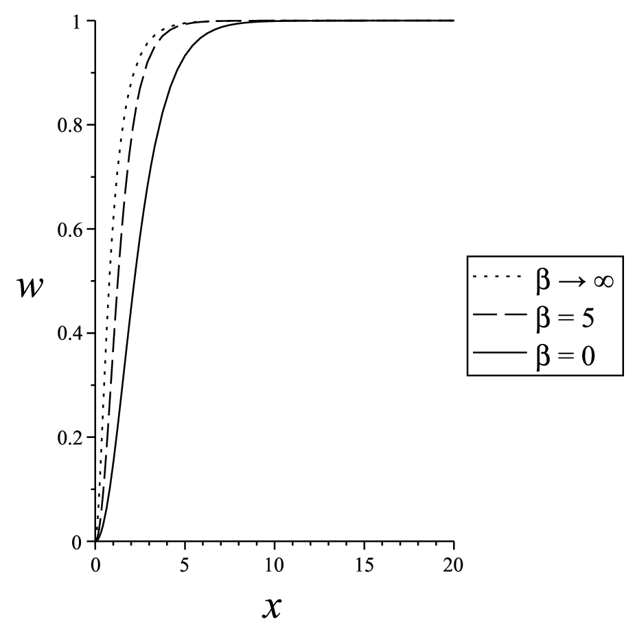
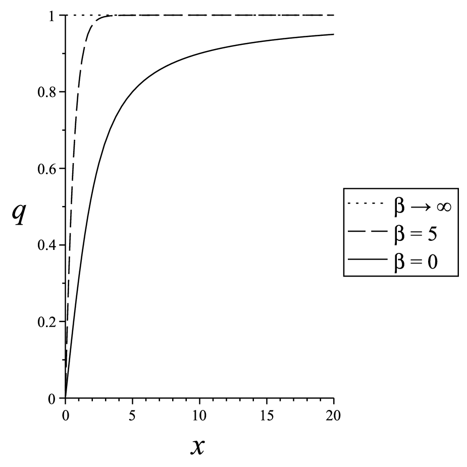
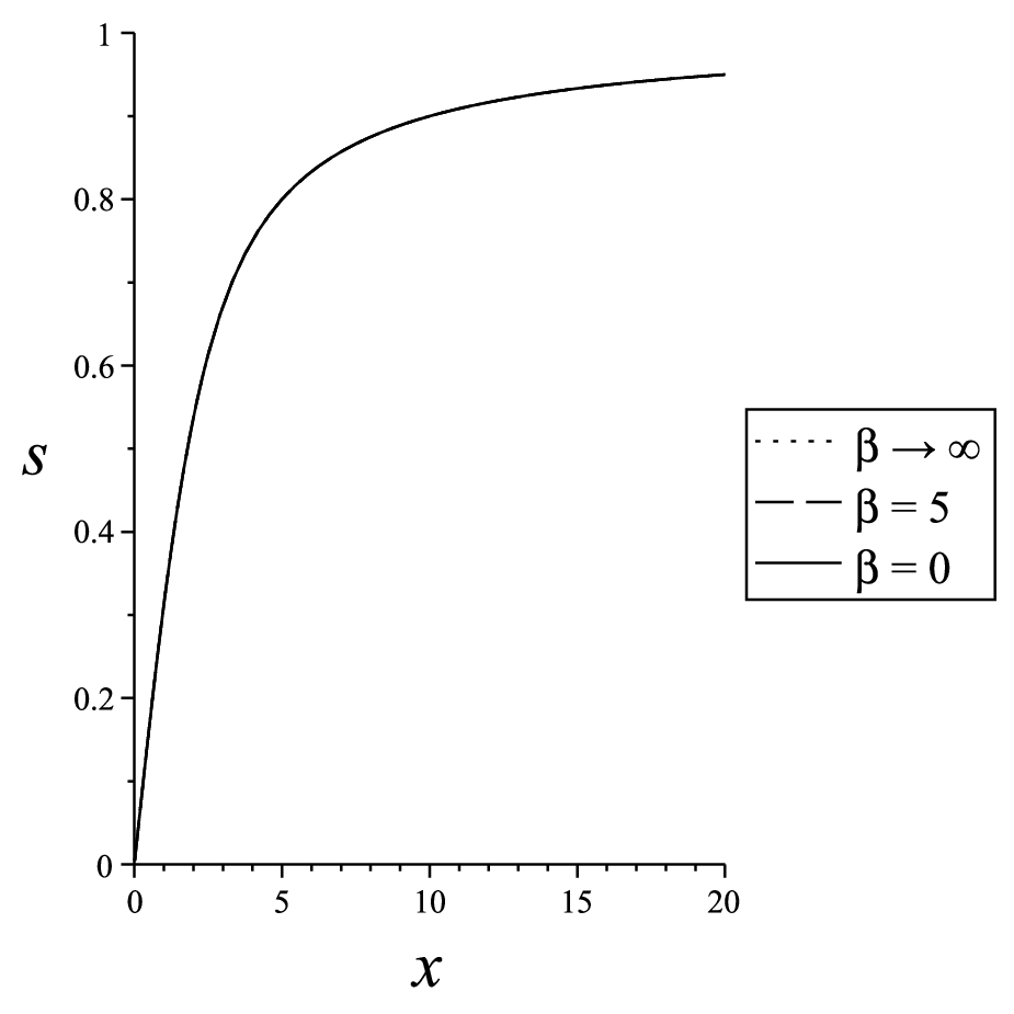
In Figures 1, 2, and 3 we show numerical solutions for $(\frac{g_{e}}{g})^{2}\approx(\frac{g_{m}}{g})^{2}\approx\frac{1}{2}$ when $\beta=5$ and $\beta\rightarrow\infty$. For comparison we also show the solution $\beta=0$, i.e. $\lambda=0$. These two numerical solutions can be used for estimating the quantity $\delta^{2}_{m}$ on whose value the the mass of the dyon depends. Of relevance in performing these calculations and not apparent from Figure 2 is that as $\beta\rightarrow\infty$, $q\approx\sqrt{\beta}x$ for $x<<1/\sqrt{\beta}$. Consequently, we can integrate Equation 3.39, numerically, to obtain

$$\delta^{2}_{m}\approx\begin{cases}.41&\text{for}\;\beta=5,\\ .63&\text{as}\;\beta\rightarrow\infty\>.\end{cases}$$

(3.45)

These results suggest that the mass of the dyon is relatively insensitive to the value of $\beta$, a result alluded to in the work of ’t Hooft.[3]

References

- [1] Howard Georgi. Lie Algebras in Particle Physics. The Benjamin/Cummings Publishing Company, Inc., Reading, Massachussetts, 1982.
- [2] Jeffrey A. Harvey. Magnetic monopoles, duality, and supersymmetry. hep–th/9603086.
- [3] G.’t Hooft. Magnetic monopoles in unified gauge theories. Nuclear Physics, B(79):276–284, 1974.
- [4] C. Montonen and D. Olive. Magnetic monopoles in unified gauge theories. Phys. Lett., 72B:117, 1977.
- [5] Lewis H. Ryder. Quantum Field Theory.–2nd ed., pages 406–414. Cambridge University Press, New York, New York, 1996.
- [6] Heinrich Saller. The central correlations of hypercharge, isospin, colour and chirality in the standard model. hep–th/9802112v1.