The non-singlet kaon fragmentation function from kaon production
Abstract
We perform fits to the available charged and neutral kaon production data in , , and determine the non-singlet combination of kaon fragmentation functions in a model independent way and without any correlations to the other fragmentation functions. Only nuclear isospin invariance is assumed. Working with non-singlets allows us to include the data at very low momentum fractions, which have so far been excluded in global fits, and to perform a first NNLO fit to fragmentation functions. We find that the kaon non-singlet fragmentation function at large is larger than that obtained by the other collaborations from global fit analysis and differs significantly at low .
pacs
12.38.Cy,12.39.St,13.66.Bc,13.87.FhI Introduction
Now that the new generation of high energy experiments with the detection of a final state hadron are taking place, further tests of QCD and the Standard Model require an accurate knowledge not only of the parton distribution functions (PDFs) and , but equally of the fragmentation functions (FFs) . These quantities describe the transition of a parton at factorization scale into a hadron carrying away a fraction of the parton’s momentum or energy in the center-of-mass (c.m.) frame. Like , PDFs and FFs are important quantities because they are universal: according to the factorization theorem, once they are known at some suitably defined scale , they can be calculated at any other scale and used in any type of process. The most reliable way to determine them at a given scale is by fitting to inclusive single hadron production data in which the fraction of available momentum or energy in the c.m. frame carried away by the hadron is measured.
While there has recently been quite an extensive study on the PDFs, only recently have the FFs received more detailed studies, and it has been recognized that alot of uncertainties appear in their determination.
The most direct way to determine the FFs is the one-particle inclusive annihilation process:
| (1) |
Here and from now on we use the shorthand to mean either a or is observed (but not both) in a given event. However, these processes, being proportional to the square of the effective electroweak coupling of the quark , determine only the combinations , i.e. they cannot distinguish the quark and anti-quark FFs. In addition, in the limit of massless quarks, they cannot distinguish between the down-type quark FFs and , which have the same electroweak couplings. Different assumptions are imposed in order to gain more information about the FFs. In order to achieve separate determination of and , the semi-inclusive DIS and the one-hadron inclusive production processes and play an essential role. However, in these processes the nucleon structure is involved, which introduces further uncertainties.
At present several sets of FFs are available in the literature [1], such as Kretzer [2], Kniehl-Kramer-Potter (KKP) [3], Hirai-Kumano-Nagai-Sudoh (HKNS) [4], de Florian-Sassot-Stratmann (DSS) [5], Albino-Kniehl-Kramer (AKK,AKK08) [6, 7], etc. Two points should be noted about them: 1) in the DSS and HKNS analyses, different relations, based on theoretical prejudice, between different initial FFs have been imposed, and 2) there is significant disagreement between the various parametrizations for some of the FFs. It is not clear how much of this disagreement can be attributed to the choices of experimental data used by these collaborations and how much to the choice of the assumptions imposed on the initial FFs. In this paper we shall consider the possibility of obtaining information about the FFs directly from experiment, without any assumptions.
Recently, in [8], we suggested a model independent approach to FFs. We showed that using only C-invariance of strong interactions, the difference cross sections between particle and anti-particle production are expressed solely in terms of non-singlet (NS) combinations of the FFs to any order in perturbative QCD.
There are a number of benefits when performing fits of NS quantities:
i) There are no statistical correlations with gluon FFs, which introduce the largest uncertainties.
ii) In their evolution they do not mix with other FFs, so the difference cross sections are independent of the other FFs at all scales.
iii) The NS components do not contain unresummed soft gluon logarithms (SGLs) at small -values. This allows the use of measurements at much lower values of than in global fit analyses [6, 4, 5, 7], which would (hopefully) better constrain the NS. This would provide stronger tests relative to global fits on the validity of the leading twist calculations at small , where the effects of higher twists, as well as of quark and hadron masses, should be most pronounced.
iv) A next-next-to leading order (NNLO) fit of the non-singlet components is possible, because the perturbative components in the NS sector, namely the splitting and coefficient functions, are known to NNLO. This is in contrast to global fit analyses where only next-to leading order (NLO) calculations of cross sections are possible at present.
Note that here and further on we use the notation for the measured fraction of the energy of the process carried away by the observed hadron , while we use for the fraction of the (unobservable) energy of the fragmenting parton carried by the observed hadron:
| (2) |
i.e. is the measured quantity, is the theoretically QCD-defined quantity, is the c.m. energy of the observed hadron. In leading order (LO), neglecting transverse momenta and hadron mass corrections, and coincide.
In [8] a model independent approach for determining NS combinations of FFs was developed. It was shown that if both charged and neutral kaons are measured in , in or in , SU(2) isospin invariance of strong interactions implies that the cross section differences between the charged and neutral kaons:
| (3) |
always determines, without any assumptions about PDFs and FFs, the non-singlet .
In this paper we apply the model independent approach of [8] to the available data on and production in annihilation and determine the kaon non singlet . This allows us for the first time i) to extract without any assumptions about the unfavoured FFs, commonly used in global fit analysis, ii) to extract without any correlations to other FFs, and especially to , iii) to determine in a larger region than in global fits by using all available data, that is typically in the region , and iii) to perform a first NNLO extraction of the FFs. Including the small data should also improve the precision of the FFs at large since, via the convolution in eq. (4) below, all values in the range contribute, iv) to perform a first phenomenological test of recent NNLO calculations and v) to test, at lower values than before, the incorporation of hadron mass according the procedure of Ref. [9], which becomes more important as decreases.
The rest of the paper is organized as follows. In section II we describe our approach to charged and neutral kaon production. We show how SU(2) invariance allows to single out the NS combination of the kaon FFs, and our basic formula for -kaon production is presented. In section III we describe our method of analysis and justify the choice of the parametrizations used. The results of our fits and the comparison with those obtained from global fits are discussed in section IV. The results are summarized in section V. Appendix A outlines our approach for calculating the Mellin transform of harmonic polylogarithms, which is necessary for the NNLO calculations.
II Our formalism
In this section we describe our approach for extracting the kaon non singlet and contrast it to that in global fits.
In general, the factorization theorem implies that any inclusive hadron production cross section can be written as
| (4) |
where is the energy scale of the process, is the process dependent partonic level cross section for the inclusive production of a parton , determined fully in terms of perturbatively calculable coefficient functions, electroweak factors, and of the PDFs for any initial state hadrons, is the factorization scale, and . Note that though formally is independent of the renormalization scale that appears as the argument of the running coupling , it depends on it when calculated in perturbation theory, further we assume as usually done. In LO the measurable quantity and the QCD variable usually coincide because .
Although the dependence of the fragmentation functions is not calculated perturbatively, QCD determines perturbatively, via the DGLAP evolution equations, their -dependence:
| (5) |
where are the perturbatively calculable splitting functions. In addition, the DGLAP equations allow a choice of which prevents the large logarithms from spoiling the accuracy of the perturbative calculations of . Flavour and charge conjugation symmetry of QCD allow to combine the quark FFs and quark coefficient functions into singlets and non singlets, whose advantage is that they do not mix in their evolution. In this paper we shall deal with non-singlets.
In any kaon-production process, if in addition to the charged -kaons also the neutral -kaons are measured, no new FFs above those used for are introduced in the cross section. This is a consequence of SU(2) invariance of the strong interactions, which relates neutral and charged kaon FFs:
| (6) |
Then for the difference cross section , eq. (3), we obtain the simple expression:
| (7) |
i.e. in any inclusive hadron production process always depends only on one NS combination of FFs, namely . This result relies only on SU(2) invariance for the kaons, eq. (6), and does not involve any other assumptions about PDFs or FFs. It holds in any order in QCD. The explicit expressions for in , SIDIS and scattering were given in Ref. [8].
In this paper, we focus on the most precisely measured and most accurately calculated processes
| (8) |
for which eq.(7) reads:
| (9) |
where is the c.m.energy of the process, , is the Born level cross section for the process , is the number of colours, and is the square of the effective electroweak charge of the quark :
| (10) |
with , the charge of the quark in units of the proton charge, and
| (11) |
We set , , and 4 to estimate the theoretical error, i.e. we consider three different choices for : and . The energy fraction is given by , is the flavour independent perturbatively calculated quark coefficient function:
| (12) |
Eq. (9) is our basic formula which we shall use in our fit to determine .
In our analysis we shall use all available and production data presented by the different collaborations TASSO [10]—[11], MARK II [12], TPC [13], HRS [14], CELLO [15], TOPAZ [16], ALEPH [17], DELPHI [18], OPAL [19]—[20] and SLD [21] at different values of .
Experimental data for hadron production (8) are commonly presented as normalized to the total hadron cross section . From eq.(9) it is clear that the sensitivity of to is determined by the -dependence of . In Fig. 1 the quantities and are shown as functions of , which demonstrates that the biggest contribution would come from data away from the intersections with the -axis and the region between them, namely away from GeV, i.e. most important for our studies would be data for which GeV. It is unfortunate that at the -pole GeV, where the most precise and abundant data exist, the kaon cross section difference normalized to is an extremely small quantity: .

For a large part of the reaction data for kaon production, the primary quark (i.e. the quark at the electroweak vertex) is “tagged”. Experimentally, various techniques are used to achieve this and we refer the reader to the various experimental papers (but see in particular Refs. [45] and [20]). For our calculations, we simply neglect the contributions from all processes except those for which the primary quark is tagged. Since this can be achieved by setting the electroweak charges of all quarks to zero except the tagged quark, the resulting cross section is scheme and scale independent as a physical quantity should be.
III Method of analysis of and data simultaneously
Our formalism would be easy if we had data on and production at identical values of and , with the cross sections being normalized in the same way. Then the optimum procedure to constrain the kaon non singlet would be to fit it to the difference between these data. However, apart from the and quark tagging probabilities from OPAL, this does not hold for the data in general. Data on and are at similar c.m. energies , but usually at quite different values. Therefore we proceed in 4 steps:
1) We combine the measurements on into seven energy intervals 12 – 14.8, 21.5 – 22, 29 – 35, 42.6 – 44, 58, 91.2 and 183 – 186 GeV and parametrize the dependence of the cross section for -production in each interval separately as defined below in eq. (19).
2) For each interval of we calculate perturbatively, using eq. (9), parametrizing the dependence of the kaon non singlet at a suitable starting scale , as described below in eq. (20).
3) Using (19) and (20) we calculate the charged kaon cross section in each energy interval of through the expression:
| (18) |
4) We fit the parameters in (as given in eq. (19)) and the parameters in the kaon non singlet (as given in eq. (20)) simultaneously to measurements of charged and neutral kaon production in reactions.
We believe that the above approach is the optimum one since it involves performing only one fit.
Since the perturbative calculation of the cross section difference is free of SGLs, it is expected to be valid at much lower values of than the perturbative calculations of and separately. Therefore in our fits we vary the lowest value of that the data can take. In global fit analyses the usual minimum bound of – was used, but in general we will include data at lower values.
We parametrize the cross section as follows:
| (19) |
where , , , , , and are seven different parameters that are fitted to the data in each range of separately. The term is motivated by the dependence of the cross section on predicted by QCD. In the case where data of only one value exists, namely the data at 58 and 91.2 GeV, is fixed to zero. Otherwise, note that no QCD input is used for the calculation of the production data. The motivation behind the choice of the parametrization is empirical, although the behaviour at large and the at small also follow from resummation in perturbative QCD in these respective regions for .
Due to flavour symmetry, vanishes whenever the quark at the electroweak vertex is neither a nor -quark. Thus, we do not need the , and -quark tagged data from OPAL that should automatically cancel and cannot constrain the kaon non singlet in our approach. However, we shall use the light-quark tagged data, that contain the and -quarks. We can parametrize these data directly, but instead we parametrize and quark tagged data as in eq. (19), and calculate the light quark tagged cross section as the difference between the untagged cross section and the sum of the and quark tagged cross sections. By including all available heavy quark tagged data in this way, we hope to improve our calculation of the light quark tagged data. Thus we have 9 parametrized functions in to describe all the data: seven parametrizations for the untagged data in each -energy interval and 2 for the and quark tagged cross sections at GeV.
For the calculation of using eq. (9), we require a parametrization for the kaon non singlet at a starting scale which satisfies the following conditions: It should exhibit the power-like behaviour as . Note that the resummed double logarithmic contribution to the splitting functions suggests that a Gaussian behaviour in at small occurs only for the gluon and singlet FFs [24] and we do not assume that this behaviour occurs also for the non singlet. The FF should also exhibit the behaviour as z approaches 1. After trying various parametrization that were in accordance with the above requirements, we found that the best parametrization, i.e. the one that gave a good fit with all parameters well constrained by the data (meaning that the parameters did not become large), was
| (20) |
This parametrization is effectively the same as the one used in the latest global fits in [5, 7], except that in order to allow a larger function space at small to be available to the non singlet.
To be clear, our main fit (discussed in subsection IV.2) which determines the NS proceeds as follows. We determine in a simultaneous fit to and production data – we fit the production data to eq. (19) and we fit the production data to the difference of eq. (19) (multiplied by 2) and : , where is calculated from using eq. (7). Note that if all the production data were measured at the same and values, and defined in the same way, as the production data, there would be no need for eq. (19) — we would simply fit the theoretical calculation of , eq. (7), directly to the measurements of at each measured and value. We stress that, despite the theoretical discussion immediately following eq. (19), the motivation for the parameterization in eq. (19) is mainly empirical – as we will see in subsection IV.1, such a parameterization describes all production data well. We note, however, that different parameterizations will exist which give an equally good fit to the production data but give slightly different results. Such a “parameterization error” should in any case be less than the errors on the parameters due to the errors on the measurements. We also note that a single simultaneous fit of all parameters to all data is the statistically correct approach. For example, fitting the parameters in eq. (19) to the production data and then, as a separate fit, fitting the parameters in eq. (20) to the data only would not take into account the fact that the fitted values of the the parameters in eq. (19) carry significant experimental errors.
In our perturbative calculations, we choose GeV, 5 active flavours , and MeV. We perform all calculations in Mellin space since this approach is numerically more efficient than explicitly performing space convolutions such as that in eq. (20).
The NNLO perturbative components for the cross section difference can be obtained using the results of [25] for the non singlet coefficient functions and the results of [26] for the difference between the spacelike and timelike non singlet splitting functions. The former, as well as the spacelike non singlet splitting functions of [27], are presented in Mellin space as a weighted sum of harmonic sums. The latter is presented in space as a weighted sum of harmonic polylogarithms. Our approach for determining the Mellin transform of these harmonic polylogarithms is discussed in Appendix A.
Because the effect of the observed hadron’s mass is expected to be significant at low , we incorporate the hadron mass effects according to the method of Ref. [9]. In this case, the scaling variable , which in the factorization theorem is defined as the ratio of the detected hadron’s light cone momentum to the overall process’s, must be distinguished from the energy and momentum fractions measured in experiment and given by
| (21) |
respectively. We stress that and equal only when hadron mass effects are neglected. Otherwise, they are related to via:
| (22) |
The cross sections and that determine , eq. (9), which we are calculating and which enters the factorization theorem, are related to the measurable ones and via [9]:
| (23) | |||||
| (24) |
where stands for either or . We exploit the fact that different data groups use different definitions for “” in order to obtain the kaon mass, by using the above relations and fitting the mass . We assume the masses of the neutral and charged kaons are equal. We note that fitting
The total number of free parameters in our fits to charged and neutral kaon data is 66, and the total number of data points is 730.
We could choose to fit the data at a subset of values and then predict the remaining data using the universality of the non singlet FF thus obtained. However, we choose to simultaneously fit all the available data in order to maximize the constraints on the parameters appearing in eq. (20). As we will see in section IV, the simultaneous description of all data with the same fitted non singlet FF turns out to be good, in accordance with the universality of FFs.
IV Results of the analysis
First we perform a fit only to the available production data in order to ensure that the parametrization in eq. (19) is adequate for the data that we will use in our extractions of the kaon non singlet. Then we perform a simultaneous fit to both charged and neutral kaon production data in reactions. In the latter case we perform our analysis to NLO and NNLO in perturbative QCD.
IV.1 Analysis of data
Here we present our results from a fit to data only, using the parametrizations in eq. (19). The average per data point, , for each data set is presented in Table 1 together with details of the data set. Also shown, where applicable, is the value at the global minimum of for each data set, which after multiplication by the normalization error is the most likely systematic deviation of the central values (see Ref. [7] for a complete discussion), and which should obey for a reasonable fit.
| Collaboration | Cross section | Tagging | # | Norm. | |||
| (GeV) | data | (%) | |||||
| TASSO [10] | untagged | 14.0 | 9 | 15 | 0.4 | -0.6 | |
| TASSO [28] | untagged | 14.8 | 9 | 0.3 | -0.4 | ||
| TASSO [28] | untagged | 21.5 | 6 | 0.0 | |||
| TASSO [10] | untagged | 22.0 | 6 | 0.1 | 0.1 | ||
| HRS [14] | untagged | 29 | 13 | 3.2 | |||
| MARK II | untagged | 29.0 | 21 | 12 | 0.8 | 0.3 | |
| TPC [13] | untagged | 29 | 8 | 0.5 | |||
| TASSO [29] | untagged | 33.3 | 9 | 15 | 0.7 | 0.2 | |
| TASSO [10] | untagged | 34.0 | 15 | 1.4 | -0.1 | ||
| TASSO [28] | untagged | 34.5 | 15 | 1.3 | |||
| CELLO [15] | untagged | 35 | 11 | 0.5 | |||
| TASSO [28] | untagged | 35 | 15 | 1.3 | |||
| TASSO [28] | untagged | 42.6 | 15 | 0.5 | |||
| TOPAZ [16] | untagged | 58 | 7 | 0.1 | |||
| ALEPH [30] | untagged | 91.2 | 30 | 2 | 0.5 | -2.3 | |
| DELPHI [31] | untagged | 91.2 | 26 | 0.7 | |||
| OPAL [19] | untagged | 91.2 | 20 | 6 | 1.0 | -1.1 | |
| OPAL [20] | c tagged | 91.2 | 5 | 0.6 | |||
| OPAL [20] | b tagged | 91.2 | 5 | 1.7 | |||
| SLD [32] | untagged | 91.2 | 17 | 1.1 | |||
| SLD [32] | l tagged | 91.2 | 17 | 0.6 | |||
| SLD [32] | c tagged | 91.2 | 17 | 0.7 | |||
| SLD [32] | b tagged | 91.2 | 17 | 1.5 | |||
| DELPHI [33] | untagged | 189 | 10 | 0.7 | |||
| DELPHI [33] | untagged | 183 | 8 | 1.3 | |||
| 331 | 1.1 |
In general, as seen from the Table, our parametrization provides a good description of all but the HRS data, where the description is poor. At GeV, the quark tagged data appears to be slightly inconsistent with the other data. The value of for the ALEPH data is high, but the fit to the other data at GeV in general is good. Otherwise, both and which suggests that the parametrization in eq. (19) is sufficient to represent these data.
In the caption of Table 1 we quote the fitted kaon mass MeV, which is somewhat smaller than the true mass of 498 MeV. However, it is not significantly different from the value 343 MeV obtained in global fit analyses in Ref. [7], where it was argued that kaon production through complex decay chains may cause a significant difference between the true mass and the fitted mass, when only direct parton fragmentation is assumed in the calculations.
IV.2 Analysis of and
Here we present the results from the combined analysis of and data.
We implement large resummation in our NLO analysis. We resum both leading and next-to-leading logarithms (LL and NLL respectively), which are all the classes of logarithms appearing at this order. As shown in the AKK08 fit [7], this significantly improves fits to charged kaon data at large . Resummation in the quark cross section (or quark coefficient function) is obtained from the method of Ref. [34] and the results for the unfactorized partonic cross section in Ref. [35], while resummation in the evolution is performed according to the method in Ref. [36].
Thus we apply the two most optimum theoretical tools to our calculations, namely the NLO results with resummation, and the NNLO without resummation.
The measured inclusive and production cross sections and the obtained values, both in NLO and NNLO, are shown in Table 2.
| Collaboration | Cross section | Tagging | # | Norm. | |||||
| (GeV) | data | (%) | NLO | NNLO | |||||
| TASSO [37] | untagged | 12 | 3 | 20 | 1.0 | -1.1 | 0.9 | -1.0 | |
| TASSO [38] | untagged | 14 | 9 | 8.5 | 1.0 | -0.1 | 0.9 | -0.2 | |
| TASSO [38] | untagged | 22 | 10 | 6.3 | 0.3 | -0.5 | 0.3 | -0.6 | |
| HRS [14] | untagged | 29 | 7 | 1.9 | 2.3 | ||||
| MARKII [12] | untagged | 29 | 6 | 12 | 2.1 | -1.4 | 2.6 | -1.4 | |
| TPC [39] | untagged | 29 | 29 | 1.2 | 1.8 | ||||
| TASSO [37] | untagged | 30 | 5 | 20 | 0.9 | -1.4 | 0.9 | -1.4 | |
| TASSO [11] | untagged | 34 | 11 | 6 | 1.5 | -1.0 | 1.6 | -0.9 | |
| TASSO [11] | untagged | 44 | 4 | 6 | 0.1 | 0.1 | |||
| TOPAZ [16] | untagged | 58 | 12 | 0.7 | 0.7 | ||||
| ALEPH [17, 30] | untagged | 91.2 | 29 | 3 | 1.3 | -0.6 | 1.2 | -0.7 | |
| DELPHI [18] | untagged | 91.2 | 23 | 0.2 | 0.2 | ||||
| DELPHI [18] | l tagged | 91.2 | 23 | 0.8 | 0.8 | ||||
| DELPHI [18] | b tagged | 91.2 | 23 | 0.5 | 0.5 | ||||
| OPAL [40] | untagged | 91.2 | 33 | 2.3 | 2.5 | ||||
| OPAL [20] | c tagged | 91.2 | 5 | 4.6 | 4.8 | ||||
| OPAL [20] | b tagged | 91.2 | 5 | 4.5 | 4.4 | ||||
| SLD [21] | untagged | 91.2 | 36 | 1.9 | 1.5 | ||||
| SLD [21] | l tagged | 91.2 | 36 | 4.7 | 4.0 | ||||
| SLD [21] | c tagged | 91.2 | 36 | 2.7 | 2.4 | ||||
| SLD [21] | b tagged | 91.2 | 36 | 4.7 | 4.6 | ||||
| DELPHI [33] | untagged | 189 | 8 | 5.2 | 5.3 | ||||
| OPAL [20] | u tagged | 91.2 | 5 | 1.2 | 1.4 | ||||
| OPAL [20] | d tagged | 91.2 | 5 | 1.0 | 1.5 | ||||
| TASSO [10] | untagged | 14 | 9 | 15 | 0.4 | -0.2 | 0.4 | 0.0 | |
| TASSO [28] | untagged | 14.8 | 9 | 0.6 | 0.6 | ||||
| TASSO [28] | untagged | 21.5 | 6 | 0.1 | 0.1 | ||||
| TASSO [10] | untagged | 22 | 6 | 0.2 | 0.2 | 0.3 | 0.3 | ||
| HRS [14] | untagged | 29 | 13 | 2.9 | 3.4 | ||||
| MARK II | untagged | 29 | 21 | 12 | 1.2 | 1.2 | 1.3 | 1.4 | |
| TPC [13] | untagged | 29 | 8 | 1.8 | 2.3 | ||||
| TASSO [29] | untagged | 33.3 | 9 | 15 | 0.6 | 0.3 | 0.7 | 0.4 | |
| TASSO [10] | untagged | 34 | 15 | 1.3 | 0.0 | 1.3 | 0.0 | ||
| TASSO [28] | untagged | 34.5 | 15 | 1.3 | 1.2 | ||||
| CELLO [15] | untagged | 35 | 11 | 0.6 | 0.6 | ||||
| TASSO [28] | untagged | 35 | 15 | 1.9 | 1.9 | ||||
| TASSO [28] | untagged | 42.6 | 15 | 0.6 | 0.6 | ||||
| TOPAZ [16] | untagged | 58 | 7 | 1.1 | 1.0 | ||||
| ALEPH [30] | untagged | 91.2 | 30 | 2 | 1.5 | 1.9 | 1.4 | 1.7 | |
| DELPHI [31] | untagged | 91.2 | 26 | 3.0 | 2.8 | ||||
| OPAL [19] | untagged | 91.2 | 20 | 6 | 2.3 | 0.4 | 2.2 | 0.3 | |
| OPAL [20] | c tagged | 91.2 | 5 | 1.2 | 1.3 | ||||
| OPAL [20] | b tagged | 91.2 | 5 | 12.9 | 12.8 | ||||
| SLD [32] | untagged | 91.2 | 17 | 3.2 | 3.0 | ||||
| SLD [32] | l tagged | 91.2 | 17 | 0.8 | 0.7 | ||||
| SLD [32] | c tagged | 91.2 | 17 | 1.2 | 1.2 | ||||
| SLD [32] | b tagged | 91.2 | 17 | 5.1 | 5.2 | ||||
| DELPHI [33] | untagged | 183 | 8 | 1.9 | 1.9 | ||||
| DELPHI [33] | untagged | 189 | 10 | 2.7 | 2.7 | ||||
| 730 | 2.3 | 2.2 |
In general, with the exception of a few data sets, in particular the quark tagged cross section measurements, the description of the data is rather good. However, the kaon mass, both in NLO and NNLO, is significantly lower than the one obtained in the phenomenological description of the data (see Table 1) only, i.e. without perturbative QCD, also it is significantly lower than the value 343 MeV obtained in Ref. [7].


Our results for in NLO are shown in Fig. 2. In the same figure the NLO results from global fits of the DSS, HKNS and AKK08 sets are presented as well. As seen from the figure, at there is an agreement in shape among the different plots of the NS, but our NS is in general larger in magnitude. However, they differ significantly at . The most striking difference is the negative value for the NS at obtained in our approach, while all global fit parametrizations imply a positive .
In Tables 3 — 5 we show the values of the parameters for our main fit, NLO + resummation. However, we caution the reader that, because we begin our evolution at GeV, due to neglect of higher order NNLO terms, the uncertainties on these parameters in the NLO calculation may be very large and thus may depend significantly on the method used for solving the DGLAP equations. This uncertainty is approximately equal to the size of the NNLO terms.
| Parameter | Value |
|---|---|
| -6.25 | |
| -0.11 | |
| 3.12 | |
| 11.13 | |
| 0.60 | |
| 3.01 |
| energy interval in [GeV] | N | A | B | c | d | e | |
|---|---|---|---|---|---|---|---|
| 12 14.8 | -17.2 | -2.33 | 10.1 | -2.99 | -0.357 | ||
| 21.5 22 | 14.5 | 12.2 | -7.24 | 1.45 | |||
| 29 35 | -0.444 | 3.81 | -2.57 | 3.49 | 1.79 | -0.696 | |
| 42.6 44 | 4.91 | 7.10 | -1.66 | ||||
| = 58 | 6.03 | 0 (fixed) | -1.23 | 6.26 | 1.11 | -0.415 | |
| = 91.2 | 0 (fixed) | -4.88 | -0.681 | 1.68 | -0.338 | ||
| 183 189 | -646. | -1.34 | 5.16 | 0.492 | -0.156 |
| the data | N | A | B | c | d | e | |
|---|---|---|---|---|---|---|---|
| tagged | 2.62 | 0 (fixed) | -7.52 | 2.39 | 3.97 | -1.01 | |
| -tagged | 0.164 | 0 (fixed) | -8.65 | 2.01 | 2.95 | -0.474 |
In order to understand the origin of the negative value of obtained from the difference cross sections , we make a comparison of the charged and neutral kaon production data at various in Fig. 3.


Such a direct comparison is possible because, for these data, the cross section measurements happen to be defined the same way, i.e. they are differential in the same variable and normalized in the same way, which is not typical for the data in general. In general, the description of these data is good. According to the (data-theory)/theory plots, the calculation for the production data tends to overshoot the central values of the data, while for production the behaviour is the opposite, but this is not significant relative to the experimental errors. For , the calculated charged kaon production exceeds the neutral except when GeV. However, below this region in the opposite behaviour is observed, i.e. for , for all except GeV, where and are very similar. As Fig. 1 shows, the sign of the difference of the effective electroweak couplings of the and quark flavours, for all except around the -pole ( GeV2), is positive, i.e. for GeV2 and GeV2, i.e. at the cross sections that give the main contribution to the NS in (9). Then, following the simple LO approach in which convolutions are replaced by ordinary products, eq.(9) implies that at , and at . Of course these rough arguments do not take into account experimental errors, which are rather big for kaon production, or convolutions etc., however they do help to verify the result qualitatively.
Our negative result for at low , though justified by the above arguments on the data on , is however in contrast to the intuitive interpretation for favoured -quark and unfavoured -quark transitions. In addition, our result is quite different from the DSS, AKK08 and HKNS results. There could be several reasons for this, as well as for the unexpectedly low values for the kaon mass MeV and MeV, shown in Table 2. Most probably it is due to the different assumptions in the parametrizations and to inclusion of the small -data in our fit. The DSS and HNKS collaborations use the assumption that all light quark unfavoured FFs are equal: , while no assumptions were used in the AKK08 fit and in the analysis in this paper, denoted by AC. The fact that the DSS and HKNS non singlet FF, which can be written as , is lower than the others for in Fig. 2 suggests that and may be overestimated in this region when the light quark unfavoured FFs are fixed to be equal to one another. Maybe this could explain the similarity of the results for obtained from the DSS and HKNS fits on one hand, and of AKK08 and AC at on the other hand (see Fig. 2). The AKK08 and HKNS analyses used no data below , the DSS analysis used only data at , while we include data as low as . The discrepancy may also be a result of various low effects not accounted for in the calculation, such as dynamical higher twist, quark mass corrections, etc. However, perhaps the most likely reason are the large experimental errors on the NS. The FFs of the various collaborations should be the same within the error (composed of the theoretical errors and the (unknown) experimental errors propagated from the fitted data to the FF). Thus if we assume that the various FFs are consistent, then the spread of FFs in Fig. 2 gives some indication of the error on the FF, and shows the error increasing drastically with decreasing . This argument assumes that the (similar) assumptions made on the FFs in the DSS and HKNS fits are correct. In any case, these results warrant further investigation into the validity of the standard approach at low . It is promising, however, that it is possible to fit low data () using fixed order perturbation theory.
The negative value of the non singlet FF at low contradicts the physical argument that favoured FFs are larger than unfavoured FFs. This behaviour alone is not too serious since FFs in general are not physical. However, the second Mellin moment of a FF is physical, in the sense of being factorization scheme and scale independent, and can be interpreted as the fraction of momentum of the fragmenting parton that is carried away by hadrons of species . The second moment of the non singlet FF is expected then to be positive, but from our fit using calculations to NLO (NNLO) the result is -0.07 (-0.1). Most likely this is a consequence of the large experimental errors at low . However, it could also arise from a breakdown of perturbation theory, or from effects not accounted for in the calculation at low , if such effects turn out significantly large.
In order to check our negative result for the NS at small , we performed a fit in which a parameterization of the form , instead of that in eq. (20), was used which yielded a positive NS (i.e. ). However, the result was obtained, which corresponded to a of about 100 points above that for our main fit. Thus the parametriztion in eq. (20) is much more favoured by the data. We also performed a fit in which the NS was fixed to zero, and obtained again. Thus a positive, as well as a zero kaon non singlets are both allowed by data as a whole, but the fits are much worse. Note that in our analysis we include data at very low , which are the most accurate data and any deviations of the fit from these data immediately results in higher . It is the small data that raises with the zero and parameterizations.


In Fig. 4 we compare the NLO and NNLO fits for at GeV (Fig. 4, left) and at GeV (Fig. 4, right) for various choices of the factorization scale , . As seen from this figure, there is an extremely strong dependence on the choice of and on the chosen perturbative order – NLO or NNLO. The quality of the fits for all curves is good, which indicates that the errors of the available data are too big to constrain the non-singlet FFs. With very accurate data, the spread of the three NLO FFs and the spread of the three NNLO FFs should be less and, assuming that the theoretical error in the calculations is sufficiently larger than the experimental error, both should give some indication of the theoretical error. However, since large x resummation has been applied only to the NLO calculation and not in NNLO, this analysis cannot test the perturbative convergence by comparing NLO and NNLO calculations. Also the low -data, for the first time included in an analysis, might have caused troubles. Fig. 4 implies only upper and lower bounds on the non-singlet: 0 0.2 at .
Note that in the used method, the uncertainties of the FFs are due almost completely to the experimental errors on the data. The theoretical error in the calculation is relatively negligible here. Having the experimental errors as they are, one would not get such good fits to the NS FF from cross section (not cross section difference) measurements, even with similarly large errors. One of the reasons is that, due to the large -logarithms in the singlet / gluon evolution and in gluon coefficient functions, the small -data cannot be included in the analysis. All curves are positive for , and the theoretical error in this region is arguably less for the NNLO fits. More accurate data is needed to better determine the scale variation.
The non singlet FF from the NNLO fit with is close to zero for , suggesting that the cross section is too. This is a consequence of the fact that the production data and the production data (multiplied by 2) are very close (see Fig. 3). This behaviour is consistent with our finding above, that a good fit can be obtained with the non singlet FF fixed to zero (i.e. all parameters in eq. (20) fixed to zero so that only the parameters in eq. (19) are varied in the fit).
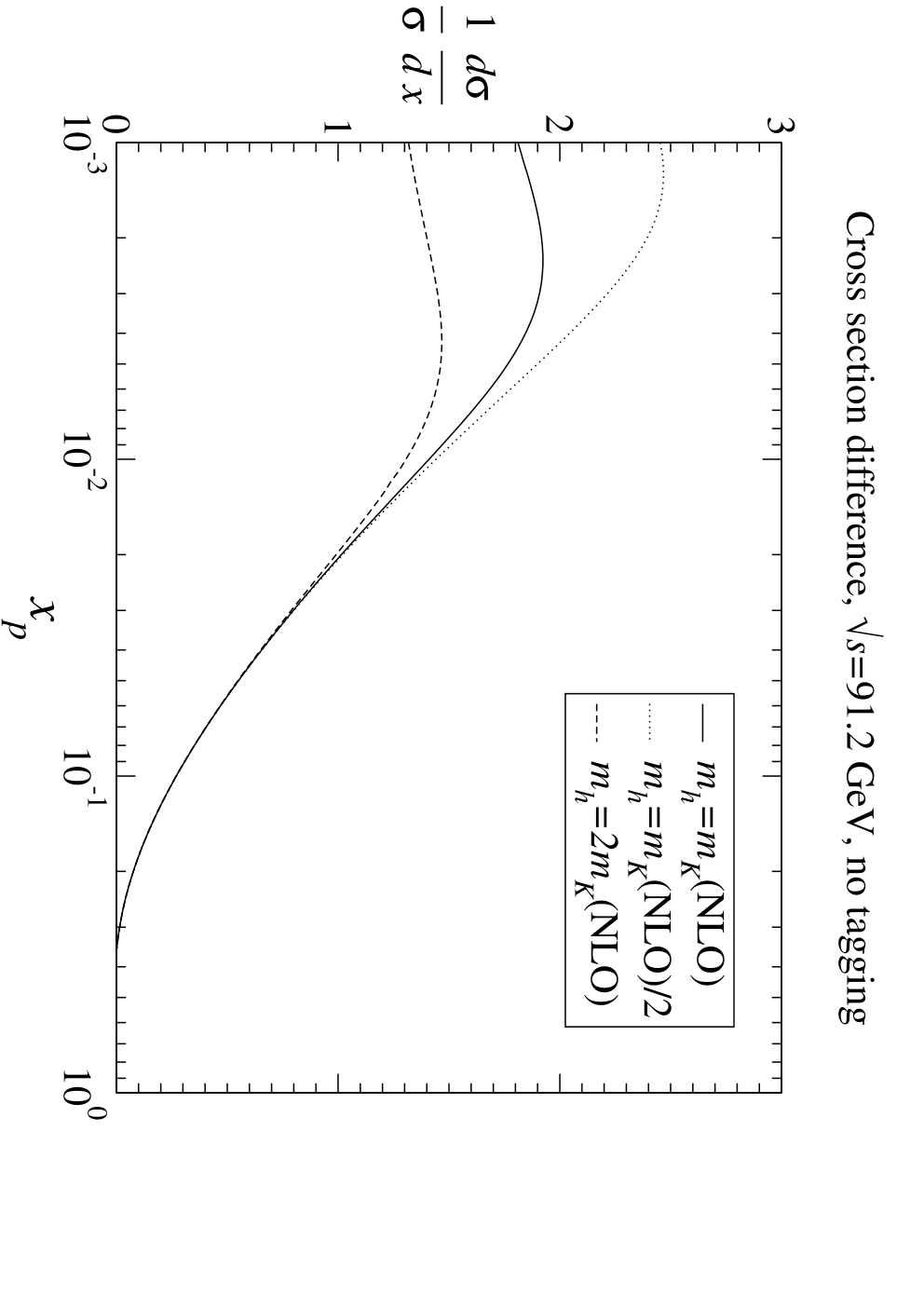
In Fig. 5, we examine the sensitivity of the cross section difference to the mass for two different values of , taking the mass to be , and in eq. (22), where is the fitted mass. As shown in the figure, for = 10 GeV the calculation becomes sensitive to at , while for the sensitivity sets in at where most of the data lie. Because the calculation is very sensitive to hadron mass effects at low and small , these effects strongly affects our fits. Conversely, precisely because the hadron mass effects are important for the data in this region means that they cannot be neglected. However, other low , small effects, such as higher twist and mass effects of resonances from which the kaon has been produced, will also be absorbed into after it has been fitted. More accurate data will be needed to determine how important these other effects are.

In Fig. 6 we show the effect on the fitted NS of increasing the lower bound in on the data. The result when no cut is imposed is similar to the result with a cut of , implying that data for which might not impose important constraints. The largest change in the fitted NS is from to . The fact that this difference is so large suggests that a new (but valid) minimum in has been found. This implies that the accuracy of the data at is not enough to form the difference cross sections with the required precision to determine . In particular, note the unphysical divergence of the FF as , which is caused by the negative values of the fitted and parameters in eq. (20), which further indicates the inability of the data at to constrain the FF at large . Only including the large amount of precise small data, which through convolution determines the not only at , but also at all , allows to determine the NS in the whole region.


V Summary
The cross section difference determines uniquely the NS without any assumptions. We have extracted from kaon production in and compared our results to those from global fit analyses, namely the DSS, the HNKS and the AKK08 parametrizations. In contrast to global fits, in our analysis i) data at much lower values of , as low as , could be included in the fit because of the absence of SGLs in NS perturbative quantities, ii) calculations could also be performed at NNLO and iii) no assumptions about unfavoured FFs were imposed. The quality of the fits were high suggesting that perturbative QCD is consistent with the data, including the very low measurements. However, the fitted kaon mass , on which low cross sections depend strongly, was found to be somewhat lower than the value obtained phenomenologically, i.e. without perturbative QCD, from the fit to neutral kaon production data only. The obtained values for at small are negative and considerably different from those obtained from global analyses. Fits performed using NNLO calculations gave lower theoretical errors on , suggesting stability of the perturbation series for the most of the available cross section measurements.
The current measurements of inclusive kaon production are not at the level of accuracy required to obtain a competitive extraction of from the considered cross section differences. Also it is not enough to really constrain the non-singlet . As our fits show, the error on the FF is large (see Fig. 4). But our method is a good one, which allows for the first NNLO analysis of inclusive hadron production and it will be useful for future studies. Admittedly the experimental errors are large, still one would not get such good fits to cross section (not cross section difference) measurements, even with similarly large errors, due to small -logarithms in singlet / gluon evolution and in gluon coefficient functions.
With more accurate data in the future and in greater number, it would be nice to see if we could continue to describe the low data well. In particular, at present the most accurate data is that for which GeV, which is the least sensitive to the kaon non singlet due to the similarity between the and quark effective electroweak charges at this energy. However, such an extraction may become possible once the accurate measurements of kaon production at BaBar [41] have been finalized, because these data are at GeV where the quark electroweak charges are very different. These BaBar data could also significantly improve the constraints on .
Appendix A Harmonic polylogarithms in Mellin space
In this section we describe our procedure for obtaining the Mellin transform of harmonic sums, defined as
| (25) |
where
| (26) |
Their Mellin transforms can be expressed as a weighted sum of harmonic sums, defined for integer values of the Mellin space variable as
| (27) |
which can be continued to complex according to the procedure in [42].
Such weighted sums can be found recursively [43] by determining, in Mellin space, the dependence of a harmonic polylogarithm on the same one without the leftmost index. By performing the integration for the Mellin transform of by parts, which gives , and then performing the replacements , we find that our desired relations are
| (28) |
| (29) |
| (30) |
where and the “+” distribution can be calculated from by expanding as a series in before performing the Mellin transform. The result [44] is simply that, because which follows from eq. (27), where here and in what follows, each term of the form
| (31) |
becomes
| (32) |
Furthermore, each term of the form
| (33) |
becomes
Although the are singular, they may be treated in a symbolic sense because , and are all finite when the real part of is suitably large. To complete this recursive procedure, we require the Mellin transforms of the simplest harmonic polylogarithms, which are given by
| (35) |
A Mathematica file for implementing this procedure and for producing FORTRAN programs
to calculate numerical values of harmonic polylogarithms anywhere in Mellin space
can be obtained from http://www.desy.de/~simon/HarmonicSums.
Acknowledgements.
The authors would like to thank E. Leader for a careful reading of the early draft of the manuscript and for numerous discussions. The work of E. C. was supported by HEPTools EU network MRTN-CT-2006-035505 and the Bulgarian National Science Foundation, Grant 288/2008.References
- [1] S. Albino, arXiv:0810.4255 [hep-ph], to be published in Reviews of Modern Physics.
- [2] S. Kretzer, Phys. Rev. D 62 (2000) 054001 [arXiv:hep-ph/0003177].
- [3] B. A. Kniehl, G. Kramer and B. Pötter, Nucl. Phys. B 582 (2000) 514 [arXiv:hep-ph/0010289].
- [4] M. Hirai, S. Kumano, T. H. Nagai and K. Sudoh, Phys. Rev. D 75 (2007) 094009 [arXiv:hep-ph/0702250].
- [5] D. de Florian, R. Sassot and M. Stratmann, Phys. Rev. D 76 (2007) 074033 [arXiv:0707.1506 [hep-ph]]; Phys. Rev. D 75 (2007) 114010 [arXiv:hep-ph/0703242].
- [6] S. Albino, B. A. Kniehl and G. Kramer, Nucl. Phys. B 725 (2005) 181 [arXiv:hep-ph/0502188]; Nucl. Phys. B 734 (2006) 50 [arXiv:hep-ph/0510173].
- [7] S. Albino, B. A. Kniehl and G. Kramer, Nucl. Phys. B 803 (2008) 42 [arXiv:0803.2768 [hep-ph]].
- [8] E. Christova and E. Leader, Phys. Rev. D79 (2009) 014019 [arXiv:0809.0191 [hep-ph]]; Eur. Phys. J. C 51 (2007) 825 [arXiv:hep-ph/0612049].
- [9] S. Albino, B. A. Kniehl, G. Kramer and W. Ochs, Phys. Rev. D 73 (2006) 054020 [arXiv:hep-ph/0510319].
- [10] TASSO Collaboration, M. Althoff et al., Z. Phys. C 27 (1985) 27.
- [11] TASSO Collaboration, W. Braunschweig et al., Z. Phys. C 42 (1989) 189.
- [12] MARK II Collaboration, H. Schellman et al., Phys. Rev. D 31 (1985) 3013.
- [13] TPC/Two Gamma Collaboration, H. Aihara et al., Phys. Rev. Lett. 53 (1984) 2378.
- [14] HRS Collaboration, M. Derrick et al., Phys. Rev. D 35 (1987) 2639.
- [15] CELLO Collaboration, H. J. Behrend et al., Z. Phys. C 46 (1990) 397.
- [16] TOPAZ Collaboration, R. Itoh et al., Phys. Lett. B 345 (1995) 335 [arXiv:hep-ex/9412015].
- [17] ALEPH Collaboration, D. Buskulic et al., Z. Phys. C 66 (1995) 355.
- [18] DELPHI Collaboration, P. Abreu et al., Eur. Phys. J. C 5 (1998) 585.
- [19] OPAL Collaboration, G. Abbiendi et al., Eur. Phys. J. C 17 (2000) 373 [arXiv:hep-ex/0007017].
- [20] OPAL Collaboration, G. Abbiendi et al., Eur. Phys. J. C 16 (2000) 407 [arXiv:hep-ex/0001054].
- [21] SLD Collaboration, K. Abe et al., Phys. Rev. D 69 (2004) 072003 [arXiv:hep-ex/0310017].
- [22] S. A. Larin and J. A. M. Vermaseren, Phys. Lett. B 303 (1993) 334 [arXiv:hep-ph/9302208].
- [23] P. M. Nadolsky et al., Phys. Rev. D 78 (2008) 013004 [arXiv:0802.0007 [hep-ph]].
- [24] S. Albino, B. A. Kniehl and G. Kramer, Eur. Phys. J. C 38 (2004) 177 [arXiv:hep-ph/0408112].
- [25] P. J. Rijken and W. L. van Neerven, Phys. Lett. B 386 (1996) 422 [arXiv:hep-ph/9604436]; Nucl. Phys. B 487 (1997) 233 [arXiv:hep-ph/9609377]; J. Blumlein and V. Ravindran, Nucl. Phys. B 749 (2006) 1 [arXiv:hep-ph/0604019]; A. Mitov and S. O. Moch, Nucl. Phys. B 751 (2006) 18 [arXiv:hep-ph/0604160].
- [26] A. Mitov, S. Moch and A. Vogt, Phys. Lett. B 638 (2006) 61 [arXiv:hep-ph/0604053].
- [27] S. Moch, J. A. M. Vermaseren and A. Vogt, Nucl. Phys. B 688 (2004) 101 [arXiv:hep-ph/0403192].
- [28] TASSO Collaboration, W. Braunschweig et al., Z. Phys. C 47 (1990) 167.
- [29] TASSO Collaboration, R. Brandelik et al., Phys. Lett. B 105 (1981) 75.
- [30] ALEPH Collaboration, R. Barate et al., Phys. Rept. 294 (1998) 1.
- [31] DELPHI Collaboration, P. Abreu et al., Z. Phys. C 65 (1995) 587.
- [32] SLD Collaboration, K. Abe et al., Phys. Rev. D 59 (1999) 052001 [arXiv:hep-ex/9805029].
- [33] DELPHI Collaboration, P. Abreu et al., Eur. Phys. J. C 18 (2000) 203 [Erratum-ibid. C 25 (2002) 493] [arXiv:hep-ex/0103031].
- [34] S. Albino and R. D. Ball, Phys. Lett. B 513 (2001) 93 [arXiv:hep-ph/0011133].
- [35] M. Cacciari and S. Catani, Nucl. Phys. B 617 (2001) 253 [arXiv:hep-ph/0107138].
- [36] S. Albino, B. A. Kniehl and G. Kramer, Phys. Rev. Lett. 100 (2008) 192002 [arXiv:0711.1086 [hep-ph]].
- [37] TASSO Collaboration, R. Brandelik et al., Phys. Lett. B 94 (1980) 444.
- [38] TASSO Collaboration, M. Althoff et al., Z. Phys. C 17 (1983) 5.
- [39] TPC/Two-Gamma Collaboration, H. Aihara et al., Report No. LBL-23737 and UC-34D, March 1988; TPC/Two-Gamma Collaboration, H. Aihara et al., Phys. Rev. Lett. 61 (1988) 1263.
- [40] OPAL Collaboration, R. Akers et al., Z. Phys. C 63 (1994) 181.
- [41] F. Anulli, arXiv:hep-ex/0406017.
- [42] S. Albino, Phys. Lett. B 674 (2009) 41 [arXiv:0902.2148 [hep-ph]].
- [43] E. Remiddi and J. A. M. Vermaseren, Int. J. Mod. Phys. A 15 (2000) 725 [arXiv:hep-ph/9905237].
- [44] J. A. M. Vermaseren, Int. J. Mod. Phys. A 14 (1999) 2037 [arXiv:hep-ph/9806280].
- [45] J. Letts and P. Maettig, Z. Phys. C 73 (1997) 217.