Limiting Empirical Singular Value Distribution of Restrictions of Unitary Matrices

Brendan Farrell ^†^†thanks: Heinrich-Hertz-Lehrstuhl für Informationstheorie und Theoretische Informationstechnik, Technische Universität Berlin, Einsteinufer 25, 10587 Berlin, Germany.
email: farrell@mk.tu-berlin.de

August 24, 2026

Abstract

We determine the limiting empirical singular value distribution for random unitary matrices with Haar distribution and discrete Fourier transform (DFT) matrices when a random set of columns and rows is removed.

1 Introduction

An $n\times n$ Hermitian matrix $A$ determines a distribution on the real line by

f_{A}(x)=\frac{1}{n}\sum_{i=1}^{n}\delta_{\lambda_{i}}(x),

where $\lambda_{1},...,\lambda_{n}$ are the eigenvalues of $A$ . Wigner was the first to determine the limiting behavior of such a distribution when the matrix $A$ is random [18]. He initially considered symmetric matrices with $0$ ’s on the diagonal and independent plus or minus $1$ ’s in the upper-triangle and showed that when scaled by $\frac{1}{\sqrt{n}}$ the empirical distribution converges in probability to the Semicircular Law

f_{W}(x)=\Big\{\begin{array}[]{cl}\frac{1}{2\pi}\sqrt{4-x^{2}}&\textnormal{when }\;|x|\leq 2\\ 0&\textnormal{otherwise }\hskip 28.45274pt.\end{array}

Wigner later proved that the same limiting distribution holds for symmetric random variables with finite moments [19].

The second classical type of random matrix is the Wishart matrix [20]. Let $H\in\mathbb{C}^{m\times n}$ have independent Gaussian entries with variance $\frac{1}{n}$ . Then $HH^{*}$ is called a Wishart matrix. Marčenko and Pastur showed that the empirical distribution of $HH^{*}$ converges in probability to

f_{HH^{*}}(x)=\max(0,1-\frac{n}{m})\delta(x)+\frac{\sqrt{(x-c_{-})(c_{+}-x)}}{2\pi x}\cdot I_{[c_{,}c_{+}]},

where $c_{\pm}=(1-\sqrt{\frac{m}{n}})^{2}$ [10]. Independently, Silverstein and Grenander used a similar technique and proved almost sure convergence [9].

This paper applies the approach of Marčenko and Pastur to a question originating in geometric functional analysis: we address the singular values of random submatrices of random unitary matrices with Haar distribution and of discrete Fourier transform (DFT) matrices when a random subset of columns and rows is removed and determine their limiting empirical singular value distribution. Let $\mathcal{U}_{n}$ denote the $n\times n$ random unitary matrix with Haar distribution, and $U_{n}$ a realization of this random matrix. Let $T$ and $\Omega$ be subsets of $\{1,...,n\}$ . We define $U_{\Omega T}$ to be the matrix obtained from $U_{n}$ by removing rows with indices not in $\Omega$ and columns with indices not in $T$ . The $n\times n$ DFT matrix has entries

F_{jk}=\frac{1}{\sqrt{n}}e^{-2\pi i(j-1)(k-1)/n}.

$F$ is unitary, and we define $F_{\Omega T}$ analogously to $U_{\Omega T}$ .

We show that when each index is included in $\Omega$ independently with probability $(1-q)$ and in $T$ independently with probability $(1-p)$ , then the limiting empirical distribution of $\mathcal{U}_{\Omega T}\mathcal{U}_{\Omega T}^{*}$ and $F_{\Omega T}F_{\Omega T}$ depends only on the parameters $p$ and $q$ and converges almost surely to

f_{p,q}(x)=\frac{\sqrt{(1-\frac{r_{-}}{x})(\frac{r_{+}}{x}-1)}}{2\pi(1-x)(1-\max(p,q))}\cdot I_{(r_{-},r_{+})}(x)+\frac{\max(0,1-(p+q))}{1-\max(p,q)}\cdot\delta(x-1),

where

r_{-}=(\sqrt{p(1-q)}-\sqrt{q(1-p)})^{2}

and

r_{+}=(\sqrt{p(1-q)}+\sqrt{q(1-p)})^{2}.

This is formally stated as Theorem 3.1.

The eigenvalue distribution of random unitary matrices with a fixed proportion of the bottom rows and right-most columns removed has already been studied. In the case when these proportions are equal, i.e. when the resulting matrix is square, the limiting empirical eigenvalue density was derived in [22], which builds on the work in [11].

The interest in the spectrum of these matrices from the perspective of geometric functional analysis is in the largest and smallest eigenvalues of $\mathcal{U}_{\Omega T}\mathcal{U}_{\Omega T}^{*}$ and $F_{\Omega T}F_{\Omega T}$ , initially perhaps asymptotically, but ideally for finite dimension. These eigenvalues are related to discrete uncertainty principles, as well as random projections and embeddings. More discussion of their significance is given following Theorem 3.1. The first works on the extremal eigenvalues in the Wishart case were [6, 21, 3], and in the Wigner case it was [2]. It is important to note that the limiting empirical distributions were determined in these two cases before the behavior of the extremal eigenvalues was proved and were essential in that effort. We hope that the distribution presented here leads to similar developments.

1.1 Notation

To make notation easiest, a single subscript will denote the dimension of a square matrix, while a double index will refer to an entry of the matrix. Thus $F_{n}$ will denote the $n$ -dimensional DFT matrix, and

F_{jk}=\frac{1}{\sqrt{n}}e^{-2\pi i(j-1)(k-1)/n}

will denote its entry at index $(j,k)$ . $\mathcal{U}_{n}$ will denote the random unitary matrix with Haar distribution and of dimension $n$ and $U_{n}$ will denote a realization of this random variable.

When we want to make the original dimension apparent, we write $F_{\Omega_{n}T_{n}}$ . $\mathcal{U}_{\Omega T}$ and $\mathcal{U}_{\Omega_{n}T_{n}}$ denote the analogous random variables for the Haar case. We will use $V$ to denote an arbitrary unitary matrix.

We find it helpful to also work with matrices with rows and columns set to zero rather than removed. For clarity we make the following definitions.

Definition 1.1

A square matrix is called a diagonal projection matrix if its off-diagonal entries are all zero and its diagonal entries are zero or one.

Definition 1.2

A random diagonal projection matrix will be called a Bernoulli diagonal projection matrix if the diagonal entries are independent and equal to $1$ with probability $1-p$ and equal to $0$ with probability $p$ .

The matrices $P_{n}$ and $Q_{n}$ will denote independent Bernoulli diagonal projection matrices. Asymptotically, $P_{n}$ and $Q_{n}$ randomly “erase” the percentage $p$ and $q$ respectively of a vector. For a matrix $A$ , $A^{*}$ denotes the conjugate transpose of $A$ .

Note 1.3

Throughout this paper we take the square root of a complex number to be uniquely defined by having argument in $[0,\pi)$ . The reader will see that this is justified.

Note 1.4

When either $p$ or $q$ is $0$ or $1$ , the corresponding matrix is trivial. For the convergence of several sums in later proofs, we assume that $p,q\in(0,1)$ .

2 The Stieltjes and $\eta$ Transforms

Our main tool is the Stieltjes transform, which is only defined for real random variables. Thus, we will determine the limiting eigenvalue distribution of

P_{n}F_{n}Q_{n}F_{n}^{*}P_{n},

which of course is real and contained in $[0,1]$ .

The Stieltjes transform of a real random variable $X$ with distribution function $F_{X}(x)$ is a function $m_{X}:\mathbb{C}^{+}\rightarrow\mathbb{R}$ defined by

m_{X}(z)=\mathbb{E}_{X}\left[\frac{1}{X-z}\right].

If $F_{X}$ is continuous at $x$ , then $f_{X}(x)$ can be recovered by the Stieltjes inversion formula [1]

f_{X}(x)=\frac{1}{\pi}\lim_{\omega\rightarrow 0}\Im\;m_{X}(x+i\omega).

(1)

We will determine the Stieltjes transforms of $P_{n}F_{n}Q_{n}F_{n}^{*}P_{n}$ and $P_{n}\mathcal{U}_{n}Q_{n}\mathcal{U}_{n}^{*}P_{n}$ by first using the $\eta$ -transform, which was introduced by Tulino and Verdú in [16]. For a real valued random variable $X$ , the $\eta$ -transform is also a function $\eta_{X}:\mathbb{C}^{+}\rightarrow\mathbb{R}$ defined by

\eta_{X}(z)=\mathbb{E}_{X}\left[\frac{1}{1+zX}\right].

Note that for $z$ in an appropriate region of convergence

m_{X}(z)=-\frac{1}{z}\sum_{k=0}^{\infty}(z)^{-k}\mathbb{E}[X^{k}]

and

\eta_{X}(z)=\sum_{k=0}^{\infty}(-z)^{k}\mathbb{E}[X^{k}],

(2)

so that

m_{X}(z)=-\frac{1}{z}\eta_{X}(-\frac{1}{z}).

(3)

In this section we determine the $\eta$ -transform for the matrices $P_{n}F_{n}Q_{n}F_{n}^{*}P_{n}$ and $P_{n}\mathcal{U}_{n}Q_{n}\mathcal{U}_{n}^{*}P_{n}$ , Proposition 2.6. We require several lemmas en route to this proposition.

Lemma 2.1

Let $\bar{P}$ be a mean-zero, random diagonal matrix with independent entries in $[-1,1]$ and of dimension $n$ . Then there exists a constant $C_{m}$ such that for dimension $n$ and all $1\leq i,j\leq n$ ,

\mathbb{E}|F^{*}\bar{P}F|_{i,j}^{m}\leq C_{m}n^{-m/2}.

The constant $C_{m}$ increases with $m$ .

Proof Since $F^{*}\bar{P}F$ is Toeplitz we look at $(F^{*}\bar{P}F)_{0,l}=\frac{1}{n}\sum_{k=1}^{n}\bar{P}_{k,k}e^{2\pi i(k-1)(l-1)/n}$ . Set $Y_{k}=\Re\bar{P}_{k,k}e^{2\pi i(k-1)(l-1)/n}$ and $Z_{k}=\Im\bar{P}_{k,k}e^{2\pi i(k-1)(l-1)/n}$ . The $Y_{k}$ , $k=1,...,n$ , are independent random variables, and $-1\leq Y_{k}\leq 1$ for all $k$ . The same also holds for the $Z_{k}$ . Since the $\bar{P}_{k}$ are mean-zero, $\mathbb{E}\sum_{k=1}^{n}Y_{k}=0$ and $\mathbb{E}\sum_{k=1}^{n}Z_{k}=0$ . We have

$\displaystyle\mathbb{P}(\|\frac{1}{n}\sum_{k=1}^{n}(Y_{k}+iZ_{k})\|>t)$	$\displaystyle\leq$	$\displaystyle\mathbb{P}(\|\frac{1}{n}\sum_{k=1}^{n}Y_{k}\|>\frac{t}{\sqrt{2}}\;\cup\;\|\frac{1}{n}\sum_{k=1}^{n}Z_{k}\|>\frac{t}{\sqrt{2}})$
	$\displaystyle\leq$	$\displaystyle\mathbb{P}(\|\frac{1}{n}\sum_{k=1}^{n}Y_{k}\|>\frac{t}{\sqrt{2}})+\mathbb{P}(\|\frac{1}{n}\sum_{k=1}^{n}Z_{k}\|>\frac{t}{\sqrt{2}})$
	$\displaystyle\leq$	$\displaystyle 4e^{-t^{2}\frac{n}{4}},$

where the last inequality is Hoeffding’s inequality.

Lastly,

$\displaystyle\mathbb{E}\|\frac{1}{n}\sum_{k=1}^{n}(Y_{k}+iZ_{k})\|^{m}$	$\displaystyle=$	$\displaystyle\int_{0}^{\infty}ms^{m-1}\mathbb{P}(\|\frac{1}{n}\sum_{k=1}^{n}(Y_{k}+iZ_{k})\|\geq s)ds$
	$\displaystyle\leq$	$\displaystyle 4m\int_{0}^{\infty}s^{m-1}e^{-\frac{s^{2}n}{4}}ds$
	$\displaystyle=$	$\displaystyle 4m\int_{0}^{\infty}2^{m-1}\left(\frac{t}{n}\right)^{(m-1)/2}e^{-t}(nt)^{-1/2}dt$
	$\displaystyle=$	$\displaystyle m2^{m+1}n^{-m/2}\int_{0}^{\infty}t^{\frac{m}{2}-1}e^{-t}dt$
	$\displaystyle=$	$\displaystyle m2^{m+1}n^{-m/2}\Gamma(\frac{m}{2}-1).$

For the Haar case we use the work of Garnaev and Gluskin [5, 7]. The probability given in Theorem 3 in [7] combined with the main theorem of [5] give the following theorem. Here $B^{m}_{p}$ denotes the unit ball in $l^{p}(\mathbb{R}^{m})$ , and $P_{H}$ denotes the orthogonal projection onto the subspace $H$ .

Theorem 2.2 (Main Theorem in [5])

Let $H$ be an $m$ -dimensional subspace of $\mathbb{R}^{n}$ , $m<n$ , with Grassmanian distribution. Then there exist absolute constants $c$ and $M$ depending only on the ratio of $n$ to $m$ such that with probability $1-e^{-cn}$

P_{H}B^{n}_{2}\subset\frac{M}{\sqrt{n}}P_{H}B^{n}_{\infty}.

Lemma 2.3

Let $\bar{P}$ be a mean-zero random diagonal matrix with independent entries in $[-1,1]$ and of dimension $n$ . Then there exists a constant $C_{m}$ such that for dimension $n$ and all $1\leq i,j\leq n$ ,

\mathbb{E}_{\bar{P},\mathcal{U}}|[U^{*}\bar{P}U]_{i,j}|^{m}\leq C_{m}n^{-m/2}.

The constant $C_{m}$ increases with $m$ .

Proof We set $T_{ij}=[U^{*}\bar{P}U]_{i,j}$ . We take $c$ to be the constant given by Theorem 2.2 for a random $2$ -dimensional subspace of a larger dimension $m_{0}$ for some large $m_{0}$ . Since $c$ is non-decreasing as $2/n\rightarrow 0$ , we may use the decay constant for an arbitrary large $m_{0}$ . $M$ is also the constant given by Theorem 2.2 for a random $2$ -dimensional subspace of a larger dimension $m_{0}$ . Denote by $\vec{u}_{i}$ the $i^{th}$ column of $U$ .

$\displaystyle\mathbb{E}_{\bar{P},\mathcal{U}}\|T_{i,j}\|^{m}$
	$\displaystyle=$	$\displaystyle\mathbb{E}[\|T_{i,j}\|^{m}\big\|\;\\|\vec{u}_{i}\\|_{\infty}\leq M\;\textnormal{ and }\\|\vec{u}_{j}\\|_{\infty}\leq M]\cdot\mathbb{P}\Big(\big\|\;\\|\vec{u}_{i}\\|_{\infty}\leq M\;\textnormal{ and }\\|\vec{u}_{j}\\|_{\infty}\leq M\Big)$
	$\displaystyle+$	$\displaystyle\mathbb{E}[\|T_{i,j}\|^{m}\|\big\|\;\\|\vec{u}_{i}\\|_{\infty}>M\;\textnormal{ or }\\|\vec{u}_{j}\\|_{\infty}>M]\cdot\mathbb{P}\Big(\big\|\;\\|\vec{u}_{i}\\|_{\infty}>M\;\textnormal{ or }\\|\vec{u}_{j}\\|_{\infty}>M\Big)$
	$\displaystyle\leq$	$\displaystyle\mathbb{E}[\|T_{i,j}\|^{m}\|\big\|\;\\|\vec{u}_{i}\\|_{\infty}\leq M\;\textnormal{ and }\\|\vec{u}_{j}\\|_{\infty}\leq M]+e^{-cn}.$

Set $Y_{k}=n\Re\bar{P}_{k,k}U^{*}_{i,k}U_{k,j}$ and $Z_{k}=n\Im\bar{P}_{k,k}U^{*}_{i,k}U_{k,j}$ . The $Y_{k}$ , $k=1,...,n$ , are independent random variables, and $-M^{2}\leq Y_{k}\leq M^{2}$ for all $k$ . The same also holds for the $Z_{k}$ . Since the $\bar{P}_{k}$ are mean-zero, $\mathbb{E}\sum_{k=1}^{n}Y_{k}=0$ and $\mathbb{E}\sum_{k=1}^{n}Z_{k}=0$ . Now we may repeat the calculation used in the proof of Lemma 2.1 keeping in mind the factor $M^{2}$ . We incorporate $e^{-cn}$ into $Cn^{-m/2}$ . x

We again use $V$ to represent either a DFT matrix or a random unitary matrix. We then define the matrix $W_{n}=P_{n}V_{n}$ ; however, in what follows we will not write the subscript $n$ . We denote the $i^{th}$ column of $W_{n}$ denoted $w_{i}$ , and define the following quantity.

	$\displaystyle A_{i}$	$\displaystyle=$	$\displaystyle I+zPVQV^{}P-zQ_{i,i}w_{i}w_{i}^{}$		(4)
		$\displaystyle=$	$\displaystyle I+z\sum_{j\neq i}Q_{j,j}w_{j}w_{j}^{*}.$		(5)

Lemma 2.4

In both the DFT and the Haar cases, for $|z|<1$ the random variable $w_{i}^{*}A_{i}^{-1}w_{i}$ defined in equation (5) equals a deterministic constant $D(z)$ independent of the dimension $n$ plus a random part that depends on the dimension and that converges almost surely to $0$ with respect to dimension independent of the index $i$ . That is, in dimension $n$ , $w_{i}^{*}A_{i}^{-1}w_{i}=D(z)+X_{n,i}$ , where $D(z)$ is independent of $n$ and

\mathbb{P}(|X_{n,i}|>\epsilon)=\mathcal{O}(\epsilon^{-4}n^{-2}).

Proof We arbitrarily select an index $i$ and denote it $i^{*}$ . If $|z|<1$ , then for any realization of $P_{n}$ and $Q_{n}$ every entry of the following sum converges:

	$\displaystyle W^{}A^{-1}_{i^{}}W$	$\displaystyle=$	$\displaystyle V^{}P(I+zPVQV^{}P-zQ_{(i^{},i^{})}w_{i}^{}w_{i^{}}^{*})^{-1}PV$
		$\displaystyle=$	$\displaystyle V^{}P\sum_{k=0}^{\infty}(-z)^{k}(PVQV^{}P-zQ_{(i^{},i^{})}w_{i}^{}w_{i^{}}^{*})^{k}PV.$

For $|z|<1$ , for any $\delta$ we may choose $K$ such that

\big|[V^{*}P\sum_{k=K+1}^{\infty}(-z)^{k}(PVQV^{*}P)^{k}PV]_{(i^{*},i^{*})}\big|<\delta

for any realization of $Q$ , independent of $n$ . For now we just take $K$ to be a large integer. Observe that equation (4) is equivalent to requiring the random matrix $Q$ to have a deterministic zero at the entry $(i^{*},i^{*})$ . Therefore we set $\tilde{Q}_{i,i}=Q_{i,i}-(1-q)$ for $i\neq i^{*}$ and $\tilde{Q}_{i^{*},i^{*}}=-(1-q)$ . Note that $PV(1-q)IV^{*}P=(1-q)P$ . For a fixed $K$ we now consider

$\displaystyle V^{}P\sum_{k=0}^{K}(-z)^{k}(PVQV^{}P-zQ_{(i^{},i^{})}w_{i}^{}w_{i^{}}^{*})^{k}PV$
	$\displaystyle=$	$\displaystyle\sum_{k=0}^{K}(-z)^{k}V^{}P[PV\tilde{Q}V^{}P+(1-q)P]^{k}PV$
	$\displaystyle=$	$\displaystyle\sum_{k=0}^{K}(-z)^{k}\sum_{j=0}^{k}\binom{k}{j}(1-q)^{j}V^{}P[PV\tilde{Q}V^{}P]^{k-j}P^{j}PV$
	$\displaystyle=$	$\displaystyle\sum_{k=0}^{K}(-z)^{k}\sum_{j=0}^{k}\binom{k}{j}(1-q)^{j}V^{}P[V\tilde{Q}V^{}P]^{k-j}V.$

Now we center the $P$ matrices. Set $\tilde{P}=P-(1-p)I$ . Then

	$\displaystyle V^{}P[V\tilde{Q}V^{}P]^{k}V$	$\displaystyle=$	$\displaystyle V^{}(\tilde{P}+(1-p)I)[V\tilde{Q}V^{}(\tilde{P}+(1-p)I)]^{k}V$
		$\displaystyle=$	$\displaystyle\sum_{\alpha}(1-p)^{k+1-\|\alpha\|}V^{}\tilde{P}^{\alpha_{0}}V\tilde{Q}V^{}\tilde{P}^{\alpha_{1}}V\tilde{Q}\cdots\tilde{P}^{\alpha_{k}}V$

for $\alpha_{0},...,\alpha_{k}$ equaling $0$ or $1$ and $|\alpha|$ equalling the sum of the $\alpha_{i}$ ’s. In the case that all $\alpha_{i}$ ’s are $0$ , we recall that $\tilde{Q}_{i^{*},i^{*}}=-(1-q)$ , and thus the $(i^{*},i^{*})$ entry of (2) is deterministic in that case. Thus, the $(i^{*},i^{*})$ entry of (2) equals a constant independent of $n$ plus a linear combination of the $(i^{*},i^{*})$ entries of matrices of the form

V^{*}\tilde{P}^{\alpha_{0}}V\tilde{Q}V^{*}\tilde{P}^{\alpha_{1}}V\tilde{Q}\cdots\tilde{P}^{\alpha_{k}}V

with $\alpha_{i}\neq 0$ for at least one $i$ . We continue to center each random diagonal matrix in this way such that eventually we only have constant terms, independent of $n$ , and terms of the form

V^{*}\bar{P}^{(1)}V\bar{Q}^{(1)}\cdots V^{*}\bar{P}^{(k)}V\bar{Q}^{(k)}V^{*}\bar{P}^{(k+1)}V

(6)

for some centered matrices (except for the $(i^{*},i^{*})$ -entry) $\bar{P}^{(1)},....,\bar{P}^{(k+1)}$ and $\bar{Q}^{(1)}...\bar{Q}^{(k)}$ and some $1<k\leq K$ . Note that the dimension $n$ plays no role in these expansions. Thus the term in equation (2) has a deterministic part independent of the dimension and a random part that is a sum of terms of the form (6). The number of such terms depends only on $K$ ; call this quantity $K_{1}$ .

We set $T^{(i)}=V^{*}\bar{P}^{(i)}V$ and consider a term of the form (6).

	$\displaystyle\mathbb{E}\|(T^{(1)}\bar{Q}^{(1)}\cdots T^{(k)}\bar{Q}^{(k)}T^{(k+1)})_{(i^{},i^{})}\|^{4}$		(7)
	$\displaystyle\hskip 14.22636pt=\sum_{l,m,r,s}\{\mathbb{E}\bar{Q}^{(1)}_{l_{1}}\cdots\bar{Q}^{(k)}_{l_{k}}\bar{Q}^{(1)}_{m_{1}}\cdots\bar{Q}^{(k)}_{m_{k}}\bar{Q}^{(1)}_{r_{1}}\cdots\bar{Q}^{(k)}_{r_{k}}\bar{Q}^{(1)}_{s_{1}}\cdots\bar{Q}^{(k)}_{s_{k}}\}$
	$\displaystyle\hskip 36.135pt\times\mathbb{E}T^{(1)}_{i^{},l_{1}}\cdots T^{(k+1)}_{l_{k},i^{}}T^{(1)}_{i^{},m_{1}}\cdots T^{(k+1)}_{m_{k},i^{}}T^{(1)}_{i^{},r_{1}}\cdots T^{(k+1)}_{r_{k},i^{}}T^{(1)}_{i^{},s_{1}}\cdots T^{(k+1)}_{s_{k},i^{}}\}.$

By Lemma 2.1, $\mathbb{E}_{Pn,Q_{n}}|T^{(l)}_{i,j}|^{m}\leq C_{m}n^{-(m+1)/2}$ in the DFT case for $1\leq i,j\leq n$ . Lemma 2.3 delivers the same bound for $\mathbb{E}_{\mathcal{U}_{n},Pn,Q_{n}}|T^{(l)}_{i,j}|^{m}$ in the Haar case.

$\displaystyle\mathbb{E}\|T^{(1)}_{i^{},l_{1}}...T^{(k+1)}_{l_{k},i^{}}T^{(1)}_{i^{},m_{1}}...T^{(k+1)}_{m_{k},i^{}}T^{(1)}_{i^{},r_{1}}...T^{(k+1)}_{r_{k},i^{}}T^{(1)}_{i^{},s_{1}}...T^{(k+1)}_{s_{k},i^{}}\|$
	$\displaystyle\leq$	$\displaystyle(\mathbb{E}\|T^{(1)}_{i^{},l_{1}}\|^{4(k+1)}\cdots\mathbb{E}\|T^{(k)}_{l_{k},i^{}}\|^{4(k+1)}\cdots\cdots\mathbb{E}\|T^{(1)}_{i^{},s_{1}}\|^{4(k+1)}\cdots\mathbb{E}\|T^{(k)}_{s_{k},i^{}}\|^{4(k+1)})^{1/(4(k+1))}$
	$\displaystyle\leq$	$\displaystyle C_{4(k+1)}n^{-(4(k+1))/2}$
	$\displaystyle\leq$	$\displaystyle C_{K_{1}}n^{-(2k+2)}.$

We now bound

\sum_{l,m,r,s}\mathbb{E}\bar{Q}^{(1)}_{l_{1}}\cdots\bar{Q}^{(k)}_{l_{k}}\bar{Q}^{(1)}_{m_{1}}\cdots\bar{Q}^{(k)}_{m_{k}}\bar{Q}^{(1)}_{r_{1}}\cdots\bar{Q}^{(k)}_{r_{k}}\bar{Q}^{(1)}_{s_{1}}\cdots\bar{Q}^{(k)}_{s_{k}}.

(8)

The expectations in line (8) are all less than or equal $1$ , so the summability is solely a question of how many terms in the sums there are. Since the $\bar{Q}^{(i)}$ ’s are independent and centered, the expectation of a product of $\bar{Q}_{i}$ ’s is zero if there is not at least the square of each term or the non-zero term $\bar{Q}^{(i)}_{(i^{*},i^{*})}$ . Regardless of whether $i^{*}$ is an index in an expectation, the number of possible other indices is at most $2k$ , and for $j=1,...,2k$ , there are nonzero expectations for $j$ terms different from $i^{*}$ . Once $j$ integers out of $\{1,...,n\}$ are chosen, the number of ways to assign them to $4k$ positions is independent of $n$ . Call this number $C_{j,4k}$ . The number of ways to choose $j$ different numbers out of $n$ is $\binom{n}{j}\leq n^{j}$ . Set $C^{\prime}_{k}=2\max_{1\leq j\leq 2k}C_{j,2k}$ . Then the term in line (8) is less than or equal to

	$\displaystyle\sum_{j=1}^{2k}C_{j,4k}n^{j}$	$\displaystyle\leq$	$\displaystyle 2k\max_{1\leq j\leq 2k}C_{j,4k}n^{2k}$
		$\displaystyle\leq$	$\displaystyle K_{1}C^{\prime}_{K_{1}}n^{2k}.$

Then

$\displaystyle\mathbb{P}(\big\|\textnormal{ sum of all terms of the form~(\ref{dec20b})}\big\|>\epsilon)$			(9)
	$\displaystyle\leq$	$\displaystyle K_{1}\cdot\mathbb{P}(\|\textnormal{ one such term }\|>\frac{\epsilon}{K_{1}})$
	$\displaystyle=$	$\displaystyle K_{1}\cdot\mathbb{P}\left(\|\textnormal{ one such term }\|^{4}>\left(\frac{\epsilon}{K_{1}}\right)^{4}\right)$
	$\displaystyle\leq$	$\displaystyle K_{1}\cdot(K_{1}^{4}\epsilon^{-4}C_{K_{1}}n^{-(2k+2)})\cdot(K_{1}C^{\prime}_{K_{1}}n^{2k})$
	$\displaystyle=$	$\displaystyle K_{1}^{6}\epsilon^{-4}C_{K_{1}}C^{\prime}_{K_{1}}n^{-2}.$

Since the terms (9) are summable with respect to $n$ , the Borel-Cantelli lemma implies that the sum of the random terms

\sum_{l\in\{1,...,n\}^{k}}T^{(1)}_{i,l_{1}}\bar{Q}^{(1)}_{l_{1}}\cdots\bar{Q}^{(k)}_{l_{k}}T^{(k+1)}_{l_{k+1},i}

converges almost surely to $0$ for all $k$ as $n\rightarrow\infty$ .

This argument is independent of which index we denote $i^{*}$ , and so the convergence is almost sure to the same constant independent of the placement of the zero.

By taking the limit as the dimension implicit in line (2) tends to infinity, we obtain the constant $D_{K}(z)$ . Then $\{D_{k}(z)\}_{k=1}^{\infty}$ is a Cauchy sequence, and, if we denote its limit $D(z)$ , then we have $|D_{k}(z)-D(z)|\leq\frac{|z|^{k}}{1-|z|}$ .

To show the almost sure convergence we let $\epsilon>0$ be given. Choose $K$ large enough so that $\frac{|z|^{K}}{1-|z|}\leq\epsilon/4$ and $|D_{K}(z)-D(z)|\leq\epsilon/4$ . In the following calculation the matrices are of dimension $n$ , as indexed by the sum. Using (9) we have

$\displaystyle\sum_{n=1}^{\infty}\mathbb{P}(\|[W^{*}A_{i}^{-1}W]_{ii}-D(z)\|>\epsilon)$
	$\displaystyle=$	$\displaystyle\sum_{n=1}^{\infty}\mathbb{P}(\|[V^{}P\sum_{k=0}^{\infty}(-z)^{k}(PVQV^{}P)^{k}PV]_{ii}-D(z)\|>\epsilon)$
	$\displaystyle\leq$	$\displaystyle\sum_{n=1}^{\infty}\mathbb{P}(\|[V^{}P\sum_{k=0}^{K}(-z)^{k}(PVQV^{}P)^{k}PV]_{ii}-D_{K}(z)\|$
		$\displaystyle+\|D_{K}(z)-D(z)\|+\|[V^{}P\sum_{k=K+1}^{\infty}(-z)^{k}(PVQV^{}P)^{k}PV]_{ii}\|>\epsilon)$
	$\displaystyle\leq$	$\displaystyle\sum_{n=1}^{\infty}\mathbb{P}(\|[V^{}P\sum_{k=0}^{K}(-z)^{k}(PVQV^{}P)^{k}PV]_{ii}-D_{K}(z)\|>\epsilon/2)$
	$\displaystyle\leq$	$\displaystyle\sum_{n=1}^{\infty}2^{4}K_{1}^{6}\epsilon^{-4}C_{K_{1}}C^{\prime}_{K_{1}}n^{-2},$

which is finite. The Borel-Cantelli lemma now gives the almost sure convergence of $[W^{*}A_{i}^{-1}W]_{ii}$ to $D(z)$ for all $i$ . x

The following lemma is essentially due to Tulino, Verdú, Caire and Shamai, and was developed in their work on (deterministic) Toeplitz matrices conjugated by a random Bernoulli projection matrix, which they call ’erasure matrices’ [17]. The manipulations and the insight concerning the term $[W^{*}A_{i}^{-1}W]_{ii}$ are theirs. However, $[W^{*}A_{i}^{-1}W]_{ii}$ has a different form in the work presented here. As a consequence, the proof of Lemma 2.5 requires the preceding lemmas, which are our own. The proof given here is also self-contained. Equation (10) certainly holds more broadly than just the case covered in [17] and the work presented here. Similar general settings where such equations hold are proved in [15].

Lemma 2.5

The $\eta$ -transforms of $P_{n}F_{n}Q_{n}F_{n}^{*}P_{n}$ and $P_{n}\mathcal{U}_{n}Q_{n}\mathcal{U}_{n}^{*}P_{n}$ converge almost surely to the same function, which we denote $\eta_{p,q}$ . This function is a solution to the implicit equation

\eta_{p,q}(z)=\eta_{Q}\left(z-z\frac{p}{\eta_{p,q}(z)}\right),

(10)

where $\eta_{Q}$ is the asymptotic $\eta$ -transform of $Q_{n}$ .

Proof We return to the set-up given in equations (4) and (5). We again at first let $V$ stand for an arbitrary unitary matrix. Recall that $W_{n}=P_{n}V_{n}$ and that $w_{i}$ is the $i^{th}$ column of $W_{n}$ . As defined in (4) and (5)

	$\displaystyle A_{i}$	$\displaystyle=$	$\displaystyle I+zPVQV^{}P-zQ_{i,i}w_{i}w_{i}^{}$
		$\displaystyle=$	$\displaystyle I+z\sum_{j\neq i}Q_{j,j}w_{j}w_{j}^{*}.$

$A_{i}$ is invertible for $z\notin[-1,0]$ , and one can verify directly that

(I+zPVQV^{*}P)^{-1}=A_{i}^{-1}-\frac{zQ_{i,i}}{1+zQ_{i,i}w_{i}^{*}A_{i}^{-1}w_{i}}A_{i}^{-1}w_{i}w_{i}^{*}A_{i}^{-1}.

(11)

Now we multiply both sides of equation (11) by $zQ_{i,i}w_{i}w_{i}^{*}$ and obtain

$\displaystyle zQ_{i,i}w_{i}w_{i}^{}(I+zPVQV^{}P)^{-1}$
	$\displaystyle=$	$\displaystyle zQ_{i,i}w_{i}w_{i}^{}A_{i}^{-1}-\frac{z^{2}Q^{2}_{i,i}w_{i}w_{i}^{}}{1+zQ_{i,i}w_{i}^{}A_{i}^{-1}w_{i}}A_{i}^{-1}w_{i}w_{i}^{}A_{i}^{-1}$
	$\displaystyle=$	$\displaystyle zQ_{i,i}w_{i}w_{i}^{}A_{i}^{-1}(1-\frac{zQ_{i,i}w_{i}^{}A_{i}^{-1}w_{i}}{1+zQ_{i,i}w_{i}^{*}A_{i}^{-1}w_{i}})$
	$\displaystyle=$	$\displaystyle\frac{zQ_{i,i}}{1+zQ_{i,i}w_{i}^{}A_{i}^{-1}w_{i}}w_{i}w_{i}^{}A_{i}^{-1}.$

Summing over $i$ gives

	$\displaystyle zPVQV^{}P(I+zPVQV^{}P)^{-1}$	$\displaystyle=$	$\displaystyle\sum_{i=1}^{n}zQ_{i,i}w_{i}w_{i}^{}(I+zPVQV^{}P)^{-1}$		(12)
		$\displaystyle=$	$\displaystyle\sum_{i=1}^{n}\frac{zQ_{i,i}}{1+zQ_{i,i}w_{i}^{}A_{i}^{-1}w_{i}}w_{i}w_{i}^{}A_{i}^{-1}.$		(13)

We use the following observation: let $M\in\mathbb{C}^{n\times n}$ be a positive matrix and $\lambda_{1},...,\lambda_{n}$ its eigenvalues. Then

$\displaystyle\textnormal{tr}((I+M)^{-1})$	$\displaystyle=$	$\displaystyle\frac{1}{n}\sum_{i=1}^{n}\frac{1}{1+\lambda_{i}}$
	$\displaystyle=$	$\displaystyle\frac{1}{n}\sum_{i=1}^{n}\frac{1+\lambda_{i}}{1+\lambda_{i}}-\frac{1}{n}\sum_{i=1}^{n}\frac{\lambda_{i}}{1+\lambda_{i}}$
	$\displaystyle=$	$\displaystyle 1-\textnormal{tr}(M(I+M)^{-1}).$

Similarly, using equation (13),

$\displaystyle\textnormal{tr}((I+zPVQV^{*}P)^{-1})$	$\displaystyle=$	$\displaystyle 1-\textnormal{tr}(zPVQV^{}P(I+zPVQV^{}P)^{-1})$
$\displaystyle\textnormal{tr}((I+zPVQV^{*}P)^{-1})$	$\displaystyle=$	$\displaystyle 1-\textnormal{tr}(zQV^{}P(I+zPVQV^{}P)^{-1}PV^{*})$
	$\displaystyle=$	$\displaystyle 1-\textnormal{tr}(\sum_{i=1}^{n}\frac{zQ_{i,i}w_{i}w_{i}^{}A_{i}^{-1}}{1+zQ_{i,i}w_{i}^{}A_{i}^{-1}w_{i}})$
	$\displaystyle=$	$\displaystyle 1-\frac{1}{n}\sum_{i=1}^{n}\frac{zQ_{i,i}w_{i}^{}A_{i}^{-1}w_{i}}{1+zQ_{i,i}w_{i}^{}A_{i}^{-1}w_{i}}$
	$\displaystyle=$	$\displaystyle\frac{1}{n}\sum_{i=1}^{n}\frac{1}{1+zQ_{i,i}w_{i}^{*}A_{i}^{-1}w_{i}}.$

We note

$\displaystyle\textnormal{tr}(V^{}P(I+zPVQV^{}P)^{-1}PV)$			(14)
	$\displaystyle=$	$\displaystyle\textnormal{tr}(P(I+zPVQV^{*}P)^{-1}P)$
	$\displaystyle=$	$\displaystyle\textnormal{tr}((I+zPVQV^{}P)^{-1})-\frac{1}{n}\sum_{i=1}^{n}1\{P_{i,i}=0\}[(I+zPVQV^{}P)^{-1}]_{i,i}$
	$\displaystyle=$	$\displaystyle\textnormal{tr}((I+zPVQV^{*}P)^{-1})-\frac{1}{n}\sum_{i=1}^{n}1\{P_{i,i}=0\},$

where the last line follows from using that $[(I+zPVQV^{*}P)^{-1}]_{i,i}=1$ when $P_{i,i}=0$ .

Lemma 2.4 states that when $V_{n}=F_{n}$ or when it has Haar distribution $w_{i}^{*}A_{i}^{-1}w_{i}$ converges almost surely to a number $D(z)$ independent of $i$ as $n\rightarrow\infty$ . This constant is the same for both the Fourier and the Haar case. Writing $\mathbb{E}$ for both $\mathbb{E}_{P_{n},Q_{n}}$ and $\mathbb{E}_{P_{n},Q_{n},\mathcal{U}_{n}}$ ,

	$\displaystyle\eta_{p,q}(z)$	$\displaystyle=$	$\displaystyle\lim_{n\rightarrow\infty}\mathbb{E}\;\textnormal{tr}((I+zPVQV^{*}P)^{-1})$
		$\displaystyle=$	$\displaystyle\lim_{n\rightarrow\infty}\mathbb{E}\;\frac{1}{n}\sum_{i=1}^{n}\frac{1}{1+zQ_{i,i}w_{i}^{*}A_{i}^{-1}w_{i}}.$

Let $C_{z}$ be the decay constant given in Lemma 2.4. For each $i$ we write $w_{i}^{*}A_{i}^{-1}w_{i}=D(z)+X_{n,i}$ , where $D(z)$ is the deterministic part independent of dimension, as in Lemma 2.4.

$\displaystyle\mathbb{P}(\|\frac{1}{n}\sum_{i=1}^{n}\frac{1}{1+zQ_{i,i}(D(z)+X_{n,i})}-\eta_{Q}(zD(z))\|>\epsilon)$			(15)
	$\displaystyle\leq$	$\displaystyle\mathbb{P}(\|\frac{1}{n}\sum_{i=1}^{n}\frac{1}{1+zQ_{i,i}(D(z)+X_{n,i})}-\frac{1}{n}\sum_{i=1}^{n}\frac{1}{1+zQ_{i,i}D(z)}\|$
		$\displaystyle\hskip 56.9055pt+\|\frac{1}{n}\sum_{i=1}^{n}\frac{1}{1+zQ_{i,i}D(z)}-\eta_{Q}(D(z)z)\|>\epsilon)$
	$\displaystyle\leq$	$\displaystyle\mathbb{P}(\|\frac{1}{n}\sum_{i=1}^{n}\frac{1}{1+zQ_{i,i}(D(z)+X_{n,i})}-\frac{1}{n}\sum_{i=1}^{n}\frac{1}{1+zQ_{i,i}D(z)}\|>\frac{\epsilon}{2})$
		$\displaystyle\hskip 56.9055pt+\mathbb{P}(\|\frac{1}{n}\sum_{i=1}^{n}\frac{1}{1+zQ_{i,i}D(z)}-\eta_{Q}(D(z)z)\|>\frac{\epsilon}{2})$
	$\displaystyle\leq$	$\displaystyle 2\mathbb{P}(\frac{1}{n}\sum_{i=1}^{n}\|\frac{zQ_{i,i}X_{n,i}}{(1+zQ_{i,i}D(z))(1+zQ_{i,i}(D(z)+X_{n,i}))}\|>\frac{\epsilon}{2})$	(16)
	$\displaystyle\leq$	$\displaystyle 2^{5}\epsilon^{-4}\frac{1}{n}\sum_{i=1}^{n}\mathbb{E}\|\frac{zQ_{i,i}X_{n,i}}{(1+zQ_{i,i}D(z))(1+zQ_{i,i}(D(z)+X_{n,i}))}\|^{4}$	(17)
	$\displaystyle\leq$	$\displaystyle 2^{5}C_{z}C_{d}C_{r}n^{-2},$	(18)

where we use the exponential Bernstein bound for the term in line (15) and incorporate it into the $2$ in line (16). For the last inequality (18) we use $C_{d}$ to take care of the denominator, which is possible for $z$ in a small enough circle around the origin. As in Lemma 2.4, we truncate the infinite sum implicit in each $X_{n,i}$ at some index $K$ and collect the remainder in the term $C_{r}$ . The remaining terms in the numerator are all products of terms of the form (7) with powers summing to $4$ , and so the work of Lemma 2.4 applies. We use Lemma 2.4 for the final inequality. Using the Borel-Cantelli lemma, we now have the almost sure convergence

\frac{1}{n}\sum_{i=1}^{n}\frac{1}{1+zQ_{i,i}w_{i}^{*}A_{i}^{-1}w_{i}}\stackrel{{\scriptstyle a.s}}{{\rightarrow}}\eta_{Q}(zD(z)).

Using this and Lemma 2.4 again,

$\displaystyle D(z)\eta_{p,q}(z)$	$\displaystyle=$	$\displaystyle\lim_{n\rightarrow\infty}\mathbb{E}\frac{1}{n}\sum_{i=1}^{n}\frac{w_{i}^{}A_{i}^{-1}w_{i}}{1+zQ_{i,i}w_{i}^{}A_{i}^{-1}w_{i}}$	(19)
	$\displaystyle=$	$\displaystyle\lim_{n\rightarrow\infty}\mathbb{E}\frac{1}{n}\sum_{i=1}^{n}w_{i}^{}(I+zWQW^{})^{-1}w_{i}$
	$\displaystyle=$	$\displaystyle\lim_{n\rightarrow\infty}\mathbb{E}\textnormal{tr}(W^{}(I+zWQW^{})^{-1}W)$
	$\displaystyle=$	$\displaystyle\eta_{p,q}(z)-p,$

where equation (19) follows from taking the limit with respect to $n$ of the expectation of equation (14). x

Proposition 2.6

Let $P_{n}$ and $Q_{n}$ be independent Bernoulli as defined above, with expected traces $1-p\in(0,1)$ and $1-q\in(0,1)$ respectively. Then the $\eta$ -transforms of $P_{n}F_{n}Q_{n}F_{n}^{*}P_{n}$ and $P_{n}\mathcal{U}_{n}Q_{n}\mathcal{U}_{n}^{*}P_{n}$ converge almost surely to the asymptotic $\eta$ -transform

\eta_{p,q}(z)=\frac{1+(p+q)z+\sqrt{1+(2(p+q)-4pq)z+((p+q)^{2}-4pq)z^{2}}}{2(1+z)}.

Proof The proof is the same for both types of matrices, so we write it only for the DFT case. The matrices $F_{n}Q_{n}F_{n}^{*}$ have only eigenvalues $1$ and $0$ , and their limiting $\eta$ -transform is

\eta_{FQF^{*}}(z)=\eta_{Q}(z)=\frac{1-qz}{1+z}.

Applying equation (10) from Lemma 2.5 yields

\eta_{p,q}(z)=\frac{1+q(z-z\frac{p}{\eta_{p,q}(z)})}{1+(z-z\frac{p}{\eta_{p,q}(z)})},

which leads to the equation

(1+z)\eta_{p,q}^{2}(z)-(1+(p+q)z)\eta_{p,q}(z)+pqz=0.

This equation has the solutions

\frac{1+(p+q)z\pm\sqrt{(1+(p+q)z)^{2}-4(1+z)pqz}}{2(1+z)}.

Noting that $\eta_{p,q}(0)$ must equal $1$ , we choose the solution with addition. We thus have

\eta_{p,q}(z)=\frac{1+(p+q)z+\sqrt{1+(2(p+q)-4pq)z+(p-q)^{2}z^{2}}}{2(1+z)}.

(20)

3 Limiting Empirical Distributions

Theorem 3.1

For $i=1,...,n$ let $i$ be contained in $\Omega_{n}$ independently with probability $(1-q)$ and, also independently, let $i$ be included in $T_{n}$ with probability $(1-p)$ . Then the empirical distributions of the $\min(|T_{n}|,|\Omega_{n}|)$ largest eigenvalues of $F_{\Omega_{n}T_{n}}F_{\Omega_{n}T_{n}}^{*}$ and $\mathcal{U}_{\Omega_{n}T_{n}}\mathcal{U}_{\Omega_{n}T_{n}}^{*}$ converge almost surely to

f_{p,q}(x)=\frac{\sqrt{(1-\frac{r_{-}}{x})(\frac{r_{+}}{x}-1)}}{2\pi(1-x)(1-\max(p,q))}\cdot I_{(r_{-},r_{+})}(x)+\frac{\max(0,1-(p+q))}{1-\max(p,q)}\cdot\delta(x-1)

(21)

where

r_{-}=(\sqrt{p(1-q)}-\sqrt{q(1-p)})^{2}

and

r_{+}=(\sqrt{p(1-q)}+\sqrt{q(1-p)})^{2}.

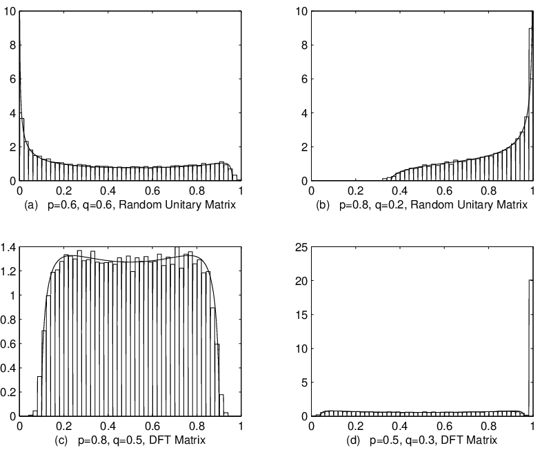
Refer to caption — Figure 1: Empirical eigenvalue distribution plotted against continuous part of asymptotic distribution. In plots (a) and (b) the matrices are submatrices of a random unitary matrix with Haar distribution. In plots (c) and (d) the matrices are submatrices of the DFT matrix. In each case, the original matrix dimension was $100/(1-\max(p,q))$ , so that the submatrices all had expected dimensions $100\times 100$ . Each random matrix was realized $100$ times.

Note that $r_{-}=0$ only when $p=q$ ; that is, when $F_{\Omega_{n}T_{n}}F_{\Omega_{n}T_{n}}^{*}$ or $\mathcal{U}_{\Omega_{n}T_{n}}\mathcal{U}_{\Omega_{n}T_{n}}^{*}$ is asymptotically square. Therefore, when $p\neq q$ the support of the limiting distribution begins at $r_{-}>0$ . Also, $r_{+}=1$ only when $p+q=1$ , so when $p+q\neq 1$ there is a gap in the support of the limiting distribution from $r_{+}$ to $1$ . When $r_{-}\neq 0$ and $r_{+}\neq 1$ the continuous part of the measure begins at $r_{-}$ and makes an arc ending at $r_{+}$ . When $r_{-}=0$ or $r_{+}=1$ , the continuous part of (21) tends to $\infty$ as $x\rightarrow 0$ or $x\rightarrow 1$ . When $p+q<1$ there is a point mass of measure $1-(p+q)$ at $1$ , and when $p+q>1$ , the support stops at $r_{+}$ and there is no point mass at $1$ . In Figure 1 the continuous part of the asymptotic distribution is plotted against empirical values for several parameter pairs $p$ and $q$ .

We discuss the relationship between Theorem 3.1 and uncertainty principles and other areas before turning to the proof. We focus first on the DFT case and assume that the dimension is $n$ . The norm of a DFT matrix with a set of rows and columns removed equals $1$ if and only if there exists a vector with time support corresponding to the remaining columns and frequency support corresponding to the remaining rows. That is, denoting $Fx=\hat{x}$ , in the notation of this paper, $\|F_{\Omega T}\|=1$ if and only if there exists $x\in\mathbb{C}^{n}$ such that $\textnormal{supp}(x)\subset T$ and $\textnormal{supp}(\hat{x})\subset\Omega$ . One is then interested in determining conditions on the cardinality of $|\Omega|$ and $|T|$ such that $\|F_{\Omega T}\|<1$ , where generally at least one set is random and a statement is made in some probabilistic form. This non-asymptotic question has been studied intensively over the last ten years. Recent results and a general discussion can be found in [14]. While Theorem 3.1 does not assert the non-existence of any vectors, it does state when certain vectors do exist and sheds light on one of the main theorems in this area, namely that of Tao.

Theorem 3.2 (Tao, [13])

If $n$ is prime and $|\Omega|+|T|<n$ , then $\|F_{\Omega T}\|<1$ .

Note that since Tao’s theorem requires $n$ to be prime, it precludes the case that $\frac{|\Omega|}{n}+\frac{|T|}{n}=1$ . Theorem 3.1 says that if $\frac{|\Omega_{n}|}{n}+\frac{|T_{n}|}{n}\rightarrow 1$ , then $\|F_{\Omega_{n}T_{n}}\|$ converges almost surely to $1$ , and in fact this also holds for random unitary matrices $\mathcal{U}_{\Omega_{n}T_{n}}\mathcal{U}_{\Omega_{n}T_{n}}^{*}$ . Almost sure convergence and the existence of infinitely many primes imply that for all $\epsilon_{1},\epsilon_{2}>0$ , there exists a prime $n$ and sets $\Omega_{n},T_{n}\subset\{1,...,n\}$ such that $\frac{|\Omega_{n}|}{n}+\frac{|T_{n}|}{n}<1+\epsilon_{1}$ and $\|F_{\Omega_{n}T_{n}}\|>1-\epsilon_{2}$ . In fact, the proportion of subsets for which $\|F_{\Omega_{n}T_{n}}\|<1-\epsilon_{2}$ converges to $0$ as $n\rightarrow\infty$ . Moreover, as $n$ increases, the Haar measure of the set of unitary matrices $U$ such that $\|U_{\Omega_{n}T_{n}}\|>1-\epsilon_{2}$ for random sets satisfying $\frac{|\Omega_{n}|}{n}+\frac{|T_{n}|}{n}<1+\epsilon_{1}$ also converges to $1$ .

A further area of interest is the smallest eigenvalue of $F_{\Omega_{n}T_{n}}F_{\Omega_{n}T_{n}}^{*}$ or $\mathcal{U}_{\Omega_{n}T_{n}}\mathcal{U}_{\Omega_{n}T_{n}}^{*}$ ; in particular, one would like to bound the smallest eigenvalue away from $0$ . See [12] for recent results in the setting of independent matrix entries. While Theorem 3.1 does not make any statement on when the smallest eigenvalue is strictly positive, it does say that if $\frac{|\Omega_{n}|}{|Tn|}\rightarrow 1$ , then the smallest eigenvalue of $F_{\Omega_{n}T_{n}}F_{\Omega_{n}T_{n}}^{*}$ and $\mathcal{U}_{\Omega_{n}T_{n}}\mathcal{U}_{\Omega_{n}T_{n}}^{*}$ converge to $0$ . This corresponds to the behavior of square matrices with independent entries, though in that case non-asymptotic bounds away from $0$ exist [12].

Theorem 3.1 and some numerical experiments suggest the obvious conjecture that the largest and smallest eigenvalues converge to the edge of the limiting support. This would imply that Tao’s result gives the general uncertainty principle behavior for DFT and random unitary matrices, and that the submatrices that do not have this behavior have measure zero asymptotically. As was the case for the Wigner and Wishart distributions, we hope that the limiting empirical distribution is helpful in determining the behavior of the extremal eigenvalues.

We note, lastly, that a potential further step in this direction is restricted isometry properties. Here one set, say $T_{n}$ , is taken at random and one seeks to bound the extremal eigenvalues of $F_{\Omega_{n}T_{n}}F_{\Omega_{n}T_{n}}^{*}$ or $\mathcal{U}_{\Omega_{n}T_{n}}\mathcal{U}_{\Omega_{n}T_{n}}^{*}$ when $\Omega_{n}$ ranges over all subsets of certain cardinality. This property of random matrices is central to compressed sensing and has received enormous attention in recent years; see [4] for a recent overview.

Proof [Proof of Theorem 3.1.] We give the proof using the notation for the DFT case, but the two are identical. We begin by working with $P_{n}F_{n}Q_{n}F_{n}^{*}P_{n}$ , where $P_{n}$ and $Q_{n}$ are a sequence of independent Bernoulli diagonal projection matrices, as defined earlier, with expected traces $1-p\in(0,1)$ and $1-q\in(0,1)$ respectively. By Proposition 2.6 we have

|\frac{1}{n}\sum_{i=1}^{n}\frac{1}{1+z\lambda_{i}}-\eta_{p,q}(z)|\stackrel{{\scriptstyle a.s.}}{{\longrightarrow}}0

(22)

for all $z\in\mathbb{C}^{+}$ . By applying this to $-\frac{1}{z}$ , multiplying both terms in (22) by $-\frac{1}{z}$ and using equation (3), we obtain

|\frac{1}{n}\sum_{i=1}^{n}\frac{1}{z-\lambda_{i}}-m_{p,q}(z)|\stackrel{{\scriptstyle a.s.}}{{\longrightarrow}}0.

Thus, the random measures induced by the eigenvalues at each dimension $n$ converge almost surely to the probability measure corresponding to $m_{p,q}$ [1] (Theorem 2.4.4(c) in [1] also holds for almost sure convergence). By equation (3) the limiting Stieltjes transform is

	$\displaystyle m_{p,q}(z)$	$\displaystyle=$	$\displaystyle\frac{-1}{z}\cdot\frac{1-(p+q)\frac{1}{z}+\sqrt{1+(2(p+q)-4pq)(\frac{-1}{z})+(p-q)^{2}(\frac{1}{z})^{2}}}{2(1-\frac{1}{z})}$
		$\displaystyle=$	$\displaystyle\frac{1-(p+q)\frac{1}{z}+\sqrt{1-(2(p+q)-4pq)\frac{1}{z}+(p-q)^{2}\frac{1}{z^{2}}}}{2(1-z)},$

and we are interested in the inverse Stieltjes transform

\lim_{\omega\rightarrow 0^{+}}\frac{1}{\pi}\Im\;m_{p,q}(x+i\omega).

$m_{p,q}(x+i\omega)$ is a continuous function of both $x$ and $\omega$ for $x\in(0,1)$ . Thus, using equation (1) for $x\in(0,1)$ ,

	$\displaystyle f_{p,q}(x)$	$\displaystyle=$	$\displaystyle\frac{1}{\pi}\Im\;\frac{1-(p+q)\frac{1}{x}+\sqrt{1-(2(p+q)-4pq)\frac{1}{x}+(p-q)^{2}\frac{1}{x^{2}}}}{2(1-x)}$		(23)
		$\displaystyle=$	$\displaystyle\Im\;\frac{\sqrt{1-(2(p+q)-4pq)\frac{1}{x}+(p-q)^{2}\frac{1}{x^{2}}}}{2\pi(1-x)}.$		(23)

Imitating Marčenko and Pastur [10], we denote the roots of the equation $x^{2}-(2(p+q)-4pq)x+(p-q)^{2}=0$ by $r_{-}$ and $r_{+}$ . These values are

$\displaystyle r_{-}$	$\displaystyle=$	$\displaystyle\frac{(2(p+q)-4pq)-\sqrt{(2(p+q)-4pq)^{2}-4(p-q)^{2}}}{2}$
	$\displaystyle=$	$\displaystyle\frac{(2(p+q)-4pq)-2\sqrt{(p+q-2pq-(p-q))(p+q-2pq+(p-q))}}{2}$
	$\displaystyle=$	$\displaystyle\frac{(2(p+q)-4pq)-2\sqrt{(2q(1-p))(2p(1-q))}}{2}$
	$\displaystyle=$	$\displaystyle p(1-q)+q(1-p)-2\sqrt{p(1-q)q(1-p)}$
	$\displaystyle=$	$\displaystyle(\sqrt{p(1-q)}-\sqrt{q(1-p)})^{2}$

and $r_{+}=(\sqrt{p(1-q)}+\sqrt{q(1-p)})^{2}$ , as defined in the statement of the theorem. For $x\in(0,1)$ equation (23) is now

$\displaystyle f_{PFQF^{*}P}(x)$	$\displaystyle=$	$\displaystyle\Im\;\frac{\sqrt{1-(2(p+q)-4pq)\frac{1}{x}+(p-q)^{2}\frac{1}{x^{2}}}}{2\pi(1-x)}$	(24)
	$\displaystyle=$	$\displaystyle\Im\frac{\sqrt{(1-\frac{r_{-}}{x})(1-\frac{r_{+}}{x})}}{2\pi(1-x)}$
	$\displaystyle=$	$\displaystyle\frac{\sqrt{(1-\frac{r_{-}}{x})(\frac{r_{+}}{x}-1)}}{2\pi(1-x)}\cdot I_{[r_{-},r_{+}]}(x).$

We now determine the density at $x=0$ , for which we need to find the asymptotic proportion of zero eigenvalues of $P_{n}F_{n}Q_{n}F_{n}^{*}P_{n}$ or $P_{n}\mathcal{U}_{n}Q_{n}\mathcal{U}_{n}^{*}P_{n}$ . This proportion is given by $\lim_{r\rightarrow\infty}\eta_{p,q}(r)$ , since the latter quantity gives the measure of the set ${0}$ with respect to the measure $f_{p,q}$ . We have

$\displaystyle\lim_{r\rightarrow\infty}\eta_{p,q}(r)$	$\displaystyle=$	$\displaystyle\lim_{r\rightarrow\infty}\frac{1+(p+q)r+\sqrt{1+(2(p+q)-4pq)r+(p-q)^{2}r^{2}}}{2(1+r)}$	(25)
	$\displaystyle=$	$\displaystyle\frac{(p+q)+\|p-q\|}{2}$
	$\displaystyle=$	$\displaystyle\max(p,q).$

Lastly, we investigate the point $x=1$ . We denote by $\mu(1)$ the measure of the set $\{1\}$ with respect to the limiting distribution. Let $X$ denote the random variable of the eigenvalues. We first must address the convergence of $\sum_{k=0}^{\infty}(-z)^{k}\mathbb{E}X^{k}$ . If $p+q\neq 1$ and $p\neq q$ , then $0<r_{-}$ and $r_{+}<1$ , and

	$\displaystyle\mathbb{E}X^{k}$	$\displaystyle\leq$	$\displaystyle\\|\frac{\sqrt{(1-\frac{r_{-}}{x})(\frac{r_{+}}{x}-1)}}{2\pi(1-x)}I_{[r_{-},r_{+}]}\\|_{\infty}\cdot\int_{0}^{r_{+}}r_{+}^{k}dx+\mu(1)$
		$\displaystyle=$	$\displaystyle\\|\frac{\sqrt{(1-\frac{r_{-}}{x})(\frac{r_{+}}{x}-1)}}{2\pi(1-x)}I_{[r_{-},r_{+}]}\\|_{\infty}\cdot r_{+}^{k+1}+\mu(1).$

If $p+q\neq 1$ and $p=q$ , which implies $r_{-}=0$ , then we pick a small $\epsilon$ and have

	$\displaystyle\mathbb{E}X^{k}$	$\displaystyle\leq$	$\displaystyle\int_{0}^{\epsilon}\epsilon^{k}\frac{\sqrt{(1-\frac{r_{-}}{x})(\frac{r_{+}}{x}-1)}}{2\pi(1-x)}dx$
			$\displaystyle+\\|\frac{\sqrt{(1-\frac{r_{-}}{x})(\frac{r_{+}}{x}-1)}}{2\pi(1-x)}I_{[\epsilon,r_{+}]}\\|_{\infty}\cdot\int_{0}^{r_{+}}r_{+}^{k}dx+\mu(1).$

When $p+q=1$ and when $z$ belongs to a region of convergence to be determined shortly, equation (2) implies

$\displaystyle\eta_{p,q}(z)$	$\displaystyle=$	$\displaystyle\sum_{k=0}^{\infty}(-z)^{k}\mathbb{E}X^{k}$	(26)
	$\displaystyle=$	$\displaystyle\sum_{k=0}^{\infty}(-z)^{k}\int_{r_{-}}^{r_{+}}x^{k}\frac{\sqrt{(1-\frac{r_{-}}{x})(\frac{r_{+}}{x}-1)}}{2\pi(1-x)}dx+\sum_{k=0}^{\infty}\mu(1)(-z)^{k}$
	$\displaystyle=$	$\displaystyle\sum_{k=0}^{\infty}(-z)^{k}\int_{r_{-}}^{r_{+}}x^{k}\frac{\sqrt{(1-\frac{r_{-}}{x})(\frac{r_{+}}{x}-1)}}{2\pi(1-x)}dx+\frac{\mu(1)}{1+z}.$

Since we have assumed that neither $p$ or $q$ equals $1$ or $0$ , we have $r_{-}<1$ . We show that the sum on the left side of equation (26) converges for $|z|\leq 1/r_{-}$ . We define $\lfloor k\rfloor_{e}=\Big\{\begin{array}[]{ll}k&k\;\textnormal{even}\\ k-1&k\;\textnormal{odd}\end{array}$ .

$\displaystyle\left\|\sum_{k=0}^{\infty}(-z)^{k}\int_{r_{-}}^{1}x^{k}\frac{\sqrt{(1-\frac{r_{-}}{x})(\frac{r_{+}}{x}-1)}}{2\pi(1-x)}dx\right\|$			(27)
	$\displaystyle\leq$	$\displaystyle\sum_{k=0}^{2}\|z\|^{k}\mathbb{E}X^{k}+\sum_{k=3}^{\infty}\|z\|^{k}\int_{r_{-}}^{1}x^{k}\frac{\sqrt{\frac{1}{x}-1}}{2\pi(1-x)}dx$
	$\displaystyle=$	$\displaystyle\sum_{k=0}^{2}\|z\|^{k}\mathbb{E}X^{k}+\sum_{k=3}^{\infty}\|z\|^{k}\int_{r_{-}}^{1}x^{k}\frac{\sqrt{\frac{1-x}{x}}}{2\pi(1-x)}dx$
	$\displaystyle=$	$\displaystyle\sum_{k=0}^{2}\|z\|^{k}\mathbb{E}X^{k}+\frac{1}{2\pi}\sum_{k=3}^{\infty}\|z\|^{k}\int_{r_{-}}^{1}x^{k-1/2}(1-x)^{-1/2}dx$
	$\displaystyle\leq$	$\displaystyle\sum_{k=0}^{2}\|z\|^{k}\mathbb{E}X^{k}+\frac{\|z\|}{2\pi}\sum_{k=2}^{\infty}\|z\|^{k}\int_{r_{-}}^{1}x^{k}(1-x)^{-1/2}dx$
	$\displaystyle\leq$	$\displaystyle\sum_{k=0}^{2}\|z\|^{k}\mathbb{E}X^{k}+\frac{\|z\|}{2\pi}\sum_{k=2}^{\infty}\|z\|^{k}\int_{r_{-}}^{1}x^{\lfloor k\rfloor_{e}}(1-x)^{-1/2}dx$
	$\displaystyle=$	$\displaystyle\sum_{k=0}^{2}\|z\|^{k}\mathbb{E}X^{k}+\frac{\|z\|}{2\pi}\sum_{k=2}^{\infty}\|z\|^{k}2(1-r_{-})^{1/2}\sum_{j=0}^{\lfloor k\rfloor_{e}}\frac{(-1)^{j}\binom{\lfloor k\rfloor_{e}}{j}(1-r_{-})^{\lfloor k\rfloor_{e}-j}}{2(\lfloor k\rfloor_{e}-j)+3}.$

The integral in line (27) is given by equation 2.221 in [8]. One may verify that

\frac{\binom{n}{k}(1-r_{+})^{n-k}}{2(n-k)+3}-\frac{\binom{n}{k-1}(1-r_{+})^{n-k+1}}{2(n-k+1)+3}<\binom{n}{k}(1-r_{+})^{n-k}-\binom{n}{k-1}(1-r_{+})^{n-k+1},

so that

\sum_{j=0}^{\lfloor k\rfloor_{e}}\frac{(-1)^{j}\binom{\lfloor k\rfloor_{e}}{j}(1-r_{-})^{\lfloor k\rfloor_{e}-j}}{2(\lfloor k\rfloor_{e}-j)+3}\leq\sum_{j=0}^{\lfloor k\rfloor_{e}}(-1)^{j}\binom{\lfloor k\rfloor_{e}}{j}(1-r_{-})^{\lfloor k\rfloor_{e}-j}=r_{-}^{\lfloor k\rfloor_{e}}.

Thus

(\ref{trickyintegral})\leq\sum_{k=0}^{2}|z|^{k}\mathbb{E}X^{k}+\frac{|z|}{2\pi}(1-r_{-})^{1/2}\sum_{k=2}^{\infty}|z|^{-k}r_{-}^{\lfloor k\rfloor_{e}},

which converges for all $|z|<1/r_{-}$ . This gives

\mu(1)=(1+z)\eta_{p,q}(z)-(1+z)\sum_{k=0}^{\infty}z^{k}\int_{r_{-}}^{r_{+}}x^{k}\frac{\sqrt{(1-\frac{r_{-}}{x})(\frac{r_{+}}{x}-1)}}{2\pi(1-x)}dx,

(28)

where equation (28) holds for all values $|z|<1$ , and the sum on the right side of equation (28) remains finite as $z\rightarrow-1$ . Convergence of the necessary sums and integrals is now established for all $p,q\in(0,1)$ . Using the equation for $\eta_{p,q}(z)$ from Proposition 2.6,

(1+z)\eta_{p,q}(z)=\frac{1+(p+q)z+\sqrt{1+(2(p+q)-4pq)z+((p+q)^{2}-4pq)z^{2}}}{2}.

Allowing $z\rightarrow-1$ , we have

	$\displaystyle\mu(1)$	$\displaystyle=$	$\displaystyle\frac{1-(p+q)+\sqrt{(1-(p+q))^{2}}}{2}$		(29)
		$\displaystyle=$	$\displaystyle\frac{1-(p+q)+\|1-(p+q)\|}{2}.$		(29)

When $p+q\geq 1$ , equation (29) is equal to $0$ , and when $p+q<0$ , equation (29) is equal to $1-\min(p,q)$ . From equations (25) and (29), it follows that when $p+q>1$

\int_{r_{-}}^{r_{+}}\frac{\sqrt{(1-\frac{r_{-}}{x})(\frac{r_{+}}{x}-1)}}{2\pi(1-x)}dx=1-\max(p,q),

and when $p+q\leq 1$ ,

\int_{r_{-}}^{r_{+}}\frac{\sqrt{(1-\frac{r_{-}}{x})(\frac{r_{+}}{x}-1)}}{2\pi(1-x)}dx=\min(p,q).

Now it only remains to remove the point mass at $0$ and normalize the distribution by $1/(1-\max(p,q))$ . x

For the following corollary we define the $n$ singular values of the matrix $P_{n}F_{n}Q_{n}$ to be the (positive) square roots of the $n$ eigenvalues of the matrix $P_{n}F_{n}Q_{n}F_{n}^{*}P_{n}$ . We thus have the following limiting distribution for the singular values of $P_{n}F_{n}Q_{n}$ .

Corollary 3.3

For $i=1,...,n$ let $i$ be contained in $\Omega_{n}$ independently with probability $(1-q)$ and, also independently, let $i$ be included in $T_{n}$ with probability $(1-p)$ . Then the empirical distributions of the $\min(|T_{n}|,|\Omega_{n}|)$ largest singular values of $F_{\Omega_{n}T_{n}}$ and $\mathcal{U}_{\Omega_{n}T_{n}}$ converge almost surely to

f^{s}_{p,q}(x)=\frac{\sqrt{x^{2}(1-\frac{r^{s}_{-}}{x})(\frac{r^{s}_{+}}{x}-1)}}{2\pi(1-x^{2})(1-\max(p,q))}\cdot I_{(r^{s}_{-},r^{s}_{+})}(x)+\frac{\max(0,1-(p+q))}{1-\max(p,q)}\cdot\delta(x-1)

where

r^{s}_{-}=|\sqrt{p(1-q)}-\sqrt{q(1-p)}|

and

r^{s}_{+}=\sqrt{p(1-q)}+\sqrt{q(1-p)}.

Proof The measures for the singular values $0$ and $1$ are the same as the eigenvalues $0$ and $1$ of the previous theorem. Also, the continuous part of the measure will clearly have support $[r^{s}_{-},r^{s}_{+}]=[\sqrt{r_{-}},\sqrt{r_{+}}]$ . Using equation (24), we have

$\displaystyle f^{s}_{p,q}(x)$	$\displaystyle=$	$\displaystyle 2xf_{p,q}(x^{2})$
	$\displaystyle=$	$\displaystyle\Im\;2x\frac{\sqrt{(1-\frac{r_{-}}{x^{2}})(1-\frac{r_{+}}{x^{2}})}}{2\pi(1-x^{2})}$
	$\displaystyle=$	$\displaystyle\Im\;x\frac{\sqrt{(1-\frac{r_{-}}{x^{2}})(\frac{r_{+}}{x^{2}}-1)}}{\pi(1-x^{2})}$
	$\displaystyle=$	$\displaystyle\frac{\sqrt{x^{2}(1-\frac{r_{-}}{x^{2}})(\frac{r_{+}}{x^{2}}-1)}}{\pi(1-x^{2})}\cdot I_{[\sqrt{r_{-}},\sqrt{r_{+}}]}(x).$

Acknowledgement The author thanks Roland Speicher, Walid Hachem, Antonia Tulino and Sergio Verdú for helpful discussions and comments.

References

[1] G. Anderson, A. Guionnet, and O. Zeitouni, An introduction to random matrices, Cambridge University Press, Cambridge, 2009.
[2] Z. D. Bai and Y. Q. Yin, Necessary and sufficient conditions for almost sure convergence of the largest eigenvalue of a Wigner matrix, Ann. Probab. 16 (1988), no. 4, 1729–1741.
[3] Z. D. Bai and Y. Q. Yin, Limit of the smallest eigenvalue of a large-dimensional sample covariance matrix, Ann. Probab. 21 (1993), no. 3, 1275–1294.
[4] Emmanuel J. Candès, Compressive sampling, International Congress of Mathematicians. Vol. III, Eur. Math. Soc., Zürich, 2006, pp. 1433–1452.
[5] A.Yu. Garnaev and E.D. Gluskin, On widths of the Euclidean ball., Sov. Math., Dokl. 30 (1984), 200–204 (English. Russian original).
[6] Stuart Geman, A limit theorem for the norm of random matrices, Ann. Probab. 8 (1980), no. 2, 252–261.
[7] E.D. Gluskin, Norms of random matrices and widths of finite-dimensional sets., Math. USSR, Sb. 48 (1984), 173–182 (English).
[8] I.S. Gradshteyn and I.M. Ryzhik, Table of integrals, series, and products, Academic Press, New York, 2000.
[9] Ulf Grenander and Jack W. Silverstein, Spectral analysis of networks with random topologies, SIAM J. Appl. Math. 32 (1977), no. 2, 499–519.
[10] V. A. Marčenko and L. A. Pastur, Distribution of eigenvalues in certain sets of random matrices, Mat. Sb. (N.S.) 72 (114) (1967), 507–536.
[11] Dénes Petz and Júlia Réffy, Large deviation for the empirical eigenvalue density of truncated Haar unitary matrices., Probab. Theory Relat. Fields 133 (2005), no. 2, 175–189 (English).
[12] M. Rudelson and R. Vershynin, The Littlewood-Offord problem and invertibility of random matrices, Adv. Math. 218 (2008), no. 2, 600–633.
[13] T. Tao, An uncertainty principle for cyclic groups of prime order, Math. Res. Lett. 12 (2005), no. 1, 121–127.
[14] Joel A Tropp, On the linear independence of spikes and sines, Journal of Fourier Analysis and Applications 14 (2008), no. 5, 838–858.
[15] A. Tulino, G. Caire, S. Shamai, and S. Verdú, Capacity of channels with frequency-selective and time-selective fading, IEEE Trans. Information Theory (2010), to appear.
[16] A. Tulino and S. Verdú, Random matrices and wireless communications, Foundations and Trends in Information Theory 1 (June 2004), no. 1.
[17] A. Tulino, S. Verdú, G. Caire, and S. Shamai, Capacity of the gaussian erasure channel, Preprint, Technion CCIT no. 655 (2007), http://www3.ee.technion.ac.il/ccit/info/Publication/Scientific_e.asps.
[18] Eugene P. Wigner, Characteristic vectors of bordered matrices with infinite dimensions, Ann. of Math. (2) 62 (1955), 548–564.
[19] Eugene P. Wigner, On the distribution of the roots of certain symmetric matrices, Ann. of Math. (2) 67 (1958), 325–327.
[20] J. Wishart, The generalized product moment distribution in samples from a normal multivariate population, Biometrika 20A (1928), 32–52.
[21] Y. Q. Yin, Z. D. Bai, and P. R. Krishnaiah, On the limit of the largest eigenvalue of the large-dimensional sample covariance matrix, Probab. Theory Related Fields 78 (1988), no. 4, 509–521.
[22] Karol Życzkowski and Hans-Jürgen Sommers, Truncations of random unitary matrices, J. Phys. A 33 (2000), no. 10, 2045–2057.

$\displaystyle\mathbb{E}_{\bar{P},\mathcal{U}}\|T_{i,j}\|^{m}$
	$\displaystyle=$	$\displaystyle\mathbb{E}[\|T_{i,j}\|^{m}\big\|\;\\|\vec{u}_{i}\\|_{\infty}\leq M\;\textnormal{ and }\\|\vec{u}_{j}\\|_{\infty}\leq M]\cdot\mathbb{P}\Big(\big\|\;\\|\vec{u}_{i}\\|_{\infty}\leq M\;\textnormal{ and }\\|\vec{u}_{j}\\|_{\infty}\leq M\Big)$
	$\displaystyle+$	$\displaystyle\mathbb{E}[\|T_{i,j}\|^{m}\|\big\|\;\\|\vec{u}_{i}\\|_{\infty}>M\;\textnormal{ or }\\|\vec{u}_{j}\\|_{\infty}>M]\cdot\mathbb{P}\Big(\big\|\;\\|\vec{u}_{i}\\|_{\infty}>M\;\textnormal{ or }\\|\vec{u}_{j}\\|_{\infty}>M\Big)$
	$\displaystyle\leq$	$\displaystyle\mathbb{E}[\|T_{i,j}\|^{m}\|\big\|\;\\|\vec{u}_{i}\\|_{\infty}\leq M\;\textnormal{ and }\\|\vec{u}_{j}\\|_{\infty}\leq M]+e^{-cn}.$

	$\displaystyle W^{}A^{-1}_{i^{}}W$	$\displaystyle=$	$\displaystyle V^{}P(I+zPVQV^{}P-zQ_{(i^{},i^{})}w_{i}^{}w_{i^{}}^{*})^{-1}PV$
		$\displaystyle=$	$\displaystyle V^{}P\sum_{k=0}^{\infty}(-z)^{k}(PVQV^{}P-zQ_{(i^{},i^{})}w_{i}^{}w_{i^{}}^{*})^{k}PV.$

$\displaystyle V^{}P\sum_{k=0}^{K}(-z)^{k}(PVQV^{}P-zQ_{(i^{},i^{})}w_{i}^{}w_{i^{}}^{*})^{k}PV$
	$\displaystyle=$	$\displaystyle\sum_{k=0}^{K}(-z)^{k}V^{}P[PV\tilde{Q}V^{}P+(1-q)P]^{k}PV$
	$\displaystyle=$	$\displaystyle\sum_{k=0}^{K}(-z)^{k}\sum_{j=0}^{k}\binom{k}{j}(1-q)^{j}V^{}P[PV\tilde{Q}V^{}P]^{k-j}P^{j}PV$
	$\displaystyle=$	$\displaystyle\sum_{k=0}^{K}(-z)^{k}\sum_{j=0}^{k}\binom{k}{j}(1-q)^{j}V^{}P[V\tilde{Q}V^{}P]^{k-j}V.$

	$\displaystyle V^{}P[V\tilde{Q}V^{}P]^{k}V$	$\displaystyle=$	$\displaystyle V^{}(\tilde{P}+(1-p)I)[V\tilde{Q}V^{}(\tilde{P}+(1-p)I)]^{k}V$
		$\displaystyle=$	$\displaystyle\sum_{\alpha}(1-p)^{k+1-\|\alpha\|}V^{}\tilde{P}^{\alpha_{0}}V\tilde{Q}V^{}\tilde{P}^{\alpha_{1}}V\tilde{Q}\cdots\tilde{P}^{\alpha_{k}}V$

$\displaystyle zQ_{i,i}w_{i}w_{i}^{}(I+zPVQV^{}P)^{-1}$
	$\displaystyle=$	$\displaystyle zQ_{i,i}w_{i}w_{i}^{}A_{i}^{-1}-\frac{z^{2}Q^{2}_{i,i}w_{i}w_{i}^{}}{1+zQ_{i,i}w_{i}^{}A_{i}^{-1}w_{i}}A_{i}^{-1}w_{i}w_{i}^{}A_{i}^{-1}$
	$\displaystyle=$	$\displaystyle zQ_{i,i}w_{i}w_{i}^{}A_{i}^{-1}(1-\frac{zQ_{i,i}w_{i}^{}A_{i}^{-1}w_{i}}{1+zQ_{i,i}w_{i}^{*}A_{i}^{-1}w_{i}})$
	$\displaystyle=$	$\displaystyle\frac{zQ_{i,i}}{1+zQ_{i,i}w_{i}^{}A_{i}^{-1}w_{i}}w_{i}w_{i}^{}A_{i}^{-1}.$

Limiting Empirical Singular Value Distribution of Restrictions of Unitary Matrices

Abstract

1 Introduction

1.1 Notation

Definition 1.1

Definition 1.2

Note 1.3

Note 1.4

2 The Stieltjes and η\eta Transforms

Lemma 2.1

Theorem 2.2 (Main Theorem in [5])

Lemma 2.3

Lemma 2.4

Lemma 2.5

Proposition 2.6

3 Limiting Empirical Distributions

Theorem 3.1

Theorem 3.2 (Tao, [13])

Corollary 3.3

References

2 The Stieltjes and $\eta$ Transforms