Quantum spin metal state on a decorated honeycomb lattice

Quantum spin liquids  [1, 2, 3, 4, 5] present very interesting examples of strongly correlated phases of matter which do not follow the classical Landau route: no local order parameter is formed while the entropy vanishes at zero temperature. Although quite a number of different proposals for the realization of spin liquid states are available, and many interesting results were obtained numerically, see e.g. [4], the progress in analitical theory was hindered for a long time due to the absense of an appropriate quantum spin model exactly solvable in more than one spatial dimension. Seminal results due to A. Kitaev [6] may pave the way to fill this gap. Kitaev proposed spin-$\frac{1}{2}$ model with anisotropic nearest-neighbour spin interactions $J_{\alpha}\sigma_{i}^{\alpha}\sigma_{j}^{\alpha}$ (where $\alpha=x,y,z$) on the honeycomb lattice. The model allows for the two-dimensional generalization of the Jordan-Wigner spin-to-fermion transformation and can be thus exactly diagonalized. Kitaev model realizes different phases as its ground-states, the most interesting of them corresponds to the region around symmetric point $J_{x}=J_{y}=J_{z}=J^{\prime}$. The excitations above this ground-state constitute a single branch of massless Dirac fermions (Kitaev presents them in terms of Majorana fermions those spectrum contains two symmetric conical points). Thus the Kitaev honeycomb model presents exactly solvable case of the critical QSL. Although long-range spin correlations vanish in this model presisely due to its integrability [7], it presents valuable starting point for the construction of analitically controllable theories possessing long-range spin correlations.

Still, here we discuss another extension of the model [6]: it is interesting to find exact realizations of other types of QSLs, the one with gapful excitation spectrum, and the one with a whole surface of gapless excitations [8]. Gapful QSL was recently found by Yao and Kivelson [9]. They proposed specific generalization of the Kitaev model, where each site of the honeycomb lattice is replaced by a triangle (we will call it, for brevity, ”3-12 lattice”), with internal coupling strengths equal to $J$ and inter-triangle couplings equal to $J^{\prime}$. Topologically equivalent structure of such a lattice is shown in Fig. 1. Yao-Kivelson model is exactly solvable and contains a critical point at $g\equiv J^{\prime}/J=\sqrt{3}$. At $g=\sqrt{3}$ the excitation spectrum has single low-energy branch of Dirac fermions, like the original Kitaev model, whereas at any other $g$ the excitation spectrum is gapful. Yao and Kivelson have shown that the ground state at $g<\sqrt{3}$ is a topologically nontrivial chiral spin liquid with Chern number $\mathrm{C}=\pm 1$, whereas $g>\sqrt{3}$ phase is topologically trivial, with $\mathrm{C}=0$. Exactly solvable QSL model of spin-metal type with spins-$\frac{3}{2}$ was proposed by Yao, Zhang and Kivelson [10]. In the present Letter we take a different route: we show that slight modification of the Hamiltonian of spin-$\frac{1}{2}$ Yao-Kivelson model on the 3-12 lattice leads to the spin-metal QSL with a pseudo-Fermi-circle. Similar approach was proposed recently in Ref. [11] where QSL with pseudo-Fermi-line was found in the spin-$\frac{1}{2}$ model on a decorated square lattice. Apart from another lattice studied, our study differs from [11] in two respects: i) our Fermi-liquid-like ground state is the result of spontaneous symmetry breaking leading to a ”chiral antiferromagnet” ordering defined in terms of 3-spin products, ii) we present analitic results for heat capacity and dynamic spin susceptibility in the limit of small Fermi-surface size.

We consider the Hamiltonian:

Here $T_{p}=\sigma_{ia}^{x}\sigma_{jb}^{y}\sigma_{kc}^{z}$ is the three-spin ”exchange” operator corresponding to the $p$-th triangle. We take $J_{x,y,z}=J,$ $J_{x^{\prime},y^{\prime},z^{\prime}}=J^{\prime}$ and without loss of generality assume $~J,~J^{\prime}>0$. Unit vectors $\mathbf{n}_{l}$ are parallel to $x$, $y$ and $z$ axis for the corresponding links $x$, $x^{\prime}$, etc. Eq. (1) reduces to the original Hamiltonian of Ref. [9] at $\lambda=0$. This spin Hamiltonian is rather special, since it posesses large number of independent integrals of motion, so called fluxes defined as $W_{p}=\prod_{s=1}^{n}\sigma_{j_{s}}^{\alpha}\sigma_{j_{s-1}}^{\alpha}$, where $j_{0},~j_{1},~...,~j_{n}=j_{0}$ defines a minimal close loop on the lattice. All $W_{p}$ commute with Hamiltonian and with each other and divide total Hilbert space into sectors, corresponding to different sets of $W_{p}$ eigenvalues.

Hamiltonian (1) can be diagonalized by means of Kitaev representation of spins via 4 Majorana fermions: $\sigma_{i}^{\alpha}=ic_{i}c_{i}^{\alpha}$, where four Majorana operators $c_{i},c_{i}^{x},c_{i}^{y},c_{i}^{z}$ are defined on each site of the lattice and satisfy anticommutation relations $\left\{c_{i}^{\alpha},c_{j}^{\beta}\right\}=2\delta_{ij}\delta_{\alpha\beta}$. This way, each spin (2-dim Hilbert space) is represented by four Majoranas  (4-dim Hilbert space). This is a representation in the extended Hilbert space; all physical states should satisfy the constraint: $D_{i}\left|\Psi_{phys}\right\rangle=\left|\Psi_{phys}\right\rangle$ for any lattice site $i$, where $D_{i}=c_{i}c_{i}^{x}c_{i}^{y}c_{i}^{z}$. Operators $D_{i}$ is the gauge transformation operator for the group $\mathcal{Z}_{2}$. Hamiltonian (1), extended to the Hilbert space of Majorana fermions, reads ($u_{ij}=ic_{i}^{\alpha}c_{j}^{\alpha}$):

with $t_{p}=u_{ab}u_{bc}u_{ca}$. Note, that $[u_{ij},H]=0$ and $u_{ij}^{2}=1$ . These integrals of motion are gauge-dependent; they are related to the gauge-invariant fluxes $W_{p}=\prod_{s=1}^{n}\left(-iu_{j_{s}j_{s-1}}\right)$. There are two types of $W_{p}$  : 1) fluxes, corresponding to the triangular loops $W_{p}^{(3)}=\pm i$, and 2) fluxes $W_{p}^{(12)}=\pm 1$ corresponding to the dodecagon loops. They respond differently to the time reversal transformation: ${\mathcal{\hat{T}}}W_{p}^{(12)}=W_{p}^{(12)}$, but ${\mathcal{\hat{T}}}W_{p}^{(3)}=-W_{p}^{(3)}$. It was shown in Ref. [12] that the ground state of Hamiltonian (1) with $\lambda=0$ corresponds to all $W_{p}^{(12)}=-1$ and all $W_{p}^{(3)}~$ are equal (either to $i$, or to $-i$) ; these two global eigenstates are related by the $\mathcal{\hat{T}}$ inversion. We show now that in some range of couplings $J,J^{\prime}$ even very small $\lambda$ stabilizes another type of the ground state, with variables $W_{p}^{(3)}=\pm i$ ordered alternatively (like in the AFM Ising model on honeycomb lattice), and with Fermi-line of gapless excitations.

Hamiltonian (2) can be diagonalized for any periodic configuration of the gauge field $u_{ij}$. However, we restrict our consideration to the states with the same flux periodicity as the original lattice. Thus we are left with 4 gauge-nonequivalent states $G_{1,2,3,4}~$ shown in Fig. 2 , plus their time-reversal partners $G_{i^{\prime}}={\mathcal{\hat{T}}}G_{i}$. Since the gauge field $u_{ij}$ which correspond to the flux configurations $G_{2,4}$ does not fit into 6-site unit cell, in order to describe all states $G_{1..4}$ we use elementary cell containing $12$ sites, shown in Fig 1, with $\mathbf{e}_{1}=\mathbf{e}_{x}$ and $\mathbf{e}_{2}=\mathbf{e}_{y}$ (hereafter lengths are measured in units of the lattice spacing).

After the gauge is fixed, we are left with the Hamiltonian $\mathcal{H}$, restricted to the Majorana space, and denoted by $H$ . This Hamiltonian can be diagonalized in terms of Fourier-transformed Majorana fields $\psi_{\alpha,\mathbf{k}}=\frac{1}{\sqrt{2N}}\sum_{\mathbf{r}}e^{-i\mathbf{kr}}c_{\alpha,\mathbf{r}}$, where subscript $\alpha=1..12$ enumerates fermionic components inside each of $N$ elementary cells. In the Fourier representation the Hamiltonian reads:

where summation is going over the half of the Brilluen zone $K_{+}=\left(0\leq k_{x}\leq\pi,~-\pi\leq k_{y}\leq\pi\right)$. Fourier-transformed Majorana fields, restricted to $K_{+}$, define complex fermions. Hamiltonian $H$ is diagonal in the number of this fermions, which results from the translational invariance of the system. $\hat{H}_{\mathbf{k}}$ is a $12\times 12$ gauge-dependent Hermitian matrix. Spectral equation $\det\left(\hat{H}_{\mathbf{k}}-\epsilon\right)=0$ determines twelve bands with dispersions $\epsilon_{\alpha,\mathbf{k}}$. The Fermi-sea energy can then be calculated as $E=\sum f\mathbf{(}\epsilon_{\alpha,\mathbf{k}}\mathbf{)}\epsilon_{\alpha,\mathbf{k}}$, with $f(\epsilon)$ being the fermion population numbers (below we imply periodic boundary conditions). When the ground state of Majorana system in some fixed gauge is found, the true ground state of the original spin Hamiltonian should be found applying the projection operator $P=\prod_{i}\frac{1+D_{i}}{2}$. However, if we are interested in calculation of gauge-invariant quantities (like ground state energy or spin susceptibility), there is no need for explicit implementation of this projection, and calculation can be done in any particular gauge.

Below we consider vicinity of the point $g=g_{c}=\sqrt{2}$ where the state $G_{2}$ becomes critical (see below). Ground state energies of $G_{1..4}$ states per unit cell at $g=g_{c}$ are at $\lambda=0$: $E_{1}^{(0)}=-10.758J,~E_{2}^{(0)}=-10.681J,~E_{3}^{(0)}=-10.664J,~E_{4}^{(0)}=-10.610J$. That confirms that $G_{1}$ has the lowest global energy at $\lambda=0$. However, at finite $\lambda$ this energies are simply shifted by $\pm 6\lambda$ and AFM orderdering of $t_{p}$ realized by the $G_{2}$ state becomes favourable at $\lambda>\lambda_{c}=\left(E_{2}^{(0)}-E_{1}^{(0)}\right)/12\approx 6.4\times 10^{-3}J$. The $G_{2}$ state breaks both $\mathcal{\hat{T}}$-symmetry and the symmetry $\mathcal{\hat{P}}$ of inversion between sublattices of the honeycomb lattice, and it can be called ”chiral AFM” state. However, it is invariant with respect to the combined inversion $\mathcal{\hat{T}}\mathcal{\hat{P}}$. As temperature raises above some critical value $T_{c}$, a phase transition leading to a ”chiral-disordered” state obeying both $\mathcal{\hat{T}}$- and $\mathcal{\ \hat{P}}$-inversions should occur. We assume below that $T\ll T_{c}$, and neglect excitations which flip chiralities $t_{p}$.

Eigenstates of (3) are found via matrix diagonalization: $\hat{H}_{\mathbf{k}}=\hat{S}_{\mathbf{k}}\hat{\tilde{H}}_{\mathbf{k}}\hat{S}_{\mathbf{k}}^{+}$. Solving the equation $\det\hat{H}_{\mathbf{k}}=0$ at $g=g_{c}$ we find that zero-energy excitations are located at two inequivalent points: $\mathbf{K}_{1}$ and $\mathbf{K}_{2}$. So, there is a single gapless band $\epsilon_{1,\mathbf{k}}$ containing low-energy excitations, whereas all other 11 bands $\epsilon_{2..12,\mathbf{k}}$ have the gap of the order of $J$. Low-energy excitations are given by $\phi_{1,\mathbf{k}}=\sum_{\alpha}S_{\alpha}^{+}\psi_{\alpha,\mathbf{K}_{1}+\mathbf{k}}$ and $\phi_{2,\mathbf{k}}=\sum_{\alpha}\bar{S}_{\alpha}^{+}\psi_{\alpha,\mathbf{K}_{2}+\mathbf{k}}$ (hereafter for brevity we write $S_{\alpha}=S_{\alpha,\mathbf{K}_{1}}$ and$~\bar{S}_{\alpha}=S_{1\alpha,\mathbf{K}_{2}})$. Perturbation expansion up to the second order in $\mathbf{k}$ and up to the first order in $\Gamma=g_{c}-g\ll 1$ leads to the effective Hamiltonian of the low-energy excitations:

where $\epsilon_{\mathbf{k}}=\frac{1}{2\sqrt{3}}J\left(3k_{x}^{2}+k_{y}^{2}\right)-\mu$  , with $\mu=\sqrt{8/3}\,J\,\Gamma$. Density of states is defined by $\int\frac{d^{2}\mathbf{k}}{\left(2\pi\right)^{2}}=$ $\nu\int d\epsilon~$ and is equal to $\nu=\left(2\pi J\right)^{-1}.$ Hamiltonian (4) determines low-energy properties of the spin system (1) at small $\Gamma$ and under condition $\lambda>\lambda_{c}$. The spectrum is gapful at $\Gamma<0$. Positive $\Gamma$ corresponds to the spin metal state. At $T\ll\mu\ll J$ the heat capacity of spin liquid (per unit cell) is $C(T)=\frac{\pi}{3}T/J$ , demonstrating standard Fermi-liquid behaviour at low temperatures. However, these gapless excitations do not carry spin, while spin excitations are gapped in this model, as we discuss below.

We note that similar analysis could be developed for the $G_{3}$ state in the vicinity of the point $g=\sqrt{3}$, which is known to be critical for the $G_{1}$ state as well [9]. However, within the model defined by the Hamiltonian (1), the state $G_{3}$ always has energy higher than that of $G_{2}$ state; the latter, however, has large gap near $g=\sqrt{3}$, thus we work near the point $g=\sqrt{2}$ where $G_{2}$ becomes critical.

Now we turn to the calculation of frequency-dependent spin susceptibility $\chi(\omega,T)$ of the spin metal state. Linear susceptibility tensor is proportional to the unit matrix due to cubic symmetry of the Hamiltonian (1) in the spin space. We choose external homogenious field $h(t)$ in the $z$ direction which adds the term $-h(t)\sum_{\mathbf{r}\alpha}\sigma_{\alpha}^{z}(\mathbf{r})$ to the spin Hamiltonian and calculate $\left\langle\sigma^{z}\right\rangle$. Susceptibility reads $\chi(\omega)=\sum_{\mathbf{r},\mathbf{r}^{\prime}}\sum_{\alpha\beta}\chi_{\alpha\beta}(\mathbf{r}^{{}^{\prime}}-\mathbf{r},\omega)$ with

according to Kubo formula ($\mathbf{r}$ enumerates cells and $\alpha,\beta$ stay for sites within the same cell, average hereafter is taken over the nonperturbed ground state). We find, following [7], that correlation function $G_{\alpha\beta}(\mathbf{r},t)=\left\langle\sigma_{\alpha}^{z}(\mathbf{r},t)\sigma_{\beta}^{z}(\mathbf{0},0)\right\rangle_{T}$ is non-zero either for coinciding spins or for spins which are connected by $z$ or $z^{\prime}$ link. This means, that $G_{\alpha\beta}(\mathbf{r},t)\sim\delta\left(\mathbf{r}\right)$ (since different elementary cells are connected by $x^{\prime},~y^{\prime}$ links) and in what follows we do not write spatial coordinates explicitly. Spin operator creates two $\mathcal{Z}_{2}$ vortices in the neigbouring plaquettes, which have an excess energy $\Omega_{\alpha\beta}\sim J$, thus correlation function $G_{\alpha\beta}(t)$ oscillates with a frequency $\Omega_{\alpha\beta}$. Therefore dynamic susceptibility $\chi(\omega)=N\sum_{l}\left(\chi_{\alpha\beta}+\chi_{\beta\beta}+\chi_{\alpha\beta}+\chi_{\beta\alpha}\right)$, where summation goes over $z$ and  $z^{\prime}$ links $l=\left\langle\alpha\beta\right\rangle$ in the unit cell, contains two resonances at frequencies $\omega=\Omega_{z},\Omega_{z^{\prime}}$. Our goal is to find lineshapes of these resonances.

The sum in parenthesis in the above expression for $\chi(\omega)$ can be written as $\chi_{l}=4i\int_{0}^{\infty}e^{i\omega t}\left(G_{l}\left(t\right)-G_{l}^{\ast}\left(t\right)\right)$ with $G_{l}\left(t\right)=\left\langle e^{iHt}\psi_{l}e^{-iH_{l}^{\prime}t}\psi_{l}^{+}\right\rangle$, where $\psi_{l}=\frac{1}{2}\left(c_{\alpha}+iu_{\alpha\beta}c_{\beta}\right)$ is a complex fermion defined on a link $l$. In this expression $H_{l}^{\prime}$ stays for the Hamiltonian which is different from $H$ by inversion of the sign of $u_{l}$: $H_{l}^{\prime}=H+V_{l}$, whereas $V_{l}=4J_{l}\left(\psi_{l}^{+}\psi_{l}-\frac{1}{2}\right)$. After standard algebra we find:

The problem of calculation of $G_{l}(t)$ seems to be similar to the Fermi Edge Singularity (FES) problem with a separable scatterer. The latter was solved exactly (in the infrared limit $\mu t\gg 1$) in [13] by summation of the perturbation theory series via the solution of particular integral equation. However, our problem is, strictly speaking, different, since initial Hamiltonian $H$ is not diagonal in $\psi_{l}^{+}\psi_{l}$ and hence correlation function $F_{0l}(t)=\left\langle T\psi_{l}(t)\psi_{l}\left(0\right)\right\rangle$ is not equal to zero identically. However, unlike $G_{0l}(t)=\left\langle T\psi_{l}\left(t\right)\psi_{l}^{+}\left(0\right)\right\rangle$ which has long-time tail $\sim 1/t$, the function $F_{0l}(t\gg\mu^{-1})$ decays very fast with $t$ due to exact cancellation between Fermi-surface contributions coming from different valleys. This means that corresponding pairings in the series expansion of (6) do not lead to any singulary at the threshold and can be neglected. In this case, the solution is similar to the one presented in Ref. [13] and can be written in terms of the long-time ($|t\mu|\gg 1$) asymptotics of $G_{0l}\rightarrow-i\nu\left(\frac{a_{l}}{t}+\Lambda_{l}\delta\left(t\right)\right)$ (here the term with $\delta(t)$ is necessary to preserve the correct weight $\int G_{0l}(t)dt$, see [13] for details). The $1/t$ tail in the Green function reflects the presense of a band of gapless excitations $\phi_{1,2}$ which form Fermi-sea. Reshuffling of the Fermi-sea by the scattering off the local repulsive potential $V_{l}$ leads to the shift of the energy and to the change in the power-law exponent in the exact Green function, compared to the bare one:

where $\lambda_{l}=2\left(\delta_{l}/\pi\right)-\left(\delta_{l}/\pi\right)^{2}$ and $\delta_{l}=-\arctan{\frac{4\pi\nu a_{l}J_{l}}{1+4\nu\Lambda_{l}J_{l}}}$. Frequency $\Omega_{l}\sim J>0$ is the shift in the ground state energy due to creation of two fluxes. Obviously, $\Omega_{l}$ is different for $z$ and $z^{\prime}$ links; finally, $\xi_{0}\sim\mu$ is the high-energy cutoff. Whereas $a_{l}$ is determined by the vicinity of Fermi-energy only, the parameter $\Lambda_{l}$ characterizes short-time behaviour of the Green function, and thus is determined by the whole spectrum of all 12 fermionic bands: $a_{l}=\frac{1}{N\nu}\sum_{\mathbf{p},\gamma}\left(\left|S_{\alpha\gamma,\mathbf{p}}\right|^{2}+\left|S_{\beta\gamma,\mathbf{p}}\right|^{2}\right)\delta\left(\xi_{\gamma,\mathbf{p}}\right)$ and $\Lambda_{l}=\frac{2u_{\alpha\beta}}{N\nu}\sum_{\mathbf{p},\gamma}\xi_{\gamma,\mathbf{p}}^{-1}\mathop{\mathrm{I}m}\left[S_{\alpha\gamma,\mathbf{p}}S_{\beta\gamma,\mathbf{p}}^{\ast}\right].$ The parameters $a_{l\text{ }}$ and $\Lambda_{l}$ are gauge-independent constants, which depend on the type of the link only. Explicite calculation leads to $a_{l}=\left(\left|S_{\alpha}\right|^{2}+\left|S_{\beta}\right|^{2}+\left|\bar{S}_{\alpha}\right|^{2}+\left|\bar{S}_{\beta}\right|^{2}\right)$ and $\Lambda_{l}=c_{l}\log\left(\frac{J}{\mu}\right)+\eta_{l}$, where $c_{l}=2u_{\alpha\beta}\mathop{\mathrm{I}m}\left[\bar{S}_{\alpha}\bar{S}_{\beta}^{\ast}-S_{\alpha}S_{\beta}^{\ast}\right]$ and $\eta_{l}$ is some number of the order of unity which can be found only by numerical integration over $K_{+}$ (it is determined by the whole band). Evaluation leads to the following result:

Eq.(8) determines phase shifts modulo $\pi$ only. This ambiguity is fixed by the continuity condition: $\delta_{l}(\mu\rightarrow 0)=0$. Since $\lambda_{z}<0$ and $\lambda_{z^{\prime}}>0$ for any $J/\mu$, only $\chi_{z^{\prime}}$ diverges at the corresponding threshold (while $\chi_{z}$ still has a cusp); therefore below we concentrate on the contribution of the $z^{\prime}$ links only, $\lambda_{z^{\prime}}\equiv\lambda$.

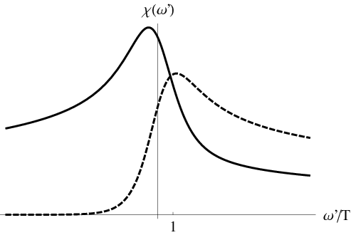
Using the results (7,8), we calculate spin susceptibility close to the $\Omega_{z^{\prime}}$ resonanse, with $\omega^{\prime}=\omega-\Omega_{z^{\prime}}$. We find $\chi_{T=0}\left(\omega^{\prime}\right)=\chi_{0}\Gamma\left(\lambda\right)\left(-\xi_{0}/\omega^{\prime}\right)^{\lambda},$ where $\chi_{0}=\frac{4N}{3\pi}J^{-1}.$ Note, that $\Im\chi_{l}=0$ below the threshold ($\omega^{\prime}<0)$ as it should be at $T=0$. These results can be easily generalized to the finite temperature $T\ll\mu$. As was shown in [14], finite-temperature correlation function in the FES problem can be obtained from the zero-temperature one by substitution $t\rightarrow\frac{\sinh\pi Tt}{\pi T}$. For the susceptibility, that gives:

This function is plotted in Fig. 3. The major effect of nonzero temperature is the appearence of absorption below threshold: $\chi\left(-\omega^{\prime}\gg T\right)\approx\chi_{T=0}\left(\omega^{\prime}\right)\left(1+i\sin\pi\lambda e^{-|\omega^{\prime}|/T}\right)$; in addition, the resonant peak appears to be smeared out: $\chi\left(|\omega^{\prime}|\ll T\right)\approx\chi_{0}e^{i\pi\lambda}\left(\frac{\xi_{0}}{2\pi T}\right)^{\lambda}$.

In conclusions, we have shown that certain (numerically, very weak) modification of the Yao-Kivelson version of Kitaev spin lattice leads to the ground-state of the Fermi-liquid type, with a Fermi energy $\mu\propto\sqrt{2}-J^{\prime}/J$. We have studied the model in the continuum limit of small Fermi-circle $\mu\ll J$ and at low temperatures $T\ll\mu$. Gapless excitations of the Fermi-sea do not carry spin themselves, but they determine the shape (9) of the resonance peak in the dynamic spin susceptibility.

We are grateful to A. Yu. Kitaev for numerous important discussions and advises. This research was supported by the RFBR grant # 10-02-00554 and by the RAS Program ”Quantum physics of condensed matter”.

References

- [1] P. W. Anderson, Mater. Res. Bull. 8, 153 (1973); P.Fazekas and P. W. Anderson, Philos.Mag. 30, 432 (1974).
- [2] P.W. Anderson, Science, 235, 1196 (1987).
- [3] X.-G. Wen, Phys. Rev., B 65, 165113 (2002)
- [4] C. Lhuillier, ”Frustrated Quantum Magnets”, arXiv:cond-mat/0502464v1 , lecture course, 2002.
- [5] G. Misguich, ”Quantum spin liquids”, arXiv:0809.2257 lecture course at the Les Houches School, 2008.
- [6] A. Yu. Kitaev, Ann. Phys. 321, 2 (2006)
- [7] G. Baskaran, S. Mandal and R. Shankar, Phys. Rev. Lett. 98, 247201 (2007).
- [8] D. N. Sheng, O. I. Motrunich, and M. P. A. Fisher Phys. Rev. B 79, 205112 (2009).
- [9] H. Yao and S. Kivelson, Phys. Rev. Lett. 99 , 247203 (2007)
- [10] H. Yao, S. Zhang and S. Kivelson, Phys. Rev. Lett. 102, 217202 (2008)
- [11] G. Baskaran, G.Santosh and R. Shankar, arXiv:0908.1614
- [12] S. B. Chung, H. Yao, T. L. Hughes, E. A. Kim, arXiv:0909.2655
- [13] P. Nozieres, C. T. De Dominicis, Phys. Rev. 178, 1097 (1969)
- [14] B. Braunecker, Phys. Rev. B 73, 075122 (2006)