Similarity-Based Classification in Partially Labeled Networks
Abstract
We propose a similarity-based method, using the similarity between nodes, to address the problem of classification in partially labeled networks. The basic assumption is that two nodes are more likely to be categorized into the same class if they are more similar. In this paper, we introduce ten similarity indices, including five local ones and five global ones. Empirical results on the co-purchase network of political books show that the similarity-based method can give high accurate classification even when the labeled nodes are sparse which is one of the difficulties in classification. Furthermore, we find that when the target network has many labeled nodes, the local indices can perform as good as those global indices do, while when the data is spares the global indices perform better. Besides, the similarity-based method can to some extent overcome the unconsistency problem which is another difficulty in classification.
Keywords:
complex networks , similarity , classification , labeled networkPACS
89.20.Ff , 89.75.Hc , 89.65.-s1 Introduction
Recently, the problem of within-network classification in partial labeled networks has attracted much attention. Given a network with partial nodes being labeled, the problem is to predict the labels of these unlabeled nodes based on the known labels and the network structure. Many algorithms have been proposed. These methods can be widely applied to many fileds, such as the hypertext categorization [1, 2], distinguishing the fraud and legit users in cell phone network [3], detecting whether an email is for a certain task [4] and predicting the disease-related genes [5]. Generally speaking, the known methods can be classified into two groups. One is collective classification, which refers to the combined classification by using three types of correlations: (1) between the node’s label and its attributes, (ii) between node’s label and its neighbor’s attributes, (iii) between node’s label and its neighbor’s label (see a brief introduction in Ref. [6]). One remarkably advantage of this method is its high ability to learn the dependency structure, such as positive or negative correlation (i.e. consistency or unconsistency). However, when the labeled nodes are sparse, this method is difficult to give accurate classification. The sparse problem can be solved by another group of methods, named semi-supervised learning, which make use of both labeled and unlabeled data for training (see Ref. [7] for more information). The latent assumption of this method is the consistency with the label information, namely the nearby nodes tend to have the same label. Therefore when this assumption does not hold the performance of this method will be largely degraded. Brian et al. proposed a method by adding ghost edges between every pair of labeled and unlabeled node to the target network, which enable the flow of information from the labeled nodes to the unlabeled nodes [3]. They assigned a weight to each ghost edge based on the score of the two endpoints obtained by the Even-step random walk with restart (Even-step RWR)algorithm. The experimental results on real-world data showed that their method can to some extent solve the sparse problem and negative correlation problem (i.e. unconsistency), and perform well while the existing approaches, such as collective classification and semi-supervised learning, will fail. In this paper, we compare the performances of Even-step RWR index with other nine similarity indices which have been widely used in link prediction problem [8, 9, 10]. These include five local indices, namely the Common Neighbors [11], Jaccard coefficient [12], Sørensen index [13], Adamic-Adar index [14] and Resource Allocation index [9], and four global indices, namely Katz index [15], Average Commute Time [16], cosine based on the Pseudoinverse of the Laplacian matrix () and Random walk With Restart (RWR) [17]. In addition, we also consider a simple relational neighbors algorithm, which claims that an unlabeled node tends to have the same label with its neighbors [18]. Empirical results on the co-purchase network of political books show that the similarity-based methods perform better than the relational neighbors algorithm. Especially when the labeled nodes are sparse, the improvement is prominent. Furthermore, when the data is dense, the local indices perform as good as the global indices, while when the data is spare the global indices will perform better.
The rest of this paper is organized as follows. In section 2 we introduce ten similarity indices, including five indices based on local information and others based on global information. Section 3 describes the metric to evaluate the algorithm’s accuracy. Section 4 shows the experimental results of the ten indices on the co-purchase network of political books. Finally, we conclude this paper in section 5.
2 Similarity indices
We consider five local similarity indices as well as five global ones. All are defined based on the network structure. A short introduction of each index is shown as:
(1) Common Neighbors — For a node , let denote the set of neighbors of . By common sense, two nodes, and , are more similar if they have many common neighbors. The simplest measure of this neighborhood overlap is the directed count, namely
| (1) |
where is the cardinality of the set . It is obvious that , where is the adjacency matrix, in which if and are directly connected and otherwise. Note that, is also the number of different paths with length 2 connecting and .
(2) Jaccard Index [12] — This index was proposed by Jaccard over a hundred years ago, and is defined as
| (2) |
(3) Sørensen Index [13] — This index is used mainly for ecological community data, and is defined as
| (3) |
(4) Adamic-Adar Index [14] — This index refines the simple counting of common neighbors by assigning the less-connected neighbors more weight, and is defined as:
| (4) |
(5) Resource Allocation [9]— Consider a pair of nodes, and , which are not directly connected. The node can send some resource to , with their common neighbors playing the role of transmitters. In the simplest case, we assume that each transmitter has a unit of resource, and will equally distribute it between all its neighbors. The similarity between and can be defined as the amount of resource received from , which is:
| (5) |
Clearly, this measure is symmetric, namely . Note that, although resulting from different motivations, the AA index and RA index have the very similar form. Indeed, they both depress the contribution of the high-degree common neighbors in different ways. AA index takes the form while RA index takes the linear form. The difference is insignificant when the degree, , is small, while it is great when is large. Therefor, RA index punishes the high-degree common neighbors heavily.
(6) Katz Index [15] — This measure is based on the ensemble of all paths, which directly sums over the collection of paths and exponentially damped by length to give the short paths more weights. The mathematical expression reads
| (6) |
where is the set of all paths with length connecting and , and is a free parameter controlling the weights of the paths. Obviously, a very small yields a measure close to CN, because the long paths contribute very little. The matrix can be written as . Note that, must be lower than the reciprocal of the maximum of the eigenvalues of matrix to ensure the convergence.
(7) Average Commute Time [16] — Denoting by the average number of steps required by a random walker starting form node to reach node , the average commute time between and is , which can be computed in terms of the Pseudoinverse of the Laplacian matrix , as:
| (7) |
where denotes the corresponding entry in . Assuming two nodes are considered to be more similar if they have a small average commute time, then the similarity between the nodes and can be defined as the reciprocal of , namely
| (8) |
(8) Cosine based on [16] — This index is an inner-product based measure, which is defined as the cosine of node vectors, namely
| (9) |
(9) Random walk with restart [17] — This index is a direct application of the PageRank algorithm. Consider a random walker starting from node , who will iteratively moves to a random neighbor with probability and return to node with probability . Denote by the probability this random walker locates at node in the steady state, then we have
| (10) |
where is an vector with the element equal to and others all equal to , and where . The solution is straightforward, as
| (11) |
Then we define the similarity between node and node equals .
(10) Even-step RWR [3] — To avoid the immediate neighbors, we can consider only the even-length paths. Mathematically, we should replace the transition matrix with .
For comparison, we compare the above-mentioned ten indices with the simplest method, says Relational Neighbors (RN) [18]. Given an unlabeled node , the probability that its label is equals
| (12) |
where is the set constituted by ’s neighbors whose label is , and is the set of ’s neighbors being labeled.
3 Method
Consider an unweighted undirected network of both labeled and unlabeled nodes: , where is the set of nodes, is the set of links and is the set of labels. For each pair of nodes, and , every algorithm referred in this paper assigns a score as . For an unlabeled node , the probability that it belongs to is
| (13) |
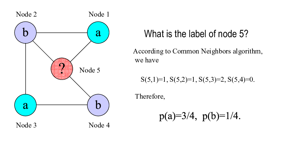
where . The predicted label of node is determined by the largest . If there are more than one maximum values, we randomly select one. A simple example is shown in Fig. 1, where there are two kinds of labels (i.e. and ) and five nodes, four of which are labeled already. Our task is to predict the label of the node 5. According to the common neighbors algorithm, we obtain the similarity between node 5 and the other four labeled nodes, and then we infer that the probability that node 5 is labeled by equals .
To test the algorithm’s accuracy, all the labeled nodes are randomly divided into two parts: the training set, , is treated as known information, while the probe set, , is used for testing. We denote the proportion of labeled nodes divided into training set, which is considered as the density index. A smaller indicates a sparser labeled network. The accuracy is quantified by the probability that we predict right. For a testing node whose label is , if , we predict right, and thus . If there is maximum values corresponding to different labels and the right label is one of them, we have . Run over all the testing nodes we have the accuracy equals
| (14) |
where is the number of nodes in the probe set. For example, if there are two categories in the target network, namely and , accuracy can be obtained by
| (15) |
where is the number of nodes in probe set being predicted right and is the number of nodes having the same probability of two labels (i.e. ).
4 Empirical results
We compare the above-mentioned ten similarity indices on the co-purchases network of political books [19]. This network contains 105 nodes (books) and 441 edges. All books are classified into three categories, neutral, liberal and conservative. For simplicity, we start the experiments with the sampled networks containing only two classes. Therefore, we sample three labeled networks with three tasks as follows:
Task 1: Whether an unlabel node is neutral? For this task, we label the books which are neutral by and others by (i.e. not neutral).
Task 2: Whether an unlabel node is liberal? For this task, we label the books which are liberal by and others by (i.e. not liberal).
Task 3: Whether an unlabel node is conservative? We label the books which are conservative by and others by (i.e. not conservative).
Table.1 summarize the basic statistics of these three sampled networks corresponding to task 1, task 2 and task 3 respectively. () is the number of nodes labeled by . indicates the number of edges connecting to the nodes labeled by . Denote by the number of edges whose two endpoints have the same label , then indicats the local consistency of the subgraph constituted by the nodes labeled by and the edges connecting to these nodes. is the local consistency of the whole network, which reads , where is the total number of edges of the whole network (here ). Note that, . Here, we further develop the definition of local consistency to two-step consistency denoting by which equals to the number of path with length 2 whose two endpoints have the same label divide by the number of the path with length 2. Clearly, the common neighbor index will perform well in the network with high . Four simple examples of calculating , and are shown in Fig. 2. One can see that in the first graph, because of , RN will perform very bad, while CN performs very good (). However in the forth graph both RN and CN can give good performance.


| Net | ||||||||||
|---|---|---|---|---|---|---|---|---|---|---|
| Net1 | 13 | 92 | 67 | 432 | 9 | 374 | 0.134 | 0.866 | 0.869 | 0.864 |
| Net2 | 43 | 62 | 208 | 269 | 172 | 233 | 0.827 | 0.866 | 0.918 | 0.894 |
| Net3 | 49 | 56 | 236 | 251 | 190 | 205 | 0.805 | 0.817 | 0.890 | 0.882 |
Comparison of the ten similarity indices on three sampled networks are shown in Fig. 3. The subgraphs (a), (c) and (e) show the results of the local indices, while (b), (d) and (f) report the results of the global indices. It is interesting that all these five local indices give almost the same results especially when the density of labeled nodes is small. This is because all these five indices are common-neighbor based and when is small whether an unlabeled node relevant with a labeled node play a more important role than the exact correlation (similarity score) between them. Furthermore, because of the high of these three networks, all the common-neighbor-based indices performs well and even when the data is sparse they can give much better prediction than RN. Compare with global indices, the local indices can give competitively accurate classification when is large, but when the labeled data is sparse, for most unlabeled node it is too difficult to find a labeled node nearby, and thus the global indices will perform better. Among these five global indices, the performance of Katz index, RWR and even-step RWR are stable, while the performance of ACT and are not. For example, in sampled network 1, the ACT index performs very well but is even worse than pure chance. However, in sampled network 3, the index preforms the best but the ACT index performs even worse than the simplest method RN.
Obviously, it will be more difficult to obtain highly accurate classification when we consider many categories together. We futher carry out an experiment on the network containing all the three categories. Our task is to detect the category of an unlabel book, namely is it neutral, liberal or conservative? We label the books by (i.e. neutral), (i.e. liberal) and (i.e. conservative) according to their categories. The local consistency and two-step consistency of this network are 0.8413 and 0.8204 respectively, which are all lower than the three sampled networks containing only two classes, and thus the accuracy is also lower, as shown in Fig. 4. One can see that the results are similar to the one on the sampled network 3 where the biggest class, conservative, is considered. This result demonstrates that the majorities play the main role.


5 Conclusion and Discussion
In this paper, we investigated the similarity-based classification for partial labeled network. The basic assumption is that two nodes are more likely to have the same label if they are more similar to each other. We introduced ten similarity indices which have been widely used to solve the link prediction problem of complex networks, including five common-neighbor-based indices, namely Common Neighbors, Jaccard coefficient, Sørensen index, Adamic-Adar index and Resource Allocation index, and five global indices, namely Katz index, Average Commute Time, cosine based on the Pseudoinverse of the Laplacian matrix (), Random walk With Restart (RWR) and Even-step RWR. We carried out the experiments on the co-purchase network of political books. The results showed that the similarity-based classification perform much better than the relational neighbors algorithm, especially when the labeled nodes are sparse. Furthermore, we found that when the data is dense the local indices can perform as good as the global indices. However, when the data is sparse, for an unlabeled node it is too difficult to find a labeled node nearby, and thus the global indices perform better. Compare with the former proposed algorithms the group of similarity-based classification methods has three advantages: firstly, it can to some extent solve the sparse data problem by using the global indices; secondly, when the network consistency assumption is not hold it can still give high accurate classification; thirdly, without any learning process this method has lower calculation complexity than other complicated methods.
However, there are still some open problems left. For example what is the relation between the network label structure and the performance of each similarity index. In-depth analysis on the modeled networks may be helpful, where we can control the label density, network consistency and also the proportion of each class. Anyway, we hope this work can provide a novel view for the study of classification in partial labeled networks and we believe that there is still a large space for further contribution. For example, when the number of nodes in one class is much lager than in the others, the unlabeled nodes are more likely to have the same labels with the majority. To solve this problem we can only consider the top- similar labeled nodes when calculate the probability. In addition, we can also use negative correlation in the adjacent matrix directly, namely for the nonzero element in if the node and have the different labels, we set . To do this, we can not only obtain the strength of the correlation between the unlabeled node and the labeled one but also know the correlation type, positive or negative.
6 ACKNOWLEDGEMENT
We acknowledge Tao Zhou for his assistance of manuscript preparation. This work is partially supported by the Swiss National Science Foundation (200020-121848), the China Postdoctoral Science Foundation (20080431273) and the National Natural Science Foundation of China (60973069, 90924011).
References
- [1] S. Chakrabarti, B. E. Dom, P. Indyk, Enhanced hypertext categorization using hyperlinks, in Proceedings of SIGMOD-98, ACM International Conference on Management of Data (ACM Press, Seattle, WA, 1998).
- [2] Y. Yang, S. Slattery, R. Ghani, A Study of Approaches to Hypertext Categorization, Journal of Intelligent Information Systems 18, 219 (2002).
- [3] B. Gallagher, H. Tong, T. Eliassi-Rad, C. Faloutsos, Using ghost edges for classification in sparsely labeled networks, in Proceedings of the ACM SIGKDD International Conference on Knowledge Discovery and Data Mining (ACM Press, New York, 2008).
- [4] V. R. Carvalho, W. W. Cohen, On The Collective Classification of Email ”Speech Acts”, in Proceedings of the 28th annual international ACM SIGIR conference on Research and development in information retrieval (ACM Press, New York, 2005).
- [5] L. Zhang, K. Hu, Y. Tang, Predicting disease-related genes by topological similarity in human protein-protein interaction network, Cent. Eur. J. Phys., DOI:10.2478/s11534-009-0114-9, (2009).
- [6] P. Sen, G. Namata, M. Bilgic, L. Getoor, B. Gallagher, T. Eliassi-Rad, Collective classification in network data, AI Magazine 29, 93 (2008).
- [7] X. Zhu, A. B. Goldberg, Synthesis Lectures on Artificial Intelligence and Machine Learning 3, 1 (2009).
- [8] D. Liben-Nowell, J. Kleinberg, The Link-prediction problem for social networks, J. Am. Soc. Inf. Sci. &. Technol. 58, 1019 (2007).
- [9] T. Zhou, L. Lü, Y.-C. Zhang, Predicting missing links via local information, Eur. Phys. J. B 71, 623 (2009).
- [10] L. Lü, C.-H. Jin, T. Zhou, Effective and efficient similarity index for link prediction of complex networks, Phys. Rev. E 80, 046122 (2009).
- [11] F. Lorrain, H. C. White, Structural equivalence of individual in social networks, J. Math. Sociol. 1, 49 (1971).
- [12] P. Jaccard, Etude comparative de la distribution florale dans une portion des Alpes et des Jura, Bull. Soc. Vaud. Sci. Nat. 37, 547 (1901).
- [13] T. Sørensen, A method for establishing groups of equal magnitude in plant sociology based on similarity of species contentand and its application to analyses of the vegetation on Danish commons, Biol. Skr. 5, 1 (1948).
- [14] L. A. Adamic, E. Adar, Friends and neighbors on the Web, Social Networks 25, 211 (2003).
- [15] L. Katz, A new status index derived from sociometric analysis, Psychmetrika 18, 39 (1953).
- [16] D. J. Klein, M. Randic, Resistance distance, J. Math. Chem. 12, 81 (1993).
- [17] S. Brin, L. Page, The anatomy of a large-scale hypertextual Web search engine, Computer Networks and ISDN Systems 30, 107 (1998).
- [18] S. Macskassy, F. Provost, A simple relational classifier, in Proceedings of the 2nd International Workshop on Multi-Relational Data Mining (ACM Press, New York, 2003).
- [19] V. Krebs, Working in the Connected World: Book Network, International Association for Human Resource Information Management Journal 4, 87 (2000).