Pseudo-Anosovs on closed surfaces having small entropy and the Whitehead sister link exterior

Eiko Kin Note: The author is partially supported by Grant-in-Aid for Young Scientists (B) (No. 20740031), MEXT, Japan. Last compile 08/15/2011. 2010 Mathematics Subject Classification: Primary 57M27, 37E30, Secondary 37B40. Key words and phrases: mapping class group, pseudo-Anosov, dilatation, entropy, fibered $3$-manifold. and Mitsuhiko Takasawa

Abstract

We denote by $\delta_{g}$ (resp. $\delta_{g}^{+}$ ), the minimal dilatation for pseudo-Anosovs (resp. pseudo-Anosovs with orientable invariant foliations) on a closed surface of genus $g$ . This paper concerns the pseudo-Anosovs which occur as monodromies of fibrations on manifolds obtained from the Whitehead sister link exterior $W$ by Dehn filling two cusps, where the fillings are on the boundary slopes of fibers of $W$ . We give upper bounds of $\delta_{g}$ for $g\equiv 0,1,5,6,7,9\pmod{10}$ , $\delta_{g}^{+}$ for $g\equiv 1,5,7,9\pmod{10}$ . Our bounds improve the previous one given by Hironaka. We note that the monodromies of fibrations on $W$ were also studied by Aaber and Dunfield independently.

1 Introduction

Let $\mathrm{Mod}(\varSigma)$ be the mapping class group on an orientable surface $\varSigma$ . An element $\phi\in\mathrm{Mod}(\varSigma)$ which contains a pseudo-Anosov homeomorphism $\Phi:\varSigma\rightarrow\varSigma$ as a representative is called a pseudo-Anosov mapping class. There are two numerical invariants for pseudo-Anosov mapping classes. One is the dilatation $\lambda(\phi)>1$ (or the entropy $\mathrm{ent}(\phi)=\log\lambda(\phi)$ ) which is defined to be the dilatation $\lambda(\Phi)$ of $\Phi$ , and the other is the hyperbolic volume $\mathrm{vol}(\phi)=\mathrm{vol}({\mathbb{T}}(\phi))$ of the mapping torus ${\mathbb{T}}(\Phi)$ . It is natural to ask whether there is a relation between $\mathrm{ent}(\phi)$ and $\mathrm{vol}(\phi)$ . Computer experiments in [13] tell us that if we fix a surface $\varSigma$ , then pseudo-Anosovs with small dilatation have small volume. This is true in a sense. In fact it is proved in [6] that pseudo-Anosovs on any surfaces with small dilatation have the bounded volume, see Theorem 1.4.

We denote by $\delta_{g}$ , the minimal dilatation for pseudo-Anosov elements $\phi\in\mathrm{Mod}(\varSigma_{g})$ on a closed surface $\varSigma_{g}$ of genus $g$ . A natural question is: what is the value $\delta_{g}$ ? To discuss the minimal dilatations, we introduce the polynomial

f_{(k,\ell)}(t)=t^{2k}-t^{k+\ell}-t^{k}-t^{k-\ell}+1\hskip 5.69054pt\mbox{for}\ k>0,\ -k<\ell<k.

This polynomial has the largest real root $\lambda_{(k,\ell)}$ which is greater than $1$ (Theorem 3.2 and Lemma 4.4). For any fixed $\ell>0$ , it follows that $k\log\lambda_{(k,\ell)}$ converges to $\log(\tfrac{3+\sqrt{5}}{2})$ if $k$ goes to $\infty$ (Lemma 4.16). It is easy to show that $\delta_{1}=\lambda_{(1,0)}=\tfrac{3+\sqrt{5}}{2}$ . It was proved by Cho-Ham that $\delta_{2}=\lambda_{(2,1)}\approx 1.72208$ [4]. It is open to determine the values $\delta_{g}$ for $g\geq 3$ . Questions on properties of $\delta_{g}$ were posed by McMullen and Farb:

Question 1.1 ([23] for (1), [5] for (2)).

(1): Does $\displaystyle\lim_{g\to\infty}g\log\delta_{g}$ exist? What is its value?
(2): Is the sequence $\{\delta_{g}\}_{g\geq 2}$ (strictly) monotone decreasing?

Related questions are ones for orientable pseudo-Anosovs. A pseudo-Anosov mapping class $\phi$ is said to be orientable if the invariant (un)stable foliation of a pseudo-Anosov homeomorphism $\Phi\in\phi$ is orientable. We denote by $\delta_{g}^{+}$ , the minimal dilatation for orientable pseudo-Anosov elements of $\mathrm{Mod}(\varSigma_{g})$ . The minima $\delta_{g}^{+}$ were determined for $g=2$ by Zhirov [31], for $3\leq g\leq 5$ by Lanneau-Thiffeault [17], and for $g=8$ by Lanneau-Thiffeault and Hironaka [17, 9]. Those values are given by $\delta_{2}^{+}=\lambda_{(2,1)}$ , $\delta_{3}^{+}=\lambda_{(3,1)}=\lambda_{(4,3)}\thickapprox 1.40127$ , $\delta_{4}^{+}=\lambda_{(4,1)}\thickapprox 1.28064$ , $\delta_{5}^{+}=\lambda_{(6,1)}=\lambda_{(7,4)}\thickapprox 1.17628$ and $\delta_{8}^{+}=\lambda_{(8,1)}\thickapprox 1.12876$ .

Lanneau-Thiffeault obtained the inequality $\delta_{5}^{+}\leq\delta_{6}^{+}$ ([17]) which implies that $\{\delta^{+}_{g}\}_{g\geq 2}$ is not strictly monotone decreasing. This leads us to ask an alternative question related to Question 1.1(2): is the sequence $\{\delta_{g}^{+}\}_{g\geq 2}$ monotone decreasing? Also, one can ask: which $g$ does the inequality $\delta_{g}<\delta^{+}_{g}$ hold? It is easy to see that $\delta_{1}=\delta_{1}^{+}$ . The equality $\delta_{g}=\delta_{g}^{+}$ holds for $g=2$ [4, 31]. We do not know whether $\delta_{3}=\delta_{3}^{+}$ holds or not. By work of Lanneau-Thiffeault and Hironaka, it follows that $\delta_{g}<\delta_{g}^{+}$ for $g=4,6,8$ [17, 9].

To discuss Question 1.1(1), we recall the previous upper bound of $\delta_{g}$ given by Hironaka.

Theorem 1.2 ([9]).

(1): $\delta_{g}\leq\lambda_{(g+1,3)}$ if $g\equiv 0,1,3,4\pmod{6}$ and $g\geq 3$ .
(2): $\delta_{g}\leq\lambda_{(g+1,1)}$ if $g\equiv 2,5\pmod{6}$ and $g\geq 5$ .

By using Lemma 4.16 and Theorem 1.2, the following asymptotic inequality holds.

Theorem 1.3 ([9]).

$\displaystyle\lim_{g\to\infty}\sup g\log\delta_{g}\leq\log(\tfrac{3+\sqrt{5}}{2})$ .

This improves the upper bound $g\log\delta_{g}\leq g\log\delta^{+}_{g}\leq\log(2+\sqrt{3})$ for each $g\geq 2$ by Minakawa [22] and Hironaka-Kin [10]. Since $\log\delta_{g}$ tends to $0$ as $g$ tends to $\infty$ , Theorem 1.3 implies that

\lim_{g\to\infty}\sup|\chi(\varSigma_{g})|\log\delta_{g}\leq 2\log(\tfrac{3+\sqrt{5}}{2}),

where $\chi(\varSigma)$ is the Euler characteristic of a surface $\varSigma$ .

Let $N$ be the magic manifold which is the exterior of the $3$ chain link $\mathcal{C}_{3}$ illustrated in Figure 1(left). This manifold has the smallest known volume among orientable hyperbolic $3$ -manifolds having $3$ cusps. Many manifolds having at most $2$ cusps with small volume are obtained from $N$ by Dehn fillings, see [20]. In this paper, we study the small dilatation pseudo-Anosov homeomorphisms which occur as monodromies of fibrations on manifolds obtained from $N$ by Dehn filling all three cusps. In [6], Farb, Leininger and Margalit introduced small dilatation pseudo-Anosov homeomorphisms which we recall below.

Refer to caption — Figure 1: (left) $3$ chain link $\mathcal{C}_{3}$ . (center) $(-2,3,8)$ -pretzel link or Whitehead sister link. (right) link $6_{2}^{2}$ .

For any number $P>1$ , define the set of pseudo-Anosov homeomorphisms

\Psi_{P}=\{\mbox{pseudo-Anosov\ }\Phi:\varSigma\rightarrow\varSigma\ |\ \chi(\varSigma)<0,\ |\chi(\varSigma)|\log\lambda(\Phi)\leq\log P\}.

They call elements $\Phi\in\Psi_{P}$ small dilatation pseudo-Anosov homeomorphisms. Theorem 1.3 says that if one takes $P$ sufficiently large, then $\Psi_{P}$ contains a pseudo-Anosov homeomorphism $\Phi_{g}:\varSigma_{g}\rightarrow\varSigma_{g}$ for each $g\geq 2$ . By a result by Hironaka-Kin [10], $\Psi_{P}$ also contains a pseudo-Anosov homeomorphism $\Phi_{n}:D_{n}\rightarrow D_{n}$ on an $n$ -punctured disk $D_{n}$ for each $n\geq 3$ . Let $\varSigma^{\circ}\subset\varSigma$ be the surface obtained by removing the singularities of the (un)stable foliation for $\Phi$ and $\Phi|_{\varSigma^{\circ}}:\varSigma^{\circ}\rightarrow\varSigma^{\circ}$ denotes the restriction. Observe that $\lambda(\Phi)=\lambda(\Phi|_{\varSigma^{\circ}})$ . The set

\Psi_{P}^{\circ}=\{\Phi|_{\varSigma^{\circ}}:\varSigma^{\circ}\rightarrow\varSigma^{\circ}\ |\ (\Phi:\varSigma\rightarrow\varSigma)\in\Psi_{P}\}

is infinite. Let $\mathcal{T}(\Psi_{P}^{\circ})$ be the set of homeomorphism classes of mapping tori by elements of $\Psi_{P}^{\circ}$ .

Theorem 1.4 ([6]).

The set $\mathcal{T}(\Psi_{P}^{\circ})$ is finite. Namely, for each $P>1$ , there exist finite many complete, non compact hyperbolic $3$ -manifolds $M_{1},M_{2},\cdots,M_{r}$ fibering over $S^{1}$ so that the following holds. Any pseudo-Anosov $\Phi\in\Psi_{P}$ occurs as the monodromy of a Dehn filling of one of the $M_{k}$ . In particular, there exists a constant $V=V(P)$ such that $\mathrm{vol}(\Phi)\leq V$ holds for any $\Phi\in\Psi_{P}$ .

Agol also proved Theorem 1.4 by using periodic splitting sequences of pseudo-Anosov mapping tori [3]. By Theorem 1.4, one sees that the following sets $\mathcal{U}$ , $\mathcal{U}^{+}$ and $\mathcal{V}$ are finite.

		$\displaystyle\mathcal{U}$	$\displaystyle=\{{\mathbb{T}}(\Phi\|_{\varSigma^{\circ}})\ \|\ g\geq 2,\ \Phi\ \mbox{is\ a\ pseudo-Anosov\ homeomorphism\ on\ }\varSigma=\varSigma_{g}\mbox{\ such\ that\ }\lambda(\Phi)=\delta_{g}\},$
		$\displaystyle\mathcal{U}^{+}$	$\displaystyle=\{{\mathbb{T}}(\Phi\|_{\varSigma^{\circ}})\ \|\ g\geq 2,\ \Phi\ \mbox{is\ an\ orientable\ pseudo-Anosov\ homeomorphism}$
			$\displaystyle\hskip 56.9055pt\mbox{on\ }\varSigma=\varSigma_{g}\mbox{\ such\ that\ }\lambda(\Phi)=\delta_{g}^{+}\},$
		$\displaystyle\mathcal{V}$	$\displaystyle=\{{\mathbb{T}}(\Phi\|_{\varSigma^{\circ}})\ \|\ n\geq 3,\ \Phi\ \mbox{is\ a\ pseudo-Anosov\ homeomorphism\ on\ }\varSigma=D_{n}\mbox{\ such\ that\ }\lambda(\Phi)=\delta(D_{n})\},$

where $\delta(D_{n})$ denotes the minimal dilatation for pseudo-Anosov elements of $\mathrm{Mod}(D_{n})$ on an $n$ -punctured disk $D_{n}$ .

The previous study [15] by the authors implies that $N\in\mathcal{V}$ . In fact, the mapping class $\phi\in\mathrm{Mod}(D_{4})$ represented by the $4$ -braid $\sigma_{1}\sigma_{2}\sigma_{3}^{-1}$ has the minimal dilatation $\delta(D_{4})$ [16]. For the pseudo-Anosov representative $\Phi$ of this mapping class $\phi$ , the mapping torus ${\mathbb{T}}(\Phi|_{\varSigma^{\circ}})$ is homeomorphic to $N$ [15]. Moreover for each $n\geq 6$ (resp. $n=3,4,5$ ), a pseudo-Anosov homeomorphism $\Phi_{n}:D_{n}\rightarrow D_{n}$ having the smallest known dilatation (resp. smallest dilatation) occurs as the monodromy on a particular fibration on a manifold obtained from $N$ by Dehn filling [15]. See also work of Venzke [29].

Hironaka obtained Theorems 1.2 and 1.3 by viewing the monodromies of fibrations on manifolds obtained from the $6_{2}^{2}$ link exterior $S^{3}\setminus 6_{2}^{2}$ by Dehn filling two cusps. (For the link $6_{2}^{2}$ , see Figure 1(right) or Rolfsen’s table [24, Appendix C].) There exists an orientable monodromy $:\varSigma_{2}\rightarrow\varSigma_{2}$ with dilatation $\delta_{2}=\delta_{2}^{+}$ of a fibration on a manifold obtained from $S^{3}\setminus 6_{2}^{2}$ by Dehn filling two cusps. This implies that $S^{3}\setminus 6_{2}^{2}\in\mathcal{U}\cap\mathcal{U}^{+}$ (Lemma 4.24 or [9]). We see that $S^{3}\setminus 6_{2}^{2}$ is homeomorphic to $N(\tfrac{-1}{2})$ (see [20, Table A.1] for example), where $N(r)$ is the manifold obtained from $N$ by Dehn filling one cusp along the slope $r$ . As mentioned, computer experiments say that the pseudo-Anosovs having small dilatation have small volume, and $N$ is the candidate having the smallest volume among orientable $3$ -manifolds with $3$ cusps. These results led us to see monodromies of fibrations on manifold obtained from $N$ by Dehn filling.

In this paper, we investigate the fibrations on manifolds obtained from the three $2$ -cusped manifolds $N(\tfrac{-1}{2})$ , $N(\tfrac{-3}{2})$ and $N(2)$ by Dehn filling $2$ cusps. The second one $N(\tfrac{-3}{2})$ is homeomorphic to $N(-4)$ and this is the Whitehead sister link exterior, i.e, the $(-2,3,8)$ -pretzel link exterior (see [20, Table A.1]), see Figure 1(center). The manifold $N(\tfrac{-3}{2})$ and the Whitehead link exterior have the smallest volume among orientable $2$ -cusped hyperbolic $3$ -manifolds [2]. We shall see that $N(\tfrac{-3}{2})$ and $N(2)$ are elements of $\mathcal{U}^{+}$ (Lemmas 4.21, 4.36). Our main result is that $N(\tfrac{-3}{2})$ (resp. $N(2)$ ) also admits Dehn fillings giving a sequence of fibers over the circle, with closed fibers $\varSigma_{g}$ of genus $g$ for each $g\geq 3$ such that the monodromies associated to the fibrations satisfy the same asymptotic inequality as Theorem 1.3. More precisely, we shall prove the following.

Theorem 1.5.

Let $r\in\{\tfrac{3}{-2},\tfrac{1}{-2},2\}$ . For each $g\geq 3$ , there exist $\varSigma_{g}$ -bundles over the circle obtained from $N(r)$ by Dehn filling all two cusps along the boundary slopes of fibers of $N(r)$ . Among them, there exist the monodromies $\Phi_{g}(r):\varSigma_{g}\rightarrow\varSigma_{g}$ of the fibrations such that

(1): $\displaystyle\lim_{g\to\infty}g\log\lambda(\Phi_{g})=\log(\tfrac{3+\sqrt{5}}{2})$ ,
(2): $\displaystyle\lim_{g\to\infty}\mathrm{vol}(\Phi_{g})=\mathrm{vol}(N(r))$ .

Independently, Aaber and Dunfield have investigated $\varSigma_{g}$ -bundles over the circle obtained from $N(\tfrac{-3}{2})$ by Dehn filling two cusps, see [1] and Remark 4.33. They have obtained similar results on the dilatation to those given in this paper. Theorem 1.5 in the case $r=\tfrac{-3}{2}$ was also established by [1].

By using monodromies on closed fibers coming from $N(\tfrac{-3}{2})$ , we find an upper bound of $\delta_{g}$ .

Theorem 1.6.

(1): $\delta_{g}\leq\lambda_{(g+2,1)}$ if $g\equiv 0,1,5,6\pmod{10}$ and $g\geq 5$ .
(2): $\delta_{g}\leq\lambda_{(g+2,2)}$ if $g\equiv 7,9\pmod{10}$ and $g\geq 7$ .

Theorem 1.7.

Let $g\equiv 2,4\pmod{10}$ . Suppose that $g+2\not\equiv 0$ $\pmod{4641(=3\cdot 7\cdot 13\cdot 17)}$ .

(1): $\delta_{g}\leq\lambda_{(g+2,3)}$ if $\gcd(g+2,3)=1$ .
(2): $\delta_{g}\leq\lambda_{(g+2,7)}$ if $3$ divides $g+2$ and $\gcd(g+2,7)=1$ .
(3): $\delta_{g}\leq\lambda_{(g+2,13)}$ if $21(=3\cdot 7)$ divides $g+2$ and $\gcd(g+2,13)=1$ .
(4): $\delta_{g}\leq\lambda_{(g+2,17)}$ if $273(=3\cdot 7\cdot 13)$ divides $g+2$ and $\gcd(g+2,17)=1$ .

We will verify the bounds in Theorems 1.6, 1.7 are sharper than the ones in Theorem 1.2 (see Propositions 4.26(1),(2) and 4.28). Theorems 1.6, 1.7 do not include the case $g\equiv 3,8\pmod{10}$ . This is because in this case, $N(\tfrac{-3}{2})$ can not give rise to the monodromy on a closed fiber of genus $g$ whose dilatation is strictly smaller than the one obtained from $N(\tfrac{-1}{2})$ , see Proposition 4.26(3),(4). However in case $g=8,13$ , we find a sharper upper bound than the one in Theorem 1.2. Let $\lambda_{(x,y,z)}$ be the largest real root of the polynomial

f_{(x,y,z)}(t)=t^{x+y-z}-t^{x}-t^{y}-t^{x-z}-t^{y-z}+1.

Proposition 1.8.

(1): $\delta_{8}\leq\lambda_{(18,17,7)}(\thickapprox 1.10403)<\lambda_{(9,1)}(\thickapprox 1.11350)$ .
(2): $\delta_{13}\leq\lambda_{(27,21,8)}(\thickapprox 1.07169)<\lambda_{(14,3)}(\thickapprox 1.07266)$ .

We turn to the study on $\delta_{g}^{+}$ . We record results by Lanneau-Thiffeault.

Theorem 1.9 ([17]).

The minimal dilatation $\delta_{g}^{+}$ for $g=6,7$ is not less than the largest real root of the following polynomial.

(1): $f_{(6,1)}(t)=t^{12}-t^{7}-t^{6}-t^{5}+1$ if $g=6$ . $(\delta_{6}^{+}\geq\lambda_{(6,1)}\thickapprox 1.17628.)$
(2): $f_{(9,2)}(t)=(t^{4}-t^{3}+t^{2}-t+1)(t^{14}+t^{13}-t^{9}-t^{8}-t^{7}-t^{6}-t^{5}+t+1)$ if $g=7$ . $(\delta_{7}^{+}\geq\lambda_{(9,2)}\thickapprox 1.11548.)$

Lanneau-Thiffeault asked the following.

Question 1.10 ([17]).

For $g$ even, is $\delta_{g}^{+}$ equal to the largest real root of the polynomial

f_{(g,1)}(t)=t^{2g}-t^{g+1}-t^{g}-t^{g-1}+1?

Namely, is $\delta_{g}^{+}$ equal to $\lambda_{(g,1)}$ for $g$ even?

An upper bound of $\delta_{g}^{+}$ given by Hironaka is as follows.

Theorem 1.11 ([9]).

(1): $\delta_{g}^{+}\leq\lambda_{(g+1,3)}$ if $g\equiv 1,3\pmod{6}$ .
(2): $\delta_{g}^{+}\leq\lambda_{(g,1)}$ if $g\equiv 2,4\pmod{6}$ .
(3): $\delta_{g}^{+}\leq\lambda_{(g+1,1)}$ if $g\equiv 5\pmod{6}$ .

We do not know whether there exists an orientable pseudo-Anosov homeomorphism of genus $g$ having the dilatation $\lambda_{(g,1)}$ (appeared in Question 1.10) or not for each $g\equiv 0\pmod{6}$ . Under the assumption that Question 1.10 is true, the inequality $\delta_{g}^{+}\leq\delta_{g+1}^{+}$ holds whenever $g\equiv 5\pmod{6}$ and $\delta_{g}<\delta_{g}^{+}$ holds for all even $g$ , see [9].

We give an upper bound of $\delta_{g}^{+}$ in the case $g\equiv 1,5,7,9\pmod{10}$ using orientable pseudo-Anosov monodromies coming from $N(\tfrac{-3}{2})$ .

Theorem 1.12.

(1): $\delta_{g}^{+}\leq\lambda_{(g+2,2)}$ if $g\equiv 7,9\pmod{10}$ and $g\geq 7$ .
(2): $\delta_{g}^{+}\leq\lambda_{(g+2,4)}$ if $g\equiv 1,5\pmod{10}$ and $g\geq 5$ .

We shall see that the bound in Theorem 1.12 improves the one in Theorem 1.11 (see Proposition 4.34). Theorem 1.12(1) together with Theorem 1.9(2) gives:

Corollary 1.13.

$\delta_{7}^{+}=\lambda_{(9,2)}$ .

Independently, Corollary 1.13 was established by Aaber and Dunfiled [1].

The following tells us that the sequence $\{\delta_{g}^{+}\}_{g\geq 2}$ is not monotone decreasing.

Proposition 1.14.

If Question 1.10 is true, then $\delta_{g}^{+}<\delta_{g+1}^{+}$ whenever $g\equiv 1,5,7,9\pmod{10}$ and $g\geq 7$ . In particular the inequality $\delta_{7}^{+}<\delta_{8}^{+}$ holds.

Our pseudo-Anosov homeomorphisms providing the upper bound of $\delta_{g}$ in Theorem 1.6(1) are not orientable (Remark 4.27). This together with the inequality $\lambda_{(7,1)}<\lambda_{(6,1)}=\delta_{5}^{+}$ implies:

Corollary 1.15.

$\delta_{5}<\delta_{5}^{+}$ .

We have a question:

Question 1.16.

Does the magic manifold $N$ satisfy the following (1),(2) and (3)?

(1): There exist Dehn fillings of $N$ giving an infinite sequence of fiberings over the circle, with closed fibers $\varSigma_{g_{i}}$ of genus $g_{i}\geq 2$ with $g_{i}\to\infty$ , and with monodromy $\Phi_{i}$ so that $\delta_{g_{i}}=\lambda(\Phi_{i})$ .
(2): There exist Dehn fillings of $N$ giving an infinite sequence of fiberings over the circle, with closed fibers $\varSigma_{g_{i}}$ of genus $g_{i}\geq 2$ with $g_{i}\to\infty$ , and with monodromy $\Phi_{i}$ having the orientable (un)stable foliation so that $\delta_{g_{i}}^{+}=\lambda(\Phi_{i})$ .
(3): There exist Dehn fillings of $N$ giving an infinite sequence of fiberings over the circle, with fibers $D_{n_{i}}$ having $n_{i}$ punctures with $n_{i}\to\infty$ , and with monodromy $\Phi_{i}$ so that $\delta(D_{n_{i}})=\lambda(\Phi_{i})$ .

The existence of the manifold satisfying each of (1),(2) and (3) is guaranteed from Theorem 1.4. Question 1.16 asks whether $N$ enjoys all (1),(2) and (3) or not.

The paper is organized as follows. We review basic facts in Section 2. The fibered faces and the entropy function for $N$ are described in Section 3. The (un)stable foliation for the monodromy of the fibration on $N$ is discussed in the section. We prove theorems in Section 4.

2 Notation and basic facts

2.1 Pseudo-Anosov

The mapping class group $\mathrm{Mod}(\varSigma)$ is the group of isotopy classes of orientation preserving homeomorphisms of an orientable surface $\varSigma$ , where the group operation is induced by composition of homeomorphisms. An element of this group is called a mapping class.

A homeomorphism $\Phi:\varSigma\rightarrow\varSigma$ is pseudo-Anosov if there exists a constant $\lambda=\lambda(\Phi)>1$ called the dilatation of $\Phi$ and there exists a pair of transverse measured foliations $\mathcal{F}^{s}$ and $\mathcal{F}^{u}$ such that

\Phi(\mathcal{F}^{s})=\tfrac{1}{\lambda}\mathcal{F}^{s}\ \mbox{and}\ \Phi(\mathcal{F}^{u})=\lambda\mathcal{F}^{u}.

Measured foliations $\mathcal{F}^{s}$ and $\mathcal{F}^{u}$ are called the stable and unstable foliations or invariant foliations for $\Phi$ . In this case the mapping class $\phi=[\Phi]$ is called pseudo-Anosov. We define the dilatation of $\phi$ , denoted by $\lambda(\phi)$ , to be the dilatation of $\Phi$ .

The (topological) entropy $\mathrm{ent}(f)$ is a measure of the complexity of a continuous self-map $f$ on a compact manifold, see for instance [30]. The inequality

\log\mathrm{sp}(f_{*})\leq\mathrm{ent}(f)

holds (see [19]), where $\mathrm{sp}(f_{*})$ is the spectral radius of the induced map $f_{*}:H_{1}(S;{\mathbb{R}})\rightarrow H_{1}(S;{\mathbb{R}})$ on the first homology group. For any pseudo-Anosov homeomorphism $\Phi:\varSigma\rightarrow\varSigma$ , the equality

\mathrm{ent}(\Phi)=\log(\lambda(\Phi))

holds and $\mathrm{ent}(\Phi)$ attains the minimal entropy among all homeomorphisms which are isotopic to $\Phi$ , see [7, Exposé 10]. We denote by $\mathrm{ent}(\phi)$ , this characteristic number. If $\Phi$ has orientable invariant foliations, then the equality

\log\mathrm{sp}(\Phi_{*})=\mathrm{ent}(\Phi)

holds, see [25]. The converse is true:

Theorem 2.1 ([17]).

A pseudo-Anosov homeomorphism $\Phi$ is orientable if and only if $\mathrm{sp}(\Phi_{*})=\lambda(\Phi)$ .

If we fix a surface $\varSigma$ and take a constant $c>1$ , then the set of dilatations $\lambda(\Phi)<c$ for pseudo-Anosov homeomorphisms $\Phi:\varSigma\rightarrow\varSigma$ is finite, see [11]. In particular the set

\mathrm{Dil}(\varSigma)=\{\lambda(\phi)\ |\ \mbox{pseudo-Anosov\ }\phi\in\mathrm{Mod}(\varSigma)\}

achieves a minimum $\delta(\varSigma)$ .

Thurston’s hyperbolization theorem [27] asserts that $\phi$ is pseudo-Anosov if and only if its mapping torus

{\mathbb{T}}(\phi)=\varSigma\times[0,1]/\sim,

where $\sim$ identifies $(x,1)$ with $(f(x),0)$ for a representative $f\in\phi$ , is hyperbolic. We denote the hyperbolic volume of ${\mathbb{T}}(\phi)$ by $\mathrm{vol}(\phi)$ .

Let us suppose that $\varSigma$ is a compact orientable surface of genus $g$ and we consider a pseudo-Anosov homeomorphism $\Phi:\varSigma\rightarrow\varSigma$ . The stable foliation for $\Phi$ is denote by $\mathcal{F}$ . Let $x_{1},\cdots,x_{m}$ be all the singularities for $\mathcal{F}$ in the interior $int(\varSigma)$ , and $p(x_{i})\geq 3$ denotes the number of prongs of $\mathcal{F}$ at $x_{i}$ . Let $y_{1},\cdots,y_{n}$ be all the singularities for $\mathcal{F}$ on the boundary $\partial\varSigma$ , and $p(y_{j})\geq 1$ denotes the number of prongs of $\mathcal{F}$ at $y_{j}$ . The following Euler-Poincaré formula holds:

\sum_{i=1}^{m}(p(x_{i})-2)+\sum_{j=1}^{n}(p(y_{j})-2)=-2\chi(\varSigma_{g})=4g-4

(see [7, Exposé 5] for example). The pair of integers

(p(x_{1})-2,p(x_{2})-2,\cdots,p(x_{m})-2,p(y_{1})-2,p(y_{2})-2,\cdots,p(y_{n})-2)

is called the singularity data of $\Phi$ .

2.2 Thurston norm

Let $M$ be an irreducible, atoroidal and oriented $3$ -manifold with boundary $\partial M$ (possibly $\partial M=\emptyset$ ). We recall the Thurston norm $\|\cdot\|:H_{2}(M,\partial M;{\mathbb{R}})\rightarrow{\mathbb{R}}$ (see [26]). The norm $\|\cdot\|$ has the property that for any integral class $a\in H_{2}(M,\partial M;{\mathbb{R}})$ ,

\|a\|=\min_{F}\{-\chi(F)\},

where the minimum is taken over all oriented surface $F$ embedded in $M$ , satisfying $a=[F]$ , with no components of non-negative Euler characteristic. The surface $F$ which realizes this minimum is called a minimal representative of $a$ . For a rational class $a\in H_{2}(M,\partial M;{\mathbb{R}})$ , take a rational number $r$ so that $ra$ is an integral class. Then $\|a\|$ is defined to be

\|a\|=\tfrac{1}{|r|}\|r\|.

The function $\|\cdot\|$ defined on rational classes admits a unique continuous extension to $H_{2}(M,\partial M;{\mathbb{R}})$ which is linear on the ray though the origin. The unit ball $U=\{a\in H_{2}(M,\partial M;{\mathbb{R}})\ |\ \|a\|\leq 1\}$ is a compact, convex polyhedron [26].

The following notations are needed to describe how fibrations of $M$ are related to $\|\cdot\|$ .

•

A top dimensional face in the boundary $\partial U$ is denoted by $\Delta$ , and its open face is denoted by $int(\Delta)$ .
•

$C_{\Delta}$ is the cone over $\Delta$ with the origin and $int(C_{\Delta})$ is its interior.
•

The set of integral classes (resp. rational classes) of $int(C_{\Delta})$ is denoted by $int(C_{\Delta}(\mathbb{Z}))$ (resp. $int(C_{\Delta}(\mathbb{Q}))$ ).

Theorem 2.2 ([26]).

Suppose that $M$ is a surface bundle over the circle and let $F$ be a fiber. Then there exists a top dimensional face $\Delta$ satisfying the following.

(1): $[F]\in int(C_{\Delta}(\mathbb{Z}))$ .
(2): For any $a\in int(C_{\Delta}(\mathbb{Z}))$ , a minimal representative of $a$ is a fiber of fibrations on $M$ .

The face $\Delta$ in Theorem 2.2 is called a fibered face and an integral class $a\in int(C_{\Delta})$ is called a fibered class.

2.3 Entropy function

Let $M$ be a hyperbolic surface bundle over the circle. We fix a fibered face $\Delta$ for $M$ . The entropy function $\mathrm{ent}:int(C_{\Delta})\rightarrow{\mathbb{R}}$ introduced by Fried [8] is defined as follows. The minimal representative $F_{a}$ for a primitive fibered class $a\in int(C_{\Delta})$ is connected and is a fiber of fibrations on $M$ . Let $\Phi_{a}:F_{a}\rightarrow F_{a}$ be the monodromy. Since $M$ is hyperbolic, $\phi_{a}=[\Phi_{a}]$ is pseudo-Anosov. The entropy $\mathrm{ent}(a)$ and dilatation $\lambda(a)$ are defined to be the entropy and dilatation of $\phi_{a}$ . For $r\in{\mathbb{Q}}$ , the entropy $\mathrm{ent}(ra)$ is defined by $\frac{1}{|r|}\mathrm{ent}(a)$ . Fried proved that $\tfrac{1}{\mathrm{ent}}:int(C_{\Delta}({\mathbb{Q}}))\rightarrow{\mathbb{R}}$ is concave [8], and in particular it admits a unique continuous extension $\mathrm{ent}:int(C_{\Delta})\rightarrow{\mathbb{R}}$ . Moreover, he proved that the restriction of $\mathrm{ent}$ to $int(\Delta)$ is proper, that is $\mathrm{ent}(a)$ goes to $\infty$ as $a$ goes to a boundary point of $\partial\Delta$ . Note that $\frac{1}{\mathrm{ent}}:int(C_{\Delta})\rightarrow{\mathbb{R}}$ is linear along each ray through the origin by definition and cannot be strictly concave for this direction. However Matsumoto and later McMullen proved that it is strictly concave for other directions.

Theorem 2.3 ([21, 23]).

$\tfrac{1}{\mathrm{ent}}:int(\Delta)\rightarrow{\mathbb{R}}$ is strictly concave.

By definition of $\mathrm{ent}$ , $\mathrm{Ent}=\|\cdot\|\mathrm{ent}:int(C_{\Delta})\rightarrow{\mathbb{R}}$ is constant on each ray in $int(C_{\Delta})$ through the origin. We call $\mathrm{Ent}(a)$ the normalized entropy of $a\in int(C_{\Delta})$ . By Theorem 2.3 together with the properness of $\mathrm{ent}$ by Fried, $\mathrm{Ent}$ admits the unique minimum at the unique ray through the origin. In other words, if we regard $\mathrm{Ent}$ as a function defined on $int(\Delta)$ , then it has the minimum at the unique point in $int(\Delta)$ .

The following question was posed by McMullen.

Question 2.4 ([23]).

On which ray in $int(C_{\Delta})$ does $\mathrm{Ent}$ attain the minimum? Is the minimum attained on a rational class of $int(\Delta)$ ?

We consider Question 2.4 for $N(\tfrac{-3}{2})$ , $N(\tfrac{-1}{2})$ and $N(2)$ , see Proposition 4.13.

3 Magic manifold

3.1 Fibered face and entropy function

The magic manifold $N$ is a surface bundle over the circle ([15] for instance). In this section, we recall the entropy function on a fibered face for $N$ .

Let $K_{\alpha}$ , $K_{\beta}$ and $K_{\gamma}$ be the components of the $3$ chain link $\mathcal{C}_{3}$ . They bound the oriented disks $F_{\alpha}$ , $F_{\beta}$ and $F_{\gamma}$ with $2$ holes, see Figure 2(right). Let $\alpha=[F_{\alpha}]$ , $\beta=[F_{\beta}]$ , and $\gamma=[F_{\gamma}]$ . The Thurston unit ball $U$ for $N$ is the parallelepiped with vertices $\pm\alpha=(\pm 1,0,0)$ , $\pm\beta=(0,\pm 1,0)$ , $\pm\gamma=(0,0,\pm 1)$ , $\pm(\alpha+\beta+\gamma)$ , see Figure 2(left). The set $\{\alpha,\beta,\gamma\}$ is a basis of $H_{2}(N,\partial N;{\mathbb{Z}})$ . The symmetry of $\mathcal{C}_{3}$ tells us that every top dimensional face is a fibered face. We fix a face $\Delta$ with vertices $\alpha=(1,0,0)$ , $\alpha+\beta+\gamma=(1,1,1)$ , $\beta=(0,1,0)$ and $-\gamma=(0,0,-1)$ . Then

int(\Delta)=\{x\alpha+y\beta+z\gamma\ |\ x+y-z=1,\ x>0,\ y>0,\ x>z,\ y>z\}.

Hence if $x\alpha+y\beta+z\gamma\in int(C_{\Delta})$ , then

\|x\alpha+y\beta+z\gamma\|=x+y-z.

(3.1)

Let $\mathcal{N}(L)$ be the regular neighborhood of a link $L$ in $S^{3}$ . We denote the tori $\partial\mathcal{N}(K_{\alpha})$ , $\partial\mathcal{N}(K_{\beta})$ , $\partial\mathcal{N}(K_{\gamma})$ by $T_{\alpha}$ , $T_{\beta}$ , $T_{\gamma}$ respectively. Let $x\alpha+y\beta+z\gamma$ be a primitive fibered class in $int(C_{\Delta})$ . The minimal representative of this class is denoted by $F_{x\alpha+y\beta+z\gamma}$ or $F_{(x,y,z)}$ . Let us put $\partial_{\alpha}F_{(x,y,z)}=\partial F_{(x,y,z)}\cap T_{\alpha}$ which consists of the parallel simple closed curves on $T_{\alpha}$ . We define $\partial_{\beta}F_{(x,y,z)}$ , $\partial_{\gamma}F_{(x,y,z)}\subset\partial F_{(x,y,z)}$ in the same manner.

Lemma 3.1.

Let $x\alpha+y\beta+z\gamma$ be a primitive fibered class in $int(C_{\Delta})$ . The number of the boundary components $\sharp(\partial F_{(x,y,z)})$ is equal to $\gcd(x,y+z)+\gcd(y,z+x)+\gcd(z,x+y)$ , where $\gcd(0,w)$ is defined by $|w|$ . More precisely

(1): $\sharp(\partial_{\alpha}F_{(x,y,z)})=\gcd(x,y+z)$ ,
(2): $\sharp(\partial_{\beta}F_{(x,y,z)})=\gcd(y,z+x)$ ,
(3): $\sharp(\partial_{\gamma}F_{(x,y,z)})=\gcd(z,x+y)$ .

Proof. We prove (1). The proof of (2),(3) is similar. We have the meridian and longitude basis $\{m_{\alpha},\ell_{\alpha}\}$ for $T_{\alpha}$ . Similarly we have the bases $\{m_{\beta},\ell_{\beta}\}$ for $T_{\beta}$ and $\{m_{\gamma},\ell_{\gamma}\}$ for $T_{\gamma}$ . We consider the long exact sequence of the homology groups of the pair $(N,\partial N)$ . The boundary map is given by

$\displaystyle\partial_{*}:H_{2}(N,\partial N;{\mathbb{R}})$	$\displaystyle\rightarrow$	$\displaystyle H_{1}(\partial N;{\mathbb{R}}),$
$\displaystyle\alpha$	$\displaystyle\mapsto$	$\displaystyle\ell_{\alpha}-m_{\beta}-m_{\gamma},$
$\displaystyle\beta$	$\displaystyle\mapsto$	$\displaystyle\ell_{\beta}-m_{\gamma}-m_{\alpha},$
$\displaystyle\gamma$	$\displaystyle\mapsto$	$\displaystyle\ell_{\gamma}-m_{\alpha}-m_{\beta}.$

Hence

\partial_{*}(x\alpha+y\beta+z\gamma)=x\ell_{\alpha}-(y+z)m_{\alpha}+y\ell_{\beta}-(z+x)m_{\beta}+z\ell_{\gamma}-(x+y)m_{\gamma}.

(3.2)

Since $F_{(x,y,z)}$ is the minimal representative, $\partial_{\alpha}F_{(x,y,z)}$ is a union of oriented parallel simple closed curves on $T_{\alpha}$ whose homology class equals $x\ell_{\alpha}-(y+z)m_{\alpha}\in H_{1}(T_{\alpha};{\mathbb{R}})$ , see (3.2). Thus the number of the components of $\partial_{\alpha}F_{(x,y,z)}$ equals $\gcd(x,y+z)$ . This completes the proof. $\Box$

From the proof of Lemma 3.1, one sees that the boundary slope of each simple closed curve of $\partial_{\alpha}F_{(x,y,z)}$ equals $\tfrac{-(y+z)}{x}$ . Similarly the boundary slope of each component of $\partial_{\beta}F_{(x,y,z)}$ (resp. $\partial_{\gamma}F_{(x,y,z)}$ ) is given by $\tfrac{-(z+x)}{y}$ (resp. $\tfrac{-(x+y)}{z}$ ). Let us define

\mathrm{slope}(x\alpha+y\beta+z\gamma)=(\tfrac{-(y+z)}{x},\tfrac{-(z+x)}{y},\tfrac{-(x+y)}{z}).

(3.3)

This notation $\mathrm{slope}(\cdot)$ is needed for the study of Dehn fillings of $N$ in Section 4.

One can compute the entropy for any element of $int(C_{\Delta}(\mathbb{Z}))$ by using the next theorem.

Theorem 3.2 ([15]).

The dilatation $\lambda_{(x,y.z)}$ of $x\alpha+y\beta+z\gamma\in int(C_{\Delta}(\mathbb{Z}))$ is the largest real root of the polynomial

P(t_{1},t_{2},t_{3})=-t_{1}-t_{2}+t_{3}+t_{1}t_{2}-t_{1}t_{3}-t_{2}t_{3}.

Since $P(t^{x},t^{y},t^{z})=t^{z}(t^{x+y-z}-t^{x}-t^{y}-t^{x-z}-t^{y-z}+1)$ , $\lambda_{(x,y,z)}$ is the largest real root of

f_{(x,y,z)}(t)=t^{x+y-z}-t^{x}-t^{y}-t^{x-z}-t^{y-z}+1.

The minimum of $\mathrm{Ent}:int(C_{\Delta})\rightarrow{\mathbb{R}}$ is equals to $2\log(2+\sqrt{3})$ and it is is attained by $\alpha+\beta$ [15]. Since the Thurston norm ball of $N$ has a symmetry, $\min\mathrm{Ent}$ does not depend on fibered faces of $N$ .

3.2 Invariant foliations

Let $\Phi_{(x,y,z)}$ be the monodromy of the fibration of $N$ associated to a primitive fibered class $x\alpha+y\beta+z\gamma\in int(C_{\Delta})$ and let $F_{(x,y,z)}$ be its fiber. We denote the stable foliation for $\Phi_{(x,y,z)}$ by $\mathcal{F}_{(x,y,z)}$ . We shall compute the number of prongs at the singularities of $\mathcal{F}_{(x,y,z)}$ .

Proposition 3.3.

The singularity data of $\Phi_{(x,y,z)}$ is given by

(\underbrace{\tfrac{x}{\gcd(x,y+z)}-2,\cdots,\tfrac{x}{\gcd(x,y+z)}-2}_{\gcd(x,y+z)},\underbrace{\tfrac{y}{\gcd(y,x+z)}-2,\cdots,\tfrac{y}{\gcd(y,x+z)}-2}_{\gcd(y,x+z)},\underbrace{\tfrac{x+y-2z}{\gcd(z,x+y)}-2,\cdots,\tfrac{x+y-2z}{\gcd(z,x+y)}-2}_{\gcd(z,x+y)}).

More precisely $\mathcal{F}_{(x,y,z)}$ has

(1): $\tfrac{x}{\gcd(x,y+z)}$ prongs at each component of $\partial_{\alpha}F_{(x,y,z)}$ ,
(2): $\tfrac{y}{\gcd(y,x+z)}$ prongs at each component of $\partial_{\beta}F_{(x,y,z)}$ ,
(3): $\tfrac{x+y-2z}{\gcd(z,x+y)}$ prongs at each component of $\partial_{\gamma}F_{(x,y,z)}$ , and
(4): no singularities in the interior of $F_{(x,y,z)}$ .

Here we recall the formula of the intersection number $i([c],[c^{\prime}])$ between isotopy classes of essential simples closed curves $c,c^{\prime}$ on a torus $T$ . Let $\tfrac{p}{q},\tfrac{r}{s}$ be rational numbers or $\tfrac{1}{0}$ with irreducible forms and suppose that $\tfrac{p}{q},\tfrac{r}{s}$ are slopes on $T$ which represent isotopy classes $[c],[c^{\prime}]$ respectively. Then $i([c],[c^{\prime}])=|ps-qr|$ .

Proof of Proposition 3.3. Observe that a fiber $F=F_{(1,1,0)}$ associated to the fibered class $\alpha+\beta$ is a sphere with $4$ boundary components. The monodromy $\Phi=\Phi_{(1,1,0)}:F\rightarrow F$ of the fibration on $N$ is represented by the $3$ -braid $b=\sigma_{2}\sigma_{1}^{-1}\sigma_{2}$ . In particular $S^{3}\setminus\overline{b}$ is homeomorphic to $S^{3}\setminus\mathcal{C}_{3}=N$ , where $\overline{b}$ is a union of the closed braid of $b$ and the braid axis, see Figure 3(right). We define a homeomorphism $H:S^{3}\setminus\mathcal{N}(\mathcal{C}_{3})\rightarrow S^{3}\setminus\mathcal{N}(\overline{b})$ as follows. Notice that the the link illustrated in Figure 3(center) is isotopic to $\mathcal{C}_{3}$ . We cut the twice-punctured disk $F_{\alpha}$ bounded by the component $K_{\alpha}$ . Let $F^{\prime}_{\alpha}$ and $F^{\prime\prime}_{\alpha}$ be the resulting twice-punctured disks after cutting $F_{\alpha}$ . Reglue $F^{\prime}_{\alpha}$ and $F^{\prime\prime}_{\alpha}$ after twisting the neighborhood of $F^{\prime}_{\alpha}$ by $360$ degrees in the clockwise direction. Then we obtain the link $\overline{b}$ whose exterior $S^{3}\setminus\overline{b}$ is homeomorphic to $S^{3}\setminus\mathcal{C}_{3}$ , see Figure 3. The inverse $H^{-1}$ is denoted by $h$ . We set $T^{H}_{\alpha}=H(T_{\alpha})$ , $T^{H}_{\beta}=H(T_{\beta})$ and $T^{H}_{\gamma}=H(T_{\gamma})$ , see Figure 5. (Then $\partial\mathcal{N}(\overline{b})=T^{H}_{\alpha}\cup T^{H}_{\beta}\cup T^{H}_{\gamma}$ .)

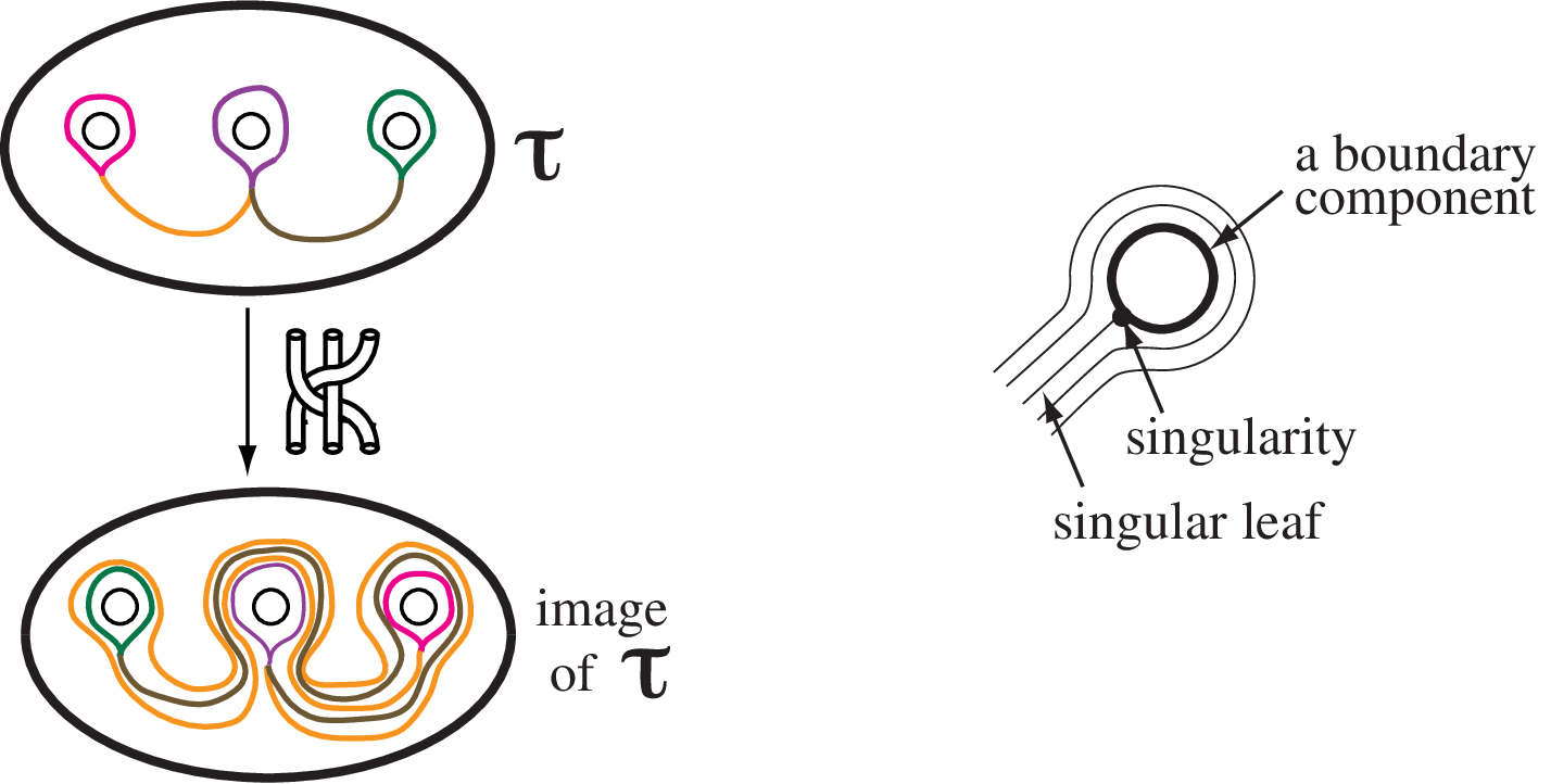
The invariant train track $\tau$ which carries the stable lamination $\ell^{s}$ for $\Phi$ is illustrated in Figure 4(left). The stable foliation $\mathcal{F}$ for $\Phi$ has a $1$ prong on each component of $\partial F$ and it has no singularity in the interior of $F$ . We consider the suspension flow induced on the mapping torus $N=F\times[0,1]/\sim,$ where $\sim$ identifies $(x,1)$ with $(\Phi(x),0)$ . One obtains the simple closed curve $c_{\alpha}\subset T_{\alpha}^{H}$ which is the closed orbit of the singularity of $\mathcal{F}$ on $\partial F\cap T_{\alpha}^{H}$ . Similarly one has the closed orbits $c_{\beta}\subset T_{\beta}^{H}$ , $c_{\gamma}\subset T_{\gamma}^{H}$ , see Figure 5(right). (One can draw these closed orbits by using the orbit of each cusp of $F\setminus\tau$ .) Let $\mathcal{L}^{s}\subset N$ be the suspended stable lamination which is constructed from $\ell^{s}\times I\subset F\times I$ by gluing $\ell^{s}\times\{1\}$ to $\ell^{s}\times\{0\}$ using $\Phi$ . By construction, $\mathcal{L}^{s}$ is carried by the branched surface $B_{\tau}$ which is obtained from $\tau\times I$ by gluing $\tau\times\{1\}$ to $\tau\times\{0\}$ using $\Phi$ . Notice that $c_{\alpha}$ , $c_{\beta}$ and $c_{\gamma}$ correspond to the branched loci of $B_{\tau}$ . By work of Fried [8] (see also work of Long-Oertel [18]), we may assume that the fiber $F_{(x,y,z)}$ is transverse to $\mathcal{L}^{s}$ . The stable lamination $\ell^{s}_{(x,y,z)}$ for $\Phi_{(x,y,z)}$ is given by the intersection $\mathcal{L}^{s}\cap F_{(x,y,z)}$ and $\ell^{s}_{(x,y,z)}$ is carried by the train track $B_{\tau}\cap F_{(x,y,z)}$ . This implies that $\mathcal{F}_{(x,y,z)}$ has no singularity in the interior of $F_{(x,y,z)}$ and we finish the proof of (4).

We consider the number of prongs of $\mathcal{F}_{(x,y,z)}$ at each component of $\partial_{\alpha}F_{(x,y,z)}$ . The boundary slope of each simple closed curve of $\partial_{\alpha}F_{(x,y,z)}$ is given by $\tfrac{-(y+z)}{x}$ . The desired number is equal to the intersection number

i([c_{-(y+z)/x}],[h(c_{\alpha})])=i([H(c_{-(y+z)/x})],[c_{\alpha}]),

where $c_{r}$ is a simple closed curve with slope $r\in{\mathbb{Q}}\cup\{\tfrac{1}{0}\}$ on $T_{\alpha}$ . Observe that $h(c_{\alpha})$ has the slope $\tfrac{1}{0}$ (see Figure 5). Hence

i([c_{-(y+z)/x}],[h(c_{\alpha})])=|1\cdot\tfrac{x}{\gcd(x,y+z)}+0\cdot\tfrac{y+z}{\gcd(x,y+z)}|=\tfrac{x}{\gcd(x,y+z)}.

This completes the proof of (1).

One verifies that $h(c_{\beta})$ and $h(c_{\gamma})$ have slopes $\tfrac{1}{0}$ and $\tfrac{-2}{1}$ respectively. By using the similar argument, one can prove (2),(3). $\Box$

We consider the orientability of $\mathcal{F}_{(x,y,z)}$ using Theorem 2.1. Alexander polynomial of $\mathcal{C}_{3}$ is

A(t_{1},t_{2},t_{3})=t_{1}t_{2}+t_{2}t_{3}+t_{3}t_{1}-t_{1}-t_{2}-t_{3}.

The following is a consequence of Proposition 7.3.10 in [12] which tells us that the relation between the Alexander polynomial of links and the characteristic polynomial of $\Phi_{*}:H_{1}(\varSigma;{\mathbb{R}})\rightarrow H_{1}(\varSigma;{\mathbb{R}})$ on fibers $\varSigma$ in the link exteriors.

Lemma 3.4.

The spectral radius of $(\Phi_{(x,y,z)})_{*}$ is the largest absolute value among roots of

A(t^{x},t^{y},t^{z})=t^{x+y}+t^{y+z}+t^{z+x}-t^{x}-t^{y}-t^{z}.

Proposition 3.5.

The pseudo-Anosov homeomorphism $\Phi_{(x,y,z)}$ is orientable if and only if $x$ and $y$ are even and $z$ is odd.

Proof. (If part.) Suppose that $x$ and $y$ are even and $z$ is odd. Then

P(t^{x},t^{y},t^{z})=A((-t)^{x},(-t)^{y},(-t)^{z}).

This implies that $\lambda(\Phi_{(x,y,z)})=\mathrm{sp}((\Phi_{(x,y,z)})_{*})$ . By Theorem 2.1 $\mathcal{F}_{(x,y,z)}$ is orientable.

(Only if part.) Suppose that $x$ or $y$ is odd. We may assume that $x$ is odd. The number of prongs of $\mathcal{F}_{(x,y,z)}$ at each component of $\partial_{\alpha}F_{(x,y,z)}$ equals $\tfrac{x}{\gcd(x,y+z)}$ which is odd. Thus $\mathcal{F}_{(x,y,z)}$ can not be orientable. $\Box$

3.3 Non-hyperbolic Dehn fillings

Let $M$ be a $3$ -manifold with boundary tori $T_{0},\cdots,T_{j}$ and let $r_{i}\in{\mathbb{Q}}\cup\infty$ be a slope on $T_{i}$ . Then $M(r_{0},r_{1},\cdots,r_{j})$ denotes the manifold obtained from $M$ by Dehn filling along the slope $r_{i}$ for each $i$ , that is $M(r_{0},r_{1},\cdots,r_{j})$ is the manifold attaching a solid torus $\widetilde{T}_{i}$ to $M$ along $T_{i}$ in such a way that $r_{i}$ bounds a disk in $\widetilde{T}_{i}$ .

Martelli and Petronio classified all the non-hyperbolic fillings of the magic manifold [20, Theorems 1.1, 1.2, 1.3]. We denote by $T_{0},T_{1},T_{2}$ , the boundary tori of $N=S^{3}\setminus\mathcal{N}(\mathcal{C}_{3})$ .

Theorem 3.6 ([20]).

(1)

$N(\tfrac{p}{q})$ is hyperbolic if and only if

\tfrac{p}{q}\notin\{\infty,-3,-2,-1,0\}.

(2)

$N(\tfrac{p}{q},\tfrac{r}{s})$ is hyperbolic if and only if

\tfrac{p}{q},\tfrac{r}{s}\notin\{\infty,-3,-2,-1,0\}\ \mbox{and}\ (\tfrac{p}{q},\tfrac{r}{s})\notin\{(1,1),(-4,\tfrac{-1}{2}),(\tfrac{-3}{2},\tfrac{-5}{2})\}.

As a corollary of Theorem 3.6 one has:

Corollary 3.7.

If $N(\tfrac{p}{q},\tfrac{r}{s},\tfrac{t}{u})$ is hyperbolic, then

\tfrac{p}{q},\tfrac{r}{s}\notin\{\infty,-3,-2,-1,0\}\ \mbox{and}\ (\tfrac{p}{q},\tfrac{r}{s})\notin\{(1,1),(-4,\tfrac{-1}{2}),(\tfrac{-3}{2},\tfrac{-5}{2})\}.

Let us consider the monodromy $\Phi_{(x,y,z)}:F_{(x,y,z)}\rightarrow F_{(x,y,z)}$ of the fibration on $N$ associated to a primitive fibered class $x\alpha+y\beta+z\gamma\in int(C_{\Delta})$ . Recall that $\mathrm{slope}(x\alpha+y\beta+z\gamma)=(\tfrac{-(y+z)}{x},\tfrac{-(z+x)}{y},\tfrac{-(x+y)}{z})$ , see (3.3). By capping each boundary component of $F_{(x,y,z)}$ , $\Phi_{(x,y,z)}$ extends to the monodromy $\overline{\Phi}_{(x,y,z)}$ with a closed fiber $\overline{F}_{(x,y,z)}$ of the fibration on $N(\frac{-(y+z)}{x},\frac{-(z+x)}{y},\frac{-(x+y)}{z})$ . If the stable foliation $\mathcal{F}_{(x,y,z)}$ has no $1$ prong on each component of $\partial F_{(x,y,z)}$ , then $\overline{\Phi}_{(x,y,z)}$ is pseudo-Anosov and $\lambda(\overline{\Phi}_{(x,y,z)})=\lambda(\Phi_{(x,y,z)})$ . If $\mathcal{F}_{(x,y,z)}$ has a $1$ prong on a component of $\partial F_{(x,y,z)}$ , then $\overline{\Phi}_{(x,y,z)}$ may not be pseudo-Anosov.

4 Hyperbolic Dehn fillings $N(\tfrac{-3}{2})$ , $N(\tfrac{-1}{2})$ and $N(2)$

4.1 Thurston norm balls of $N(\tfrac{-3}{2})$ , $N(\tfrac{-1}{2})$ and $N(2)$

Let $N(r)$ be the manifold obtained from $N$ by Dehn filling the cusp specified by $T_{\beta}$ along the slope $r\in\mathbb{Q}$ . Then there exists a natural injection $\iota_{\beta}:H_{2}(N(r),\partial N(r))\rightarrow H_{2}(N,\partial N)$ whose image equals

S_{\beta}(r)=\{(x,y,z)\in H_{2}(N,\partial N)\ |\ -ry=z+x\},

see [14]. By Theorem 3.6(1), $N(r)$ is hyperbolic if and only if $r\in{\mathbb{Q}}\setminus\{-3,-2,-1,0\}$ . Choose $r\in{\mathbb{Q}}\setminus\{-3,-2,-1,0\}$ , and assume that $a\in S_{\beta}(r)=\mathrm{Im}\,\iota_{\beta}$ is a fibered class of $H_{2}(N,\partial N)$ . Then $\overline{a}=\iota_{\beta}^{-1}(a)\in H_{2}(N(r),\partial N(r))$ is also a fibered class of $N(r)$ .

Similarly, when $N(r)$ is the manifold obtained from $N$ by Dehn filling the cusp specified by $T_{\alpha}$ or $T_{\gamma}$ along the slope $r$ , one has natural injections,

	$\displaystyle\iota_{\alpha}$	$\displaystyle:H_{2}(N(r),\partial N(r))\to H_{2}(N,\partial N),$
	$\displaystyle\iota_{\gamma}$	$\displaystyle:H_{2}(N(r),\partial N(r))\to H_{2}(N,\partial N)$

such that their images are

	$\displaystyle S_{\alpha}(r)$	$\displaystyle=\{(x,y,z)\in H_{2}(N,\partial N)\,\|\,-rx=y+z\},$
	$\displaystyle S_{\gamma}(r)$	$\displaystyle=\{(x,y,z)\in H_{2}(N,\partial N)\,\|\,-rz=x+y\}.$

We set

$\displaystyle\mathfrak{a}$	$\displaystyle=$	$\displaystyle 2\alpha+2\beta+\gamma,\hskip 5.69054pt\mathfrak{b}=\alpha+2\beta+2\gamma,$
$\displaystyle\mathfrak{p}$	$\displaystyle=$	$\displaystyle\alpha+2\beta,\ \hskip 25.60747pt\mathfrak{q}=2\beta+\gamma,$
$\displaystyle\mathfrak{r}$	$\displaystyle=$	$\displaystyle\alpha+\beta-\gamma,\ \hskip 11.38109pt\mathfrak{s}=\alpha-\beta.$

For $k,\ell\in{\mathbb{Z}}$ , we have

\begin{split}\mathrm{slope}(k\mathfrak{a}+\ell\mathfrak{b})&=(\tfrac{-3k-4\ell}{2k+\ell},\tfrac{-3}{2},\tfrac{-4k-3\ell}{k+2\ell}),\\ \mathrm{slope}(k\mathfrak{p}+\ell\mathfrak{q})&=(\tfrac{-2k-3\ell}{k},\tfrac{-1}{2},\tfrac{-3k-2\ell}{\ell}),\\ \mathrm{slope}(k\mathfrak{r}+\ell\mathfrak{s})&=(\tfrac{\ell}{k+\ell},\tfrac{-\ell}{k-\ell},2),\ \mbox{and}\end{split}

(4.1)

\begin{split}k\mathfrak{a}+\ell\mathfrak{b}&=(2k+\ell)\alpha+(2k+2\ell)\beta+(k+2\ell)\gamma\in\iota_{\beta}(H_{2}(N(\tfrac{-3}{2}),\partial N(\tfrac{-3}{2}))),\\ k\mathfrak{p}+\ell\mathfrak{q}&=k\alpha+(2k+2\ell)\beta+\ell\gamma\in\iota_{\beta}(H_{2}(N(\tfrac{-1}{2}),\partial N(\tfrac{-1}{2}))),\\ k\mathfrak{r}+\ell\mathfrak{s}&=(k+\ell)\alpha+(k-\ell)\beta-k\gamma\in\iota_{\gamma}(H_{2}(N(2),\partial N(2))).\end{split}

(4.2)

It is easy to check that $\{\overline{\mathfrak{a}},\overline{\mathfrak{b}}\}$ , $\{\overline{\mathfrak{p}},\overline{\mathfrak{q}}\}$ and $\{\overline{\mathfrak{r}},\overline{\mathfrak{s}}\}$ are bases of $H_{2}(N(\tfrac{-3}{2}),\partial N(\tfrac{-3}{2});{\mathbb{Z}})$ , $H_{2}(N(\tfrac{-1}{2}),\partial N(\tfrac{-1}{2});{\mathbb{Z}})$ and $H_{2}(N(2),\partial N(2);{\mathbb{Z}})$ respectively.

Note that $\gcd(k,\ell)=1$ if and only if $k\mathfrak{a}+\ell\mathfrak{b}$ , $k\mathfrak{p}+\ell\mathfrak{q}$ and $k\mathfrak{r}+\ell\mathfrak{s}$ are primitive integral classes of $H_{2}(N,\partial N;{\mathbb{R}})$ . All $k\mathfrak{a}+\ell\mathfrak{b},k\mathfrak{p}+\ell\mathfrak{q},k\mathfrak{r}+\ell\mathfrak{s}$ are fibered classes in $int(C_{\Delta})$ for $k>0$ and $-k<\ell<k$ .

We first focus on the topological types of fibers for primitive fibered classes in $int(C_{\Delta})$ . Let $\varSigma_{g,p}$ be a compact orientable surface of genus $g$ with $p$ boundary components.

Lemma 4.1.

Suppose that $k>0$ , $-k<\ell<k$ and $\gcd(k,\ell)=1$ .

(1): $F_{k\mathfrak{a}+\ell\mathfrak{b}}=\varSigma_{k-2,k+\ell+6}$ if $\gcd(2k+\ell,5)=5$ or $\gcd(5,k+2\ell)=5$ . Otherwise $F_{k\mathfrak{a}+\ell\mathfrak{b}}=\varSigma_{k,k+\ell+2}$ .
(2): $F_{k\mathfrak{p}+\ell\mathfrak{q}}=\varSigma_{k-1,k+\ell+4}$ if $\gcd(k,3)=3$ or $\gcd(3,\ell)=3$ . Otherwise $F_{k\mathfrak{p}+\ell\mathfrak{q}}=\varSigma_{k,k+\ell+2}$ .
(3): $F_{k\mathfrak{r}+\ell\mathfrak{s}}=\varSigma_{k,k+2}$ .

Proof of (1). By Lemma 3.1,

$\displaystyle\sharp(\partial F_{k\mathfrak{a}+\ell\mathfrak{b}})$	$\displaystyle=$	$\displaystyle\gcd(2k+\ell,3k+4\ell)+\gcd(2k+2\ell,3k+3\ell)+\gcd(4k+3\ell,k+2\ell)$
	$\displaystyle=$	$\displaystyle\gcd(2k+\ell,5k)+k+\ell+\gcd(5\ell,k+2\ell)$
	$\displaystyle=$	$\displaystyle\gcd(2k+\ell,5)+k+\ell+\gcd(5,k+2\ell).$

The last equality holds since $\gcd(k,\ell)=1$ . The following 3 cases can occur.

(1): $\gcd(2k+\ell,5)=1$ and $\gcd(5,k+2\ell)=1$ .
(2): $\gcd(2k+\ell,5)=5$ and $\gcd(5,k+2\ell)=1$ .
(3): $\gcd(2k+\ell,5)=1$ and $\gcd(5,k+2\ell)=5$ .

In the case (1), the genus $g$ of $F_{k\mathfrak{a}+\ell\mathfrak{b}}$ must satisfy

-(2-2g-k-\ell-2)=\|k\mathfrak{a}+\ell\mathfrak{b}\|=3k+\ell

(see (3.1)). Thus $g=k$ and $F_{k\mathfrak{a}+\ell\mathfrak{b}}=\varSigma_{k,k+\ell+2}$ . In the cases (2) and (3), $F_{k\mathfrak{a}+\ell\mathfrak{b}}=\varSigma_{k-2,k+\ell+6}$ .

The proof of claims (2), (3) of the lemma is similar. $\Box$

Lemma 4.2.

Suppose that $k>0$ and $-k<\ell<k$ .

(1): $F_{k\mathfrak{a}+\ell\mathfrak{b}}=F_{\ell\mathfrak{a}+k\mathfrak{b}}$ and $\lambda(k\mathfrak{a}+\ell\mathfrak{b})=\lambda(\ell\mathfrak{a}+k\mathfrak{b})$ .
(2): $F_{k\mathfrak{p}+\ell\mathfrak{q}}=F_{\ell\mathfrak{p}+k\mathfrak{q}}$ and $\lambda(k\mathfrak{p}+\ell\mathfrak{q})=\lambda(\ell\mathfrak{p}+k\mathfrak{q})$ .

Proof. (1) By the symmetry of the Thurston norm ball of $N$ , it is not hard to see that the topological type of the minimal representative (resp. the dilatation) for $\ell\mathfrak{a}+k\mathfrak{b}=(2\ell+k)\alpha+(2\ell+2k)\beta+(\ell+2k)\gamma$ is same as the one for $k\mathfrak{a}+\ell\mathfrak{b}=(2k+\ell)\alpha+(2k+2\ell)\beta+(k+2\ell)\gamma$ .

The proof of (2) is similar. $\Box$

We make a remark that it is not true in general that $F_{k\mathfrak{r}+\ell\mathfrak{s}}=F_{\ell\mathfrak{r}+k\mathfrak{s}}$ and $\lambda(k\mathfrak{r}+\ell\mathfrak{s})=\lambda(\ell\mathfrak{r}+k\mathfrak{s})$ for $k>0$ and $-k<\ell<k$ . We do not use this remark in the rest of the paper.

Lemma 4.3.

Suppose that $0<\ell<k$ and $\gcd(k,\ell)=1$ .

(1): The genus of $F_{k\mathfrak{a}+\ell\mathfrak{b}}$ equals the one of $F_{k\mathfrak{a}-\ell\mathfrak{b}}$ .
(2): The genus of $F_{k\mathfrak{p}+\ell\mathfrak{q}}$ equals the one of $F_{k\mathfrak{p}-\ell\mathfrak{q}}$ .
(3): The genera of $F_{k\mathfrak{r}+\ell\mathfrak{s}}$ and $F_{k\mathfrak{r}-\ell\mathfrak{s}}$ equal $k$

Proof. (1) By Lemma 4.1(1), the genus of $F_{k\mathfrak{a}\pm\ell\mathfrak{b}}$ equals $k-2$ if $\gcd(2k\pm\ell,5)=5$ or $\gcd(5,k\pm 2\ell)=5$ . Otherwise its genus equals $k$ . It is easy to check that

•

$\gcd(2k+\ell,5)=5$ if and only if $\gcd(5,k-2\ell)=5$ .
•

$\gcd(2k-\ell,5)=5$ if and only if $\gcd(5,k+2\ell)=5$ .

This implies the desired claim (1).

By using the similar argument, one can prove (2). The claim (3) is obvious from Lemma 4.1(3). $\Box$

Lemma 4.4.

Suppose that $0<\ell<k$ . Then

\lambda(k\mathfrak{a}\pm\ell\mathfrak{b})=\lambda(k\mathfrak{p}\pm\ell\mathfrak{q})=\lambda(k\mathfrak{r}\pm\ell\mathfrak{s})=\lambda_{(k,\ell)}.

Proof. We use Theorem 3.2. The dilatations of $k\mathfrak{a}\pm\ell\mathfrak{b}$ and $k\mathfrak{p}\pm\ell\mathfrak{q}$ are the largest real root of

f_{(2k\pm\ell,2k\pm 2\ell,k\pm 2\ell)}(t)=f_{(k,2k\pm 2\ell,\pm\ell)}(t)=(t^{k\pm\ell}+1)(t^{2k}-t^{k+\ell}-t^{k}-t^{k-\ell}+1).

The dilatation of $k\mathfrak{r}\pm\ell\mathfrak{s}$ is the largest real root of

f_{(k\pm\ell,k\mp\ell,-k)}(t)=(t^{k}+1)(t^{2k}-t^{k+\ell}-t^{k}-t^{k-\ell}+1).

Since the absolute values of all roots of $t^{k\pm\ell}+1$ and $t^{k}+1$ are equal to $1$ , one finishes the proof. $\Box$

By Proposition 3.5 and (4.2), we immediately obtain the following.

Corollary 4.5.

Suppose that $k>0$ , $-k<\ell<k$ and $\gcd(k,\ell)=1$ .

(1): The monodromy of the fibration associated to $k\mathfrak{a}+\ell\mathfrak{b}$ on $N$ is orientable if and only if $k$ is odd and $\ell$ is even.
(2): The monodromy of the fibration associated to $k\mathfrak{p}+\ell\mathfrak{q}$ on $N$ is orientable if and only if $k$ is even and $\ell$ is odd.
(3): The monodromy of the fibration associated to $k\mathfrak{r}+\ell\mathfrak{s}$ on $N$ is orientable if and only if both $k$ and $\ell$ are odd.

The following can be obtained from Proposition 3.3

Corollary 4.6.

Suppose that $k>0$ , $-k<\ell<k$ and $\gcd(k,\ell)=1$ .

(1)

The singularity data of the monodromy of the fibration associated to $k\mathfrak{a}+\ell\mathfrak{b}$ on $N$ is given by

(\underbrace{\tfrac{2k+\ell}{\gcd(2k+\ell,5)}-2,\cdots,\tfrac{2k+\ell}{\gcd(2k+\ell,5)}-2}_{\gcd(2k+\ell,5)},\underbrace{\tfrac{2k-\ell}{\gcd(5,k+2\ell)}-2,\cdots,\tfrac{2k-\ell}{\gcd(5,k+2\ell)}}_{\gcd(5,k+2\ell)}).

(2)

The singularity data of the monodromy of the fibration associated to $k\mathfrak{p}+\ell\mathfrak{q}$ on $N$ is given by

(\underbrace{\tfrac{k}{\gcd(k,3)}-2,\cdots,\tfrac{k}{\gcd(k,3)}-2}_{\gcd(k,3)},\underbrace{\tfrac{3k}{\gcd(3,\ell)}-2,\cdots,\tfrac{3k}{\gcd(3,\ell)}-2}_{\gcd(3,\ell)}).

(3)

The singularity data of the monodromy of the fibration associated to $k\mathfrak{r}+\ell\mathfrak{s}$ on $N$ is given by

(k+\ell-2,k-\ell-2,\underbrace{2,\cdots,2}_{k}).

Remark 4.7.

(1): The stable foliation for the monodromy of the fibration associated to $k\mathfrak{a}+\ell\mathfrak{b}$ (resp. $k\mathfrak{p}+\ell\mathfrak{q}$ ) has $2$ prongs on each boundary component on $T_{\beta}$ . (Hence there is no singular leaf on $\partial_{\beta}F_{k\mathfrak{a}+\ell\mathfrak{b}}$ (resp. $\partial_{\beta}F_{k\mathfrak{p}+\ell\mathfrak{q}}$ ).)
(2): The stable foliation for the monodromy of the fibration associated to $k\mathfrak{r}+\ell\mathfrak{s}$ has $4$ prongs on each boundary component on $T_{\gamma}$ .

Lemma 4.8.

Suppose that $k>0$ , $-k<\ell<k$ and $\gcd(k,\ell)=1$ .

(1): The stable foliation for the monodromy of the fibration associated to $k\mathfrak{a}+\ell\mathfrak{b}$ has a $1$ prong on a boundary component if and only if $(k,\ell)\in\{(2,\pm 1),(3,\pm 1),(4,\pm 3)\}$ .
(2): The stable foliation for the monodromy of the fibration associated to $k\mathfrak{p}+\ell\mathfrak{q}$ has a $1$ prong on a boundary component if and only if $(k,\ell)\in\{(1,0),(3,\pm 1),(3,\pm 2)\}$ .
(3): The stable foliation for the monodromy of the fibration associated to $k\mathfrak{r}+\ell\mathfrak{s}$ has a $1$ prong on a boundary component if and only if $k+\ell=1$ or $k-\ell=1$ .

Proof. (1) By Corollary 4.6, the stable foliation of the monodromy for $k\mathfrak{a}+\ell\mathfrak{b}$ has a $1$ prong if and only if $\tfrac{2k+\ell}{\gcd(2k+\ell,5)}=1$ or $\tfrac{2k-\ell}{\gcd(5,k+2\ell)}=1$ .

Suppose that $\tfrac{2k+\ell}{\gcd(2k+\ell,5)}=1$ . Clearly $\gcd(2k+\ell,5)=1$ or $5$ . If $\gcd(2k+\ell,5)=1$ , then $2k+\ell=1$ . Since $-k<\ell<k$ , one has $-k<-2k+1<k$ which implies that $\tfrac{1}{3}<k<1$ . This does not occur since $k$ is an integer. If $\gcd(2k+\ell,5)=5$ , then $2k+\ell=5$ . Since $-k<\ell<k$ , one has $-k<5-2k<k$ which implies $\tfrac{5}{3}<k<5$ . Hence $(k,\ell)\in\{(2,1),(3,-1),(4,-3)\}$ .

Suppose that $\tfrac{2k-\ell}{\gcd(5,k+2\ell)}=1$ . In this case one sees that $(k,\ell)\in\{(2,-1),(3,1),(4,3)\}$ . This completes the proof of (1).

By using the same argument one can prove (2),(3). $\Box$

Remark 4.9.

Suppose that $k>0$ , $-k<\ell<k$ and $\gcd(k,\ell)=1$ . By Lemma 4.8 and Corollary 3.7, we see that:

(1): $N(\tfrac{-3k-4\ell}{2k+\ell},\tfrac{-3}{2},\tfrac{-4k-3\ell}{k+2\ell})$ is non-hyperbolic for $(k,\ell)\in\{(2,\pm 1),(3,\pm 1),(4,\pm 3)\}$ . Otherwise it is hyperbolic.
(2): $N(\tfrac{-2k-3\ell}{k},\tfrac{-1}{2},\tfrac{-3k-2\ell}{\ell})$ is non-hyperbolic for $(k,\ell)\in\{(1,0),(3,\pm 1),(3,\pm 2)\}$ . Otherwise it is hyperbolic.
(3): Suppose that $k+\ell=1$ or $k-\ell=1$ . Then we have the following. $N(\tfrac{\ell}{k+\ell},\tfrac{-\ell}{k-\ell},2)$ is non-hyperbolic if $(k,\ell)\in\{(2,\pm 1),(3,\pm 2),(4,\pm 3)\}$ and it is hyperbolic if $(k,\ell)\notin\{(2,\pm 1),(3,\pm 2),(4,\pm 3)\}$ . Suppose that $k+\ell\neq 1$ and $k-\ell\neq 1$ . Then $N(\tfrac{\ell}{k+\ell},\tfrac{-\ell}{k-\ell},2)$ is hyperbolic.

For each of $N(\tfrac{-3}{2})$ , $N(\tfrac{-1}{2})$ and $N(2)$ , its Thurston norm ball of radius $2$ is a rectangle with vertices $(k,\ell)=(\pm 1,\pm 1)$ illustrated in Figure 6. By using (3.1) we see that for $k,\ell\in{\mathbb{R}}$ ,

\|k\overline{\mathfrak{a}}+\ell\overline{\mathfrak{b}}\|=\|k\overline{\mathfrak{p}}+\ell\overline{\mathfrak{q}}\|=\|k\overline{\mathfrak{r}}+\ell\overline{\mathfrak{s}}\|=\max\{2|k|,2|\ell|\}.

(4.3)

The following lemma asserts that fibered faces for $N(\tfrac{-3}{2})$ and $N(\tfrac{-1}{2})$ has a symmetry. Thus, for the study of monodromies on fibrations on $N(\tfrac{-3}{2})$ (resp. $N(\tfrac{-1}{2})$ ), it is enough to consider the open cone over an arbitrary picked fibered face.

Lemma 4.10.

Suppose that $k>0$ and $-k<\ell<k$ .

(1): $F_{k\overline{\mathfrak{a}}+\ell\overline{\mathfrak{b}}}=F_{\ell\overline{\mathfrak{a}}+k\overline{\mathfrak{b}}}$ and $\lambda(k\overline{\mathfrak{a}}+\ell\overline{\mathfrak{b}})=\lambda(\ell\overline{\mathfrak{a}}+k\overline{\mathfrak{b}})$ .
(2): $F_{k\overline{\mathfrak{p}}+\ell\overline{\mathfrak{q}}}=F_{\ell\overline{\mathfrak{p}}+k\overline{\mathfrak{q}}}$ and $\lambda(k\overline{\mathfrak{p}}+\ell\overline{\mathfrak{q}})=\lambda(\ell\overline{\mathfrak{p}}+k\overline{\mathfrak{q}})$ .

Proof. See Lemma 4.2 and Remark 4.7(1). $\Box$

Let us fix an open cones

$\displaystyle int(C_{\Delta(-3/2)})$	$\displaystyle=$	$\displaystyle\{k\overline{\mathfrak{a}}+\ell\overline{\mathfrak{b}}\ \|\ k>0,\ -k<\ell<k\}\subset H_{2}(N(\tfrac{-3}{2}),\partial N(\tfrac{-3}{2});{\mathbb{R}}),$
$\displaystyle int(C_{\Delta(-1/2)})$	$\displaystyle=$	$\displaystyle\{k\overline{\mathfrak{p}}+\ell\overline{\mathfrak{q}}\ \|\ k>0,\ -k<\ell<k\}\subset H_{2}(N(\tfrac{-1}{2}),\partial N(\tfrac{-1}{2});{\mathbb{R}}),$
$\displaystyle int(C_{\Delta(2)})$	$\displaystyle=$	$\displaystyle\{k\overline{\mathfrak{r}}+\ell\overline{\mathfrak{s}}\ \|\ k>0,\ -k<\ell<k\}\subset H_{2}(N(2),\partial N(2);{\mathbb{R}}).$

Lemmas 4.11 and 4.12 tell us that it is enough to consider the fibered classes of $int(C_{\Delta(r)})$ for $0<\ell<k$ .

Lemma 4.11.

Suppose that $0<\ell<k$ and $\gcd(k,\ell)=1$ .

(1): $F_{k\overline{\mathfrak{a}}\pm\ell\overline{\mathfrak{b}}}=\varSigma_{k-2,6}$ if $\gcd(2k+\ell,5)=5$ or $\gcd(5,k+2\ell)=5$ . Otherwise $F_{k\overline{\mathfrak{a}}+\ell\overline{\mathfrak{b}}}=\varSigma_{k,2}$ .
(2): $F_{k\overline{\mathfrak{p}}\pm\ell\overline{\mathfrak{q}}}=\varSigma_{k-1,4}$ if $\gcd(k,3)=3$ or $\gcd(3,\ell)=3$ . Otherwise $F_{k\overline{\mathfrak{p}}+\ell\overline{\mathfrak{q}}}=\varSigma_{k,2}$ .
(3): $F_{k\overline{\mathfrak{r}}\pm\ell\overline{\mathfrak{s}}}=\varSigma_{k,2}$ .

Proof. The number of the components of $\partial_{\beta}F_{k\mathfrak{a}+\ell\mathfrak{b}}$ equals $k+\ell$ . By Lemma 4.1(1), we have the desired claim (1). One can prove (2),(3) by using Lemma 4.1(2),(3) respectively. $\Box$

Lemma 4.12.

Suppose that $0<\ell<k$ . Then

\lambda(k\overline{\mathfrak{a}}\pm\ell\overline{\mathfrak{b}})=\lambda(k\overline{\mathfrak{p}}\pm\ell\overline{\mathfrak{q}})=\lambda(k\overline{\mathfrak{r}}\pm\ell\overline{\mathfrak{s}})=\lambda_{(k,\ell)}.

Proof. See Lemma 4.4 and Remark 4.7. $\Box$

Proposition 4.13.

Let $r\in\{\tfrac{-3}{2},\tfrac{-1}{2},2\}$ . The minimum of $\mathrm{Ent}:int(C_{\Delta(r)})\rightarrow{\mathbb{R}}$ equals $2\log\lambda_{(1,0)}=2\log\bigl(\tfrac{3+\sqrt{5}}{2}\bigr)$ . The minimizer is given by $\overline{\mathfrak{a}}$ if $r=\tfrac{-3}{2}$ , $\overline{\mathfrak{p}}$ if $r=\tfrac{-1}{2}$ and $\overline{\mathfrak{r}}$ if $r=2$ .

Proof. Recall that $\mathrm{Ent}$ is constant on each ray thorough the origin and it has the minimum at a unique ray. By Lemma 4.12 and (4.3), the ray which reaches the minimum must satisfy $\ell=0$ . As a representative which lies on such a ray, we take $k=1$ and $\ell=0$ . This together with Theorem 3.2 implies that $\min\mathrm{Ent}=2\log\lambda_{(1,0)}=2\log\bigl(\tfrac{3+\sqrt{5}}{2}\bigr)$ . $\Box$

Remark 4.14.

The monodromies of the fibrations associated to $\overline{\mathfrak{a}}$ (resp. $\overline{\mathfrak{p}}$ ) on $N(\tfrac{-3}{2})$ (resp. $N(\tfrac{-1}{2})$ ) are intriguing examples.

(1): $N(\tfrac{-3}{2})$ admits a fiber of genus $1$ with $2$ boundary components corresponding to $\overline{\mathfrak{a}}$ . Its monodromy $\Phi:\varSigma_{1,2}\rightarrow\varSigma_{1,2}$ has $2$ prongs on each boundary component. Thus $\Phi$ extends to the monodromy $\overline{\Phi}:\varSigma_{1,1}\rightarrow\varSigma_{1,1}$ of the fibration on $N(\tfrac{-3}{2},\tfrac{-3}{2})$ (which is the figure- $8$ knot sister manifold, see [20, Table A.2]) by capping the boundary component of $\varSigma_{1,2}$ on $T_{\alpha}$ . It is well-known that $\overline{\Phi}$ realizes the minimal dilatation $\tfrac{3+\sqrt{5}}{2}$ among pseudo-Anosovs on $\varSigma_{1,1}$ .
(2): $N(\tfrac{-1}{2})$ admits a fiber of genus $0$ with $4$ boundary components corresponding to $\overline{\mathfrak{p}}$ . Its monodromy $\Phi$ fixes a boundary component, and hence it can be considered that $\Phi$ is a pseudo-Anosov homeomorphism on a $3$ -punctured disk $D_{3}$ . This monodromy $\Phi$ realizes the minimal dilatation $\delta(D_{3})=\tfrac{3+\sqrt{5}}{2}$ among pseudo-Anosovs on $D_{3}$ .

4.2 Property of algebraic integers $\lambda_{(k,\ell)}$

Lemma 4.15.

Suppose that $1<\ell+1<k$ and $\gcd(k,\ell)=1$ . Then $\lambda_{(k+1,\ell)}<\lambda_{(k,\ell)}<\lambda_{(k,\ell+1)}$ .

Proof. The ray which attains the minimum of $\mathrm{Ent}:int(C_{\Delta(r)})\rightarrow{\mathbb{R}}$ satisfies $\ell=0$ . Recall that $\tfrac{1}{\mathrm{ent}(\cdot)}:int(C_{\Delta(r)}(\mathbb{Q}))\rightarrow{\mathbb{R}}$ is strictly concave. Thus one has

\log\lambda_{(k,\tfrac{k\ell}{k+1})}<\log\lambda_{(k,\ell)}<\log\lambda_{(k,\ell+1)}.

The inequality $\log\lambda_{(k+1,\ell)}<\log\lambda_{(k,\ell)}$ holds since

\log\lambda_{(k+1,\ell)}=\mathrm{ent}((k+1)\overline{\mathfrak{a}}+\ell\overline{\mathfrak{b}})=\tfrac{k}{k+1}\mathrm{ent}(k\overline{\mathfrak{a}}+\tfrac{k\ell}{k+1}\overline{\mathfrak{b}})=\tfrac{k}{k+1}\log\lambda_{(k,\tfrac{k\ell}{k+1})}<\log\lambda_{(k,\tfrac{k\ell}{k+1})}.

Hence $\log\lambda_{(k+1,\ell)}<\log\lambda_{(k,\ell)}<\log\lambda_{(k,\ell+1)}$ . $\Box$

Lemma 4.16.

For any fixed $\ell>0$ ,

\lim_{k\to\infty}k\log\lambda_{(k,\ell)}=\log\lambda_{(1,0)}=\log(\tfrac{3+\sqrt{5}}{2}).

Proof. The ray through $k\overline{\mathfrak{a}}+\ell\overline{\mathfrak{b}}$ from the origin goes to the ray through $\overline{\mathfrak{a}}$ if $k$ goes to $\infty$ . Hence

\lim_{k\to\infty}\mathrm{Ent}(k\overline{\mathfrak{a}}+\ell\overline{\mathfrak{b}})=\lim_{k\to\infty}2k\log\lambda_{(k,\ell)}=\mathrm{Ent}(\overline{\mathfrak{a}})=2\log\lambda_{(1,0)}.

This completes the proof. $\Box$

Proposition 4.17.

If $\lambda_{(k+1,\ell)}<\lambda_{(k,1)}$ for some $k\geq\ell\geq 2$ , then $\lambda_{(k+2,\ell)}<\lambda_{(k+1,1)}$ .

Proof. We denote the homology class $k\overline{\mathfrak{a}}+\ell\overline{\mathfrak{b}}$ by $(k,\ell)$ . Since $\mathrm{Ent}$ is constant on each ray thorough the origin, $k\mathrm{ent}(k,\ell)=\mathrm{ent}(1,\tfrac{\ell}{k})$ . One takes $4$ points

p_{1}=(1,\tfrac{1}{k+1}),\ p_{2}=(1,\tfrac{1}{k}),\ p_{3}=(1,\tfrac{\ell}{k+2}),\ p_{4}=(1,\tfrac{\ell}{k+1}),

see Figure 7. We have $\tfrac{1}{k+1}<\tfrac{1}{k}<\tfrac{2}{k+2}\leq\tfrac{\ell}{k+2}<\tfrac{\ell}{k+1}$ . Let us set $t,t^{\prime}$ and $c$ as follows.

\begin{split}0<t&=\frac{|p_{3}-p_{2}|}{|p_{4}-p_{2}|}=\frac{(k+1)(k\ell-k-2)}{(k+2)(k\ell-k-1)}<1,\\ 0<t&{}^{\prime}=\frac{|p_{3}-p_{2}|}{|p_{3}-p_{1}|}=\frac{|p_{4}-p_{2}|}{|p_{3}-p_{1}|}t=\frac{(k+2)(k\ell-k-1)}{k(k\ell-k+\ell-2)}t<1,\\ 1<c&=\frac{(k+2)(k\ell-k-1)}{k(k\ell-k+\ell-2)}.\end{split}

(4.4)

(Hence $t^{\prime}=ct$ .) Then

	$\displaystyle\|p_{3}-p_{2}\|:\|p_{4}-p_{3}\|$	$\displaystyle=$	$\displaystyle t:1-t,$
	$\displaystyle\|p_{3}-p_{2}\|:\|p_{2}-p_{1}\|$	$\displaystyle=$	$\displaystyle ct:1-ct.$

These ratios together with Theorem 2.3 imply that

	$\displaystyle\frac{1}{(k+2)\mathrm{ent}(k+2,\ell)}>(1-t)\frac{1}{k\mathrm{ent}(k,1)}+t\frac{1}{(k+1)\mathrm{ent}(k+1,\ell)},$		(4.5)
	$\displaystyle\frac{1}{k\mathrm{ent}(k,1)}>ct\frac{1}{(k+1)\mathrm{ent}(k+1,1)}+(1-ct)\frac{1}{(k+2)\mathrm{ent}(k+2,\ell)}.$		(4.6)

By (4.5) and by the assumption $\mathrm{ent}(k,1)>\mathrm{ent}(k+1,\ell)$ ,

$\displaystyle\frac{1}{(k+2)\mathrm{ent}(k+2,\ell)}$	$\displaystyle>$	$\displaystyle(1-t)\frac{1}{k\mathrm{ent}(k,1)}+t\frac{1}{(k+1)\mathrm{ent}(k+1,\ell)}$
	$\displaystyle>$	$\displaystyle(1-t)\frac{1}{k\mathrm{ent}(k,1)}+t\frac{1}{(k+1)\mathrm{ent}(k,1)}$
	$\displaystyle=$	$\displaystyle\frac{k+1-t}{k+1}\frac{1}{k\mathrm{ent}(k,1)}$
	$\displaystyle>$	$\displaystyle\frac{k+1-t}{k+1}\Big\{ct\frac{1}{(k+1)\mathrm{ent}(k+1,1)}+(1-ct)\frac{1}{(k+2)\mathrm{ent}(k+2,\ell)}\Big\}.$

The last inequality is given by (4.6). Hence

\displaystyle\Big\{\frac{1}{k+2}\ -\frac{(k+1-t)(1-ct)}{(k+1)(k+2)}\Big\}\frac{1}{\mathrm{ent}(k+2,\ell)}>\frac{(k+1-t)ct}{(k+1)^{2}}\frac{1}{\mathrm{ent}(k+1,1)},

which gives, by calculation,

\displaystyle\frac{(k+1-t)c+1}{k+2}\frac{1}{\mathrm{ent}(k+2,\ell)}>\frac{(k+1-t)c}{k+1}\frac{1}{\mathrm{ent}(k+1,1)}.

Thus

\displaystyle\mathrm{ent}(k+2,\ell)<\Big\{\frac{k+1}{(k+1-t)c}\Big\}\Big\{\frac{(k+1-t)c+1}{k+2}\Big\}\mathrm{ent}(k+1,1).

For the proof of the claim it is enough to verify the equality $\Big\{\frac{k+1}{(k+1-t)c}\Big\}\Big\{\frac{(k+1-t)c+1}{k+2}\Big\}=1$ . Clearly,

			$\displaystyle\Big\{\frac{k+1}{(k+1-t)c}\Big\}\Big\{\frac{(k+1-t)c+1}{k+2}\Big\}=1$
		$\displaystyle\Leftrightarrow$	$\displaystyle(k+1)\{(k+1-t)c+1\}=(k+2)(k+1-t)c$
		$\displaystyle\Leftrightarrow$	$\displaystyle(k+1)(k+1-t)c+k+1=(k+2)(k+1-t)c$
		$\displaystyle\Leftrightarrow$	$\displaystyle k+1=(k+1-t)c$
		$\displaystyle\Leftrightarrow$	$\displaystyle c=\frac{k+1}{k+1-t}.$

One can verify the last equality $c=\frac{k+1}{k+1-t}$ by substituting the constants $t$ and $c$ given by (4.4). $\Box$

4.3 Fibrations of manifolds obrained from $N(\tfrac{-1}{2}),N(\tfrac{-3}{2})$ and $N(2)$ by Dehn filling two cusps

As a consequence of Lemma 4.8, we see the following.

Remark 4.18.

If $(k,\ell)\notin\{(2,\pm 1),(3,\pm 1),(4,\pm 3)\}$ , then the monodromy $\Phi_{k\mathfrak{a}+\ell\mathfrak{b}}:F_{k\mathfrak{a}+\ell\mathfrak{b}}\rightarrow F_{k\mathfrak{a}+\ell\mathfrak{b}}$ of the fibration associated to $k\mathfrak{a}+\ell\mathfrak{b}$ on $N$ extends to the monodromy $\overline{\Phi}_{k\mathfrak{a}+\ell\mathfrak{b}}:\overline{F}_{k\mathfrak{a}+\ell\mathfrak{b}}\rightarrow\overline{F}_{k\mathfrak{a}+\ell\mathfrak{b}}$ of the fibration on $N(\tfrac{-3k-4\ell}{2k+\ell},\tfrac{-3}{2},\tfrac{-4k-3\ell}{k+2\ell})$ with the dilatation $\lambda_{(k,\ell)}(=\lambda(\Phi_{k\mathfrak{a}+\ell\mathfrak{b}}))$ . Similarly, if $(k,\ell)\notin\{(1,0),(3,\pm 1),(3,\pm 2)\}$ (resp. if $k+\ell\neq 1$ and $k-\ell\neq 1$ ), then the monodromy $\Phi_{k\mathfrak{p}+\ell\mathfrak{q}}$ (resp. $\Phi_{k\mathfrak{r}+\ell\mathfrak{s}}$ ) of the fibration associated to $k\mathfrak{p}+\ell\mathfrak{q}$ (resp. $k\mathfrak{r}+\ell\mathfrak{s}$ ) on $N$ extends to the monodromy $\overline{\Phi}_{k\mathfrak{p}+\ell\mathfrak{q}}$ (resp. $\overline{\Phi}_{k\mathfrak{r}+\ell\mathfrak{s}}$ ) of the fibration on $N(\tfrac{-2k-3\ell}{k},\tfrac{-1}{2},\tfrac{-3k-2\ell}{\ell})$ (resp. $N(\tfrac{\ell}{k+\ell},\tfrac{-\ell}{k-\ell},2)$ ) with the dilatation $\lambda_{(k,\ell)}$ .

Let $\overline{\phi}_{k\mathfrak{a}+\ell\mathfrak{b}}$ , $\overline{\phi}_{k\mathfrak{p}+\ell\mathfrak{q}}$ and $\overline{\phi}_{k\mathfrak{r}+\ell\mathfrak{s}}$ be elements of $\mathrm{Mod}(\varSigma_{g})$ containing $\overline{\Phi}_{k\mathfrak{a}+\ell\mathfrak{b}}$ , $\overline{\Phi}_{k\mathfrak{p}+\ell\mathfrak{q}}$ and $\overline{\Phi}_{k\mathfrak{r}+\ell\mathfrak{s}}$ as a representative.

Proposition 4.19.

For any fixed integer $\ell>0$ , we have the following.

(1): $\displaystyle\lim_{\begin{subarray}{c}k\to\infty\\ \gcd(k,\ell)=1\end{subarray}}\mathrm{vol}(\overline{\phi}_{k\mathfrak{a}+\ell\mathfrak{b}})=\mathrm{vol}(N(\tfrac{-3}{2}))\approx 3.66386$ .
(2): $\displaystyle\lim_{\begin{subarray}{c}k\to\infty\\ \gcd(k,\ell)=1\end{subarray}}\mathrm{vol}(\overline{\phi}_{k\mathfrak{p}+\ell\mathfrak{q}})=\mathrm{vol}(N(\tfrac{-1}{2}))\approx 4.05977$ .
(3): $\displaystyle\lim_{\begin{subarray}{c}k\to\infty\\ \gcd(k,\ell)=1\end{subarray}}\mathrm{vol}(\overline{\phi}_{k\mathfrak{r}+\ell\mathfrak{s}})=\mathrm{vol}(N(2))\approx 4.41533$ .

Proof. We will prove the claim (1). The proof of claims (2),(3) is similar. The mapping torus ${\mathbb{T}}(\overline{\phi}_{k\mathfrak{a}+\ell\mathfrak{b}})$ is homeomorphic to $N(\tfrac{-3k-4\ell}{2k+\ell},\tfrac{-3}{2},\tfrac{-4k-3\ell}{k+2\ell})$ . Since $\gcd(-3k-4\ell,2k+\ell)$ (resp. $\gcd(-4k-3\ell,k+2\ell)$ ) is either $1$ or $5$ , the two points

(\tfrac{-3k-4\ell}{\gcd(-3k-4\ell,2k+\ell)},\tfrac{2k+\ell}{\gcd(-3k-4\ell,2k+\ell)})\in{\mathbb{R}}^{2},(\tfrac{-4k-3\ell}{\gcd(-4k-3\ell,k+2\ell)},\tfrac{k+2\ell}{\gcd(-4k-3\ell,k+2\ell)})\in{\mathbb{R}}^{2}

tend to $\infty$ as $k$ tends to $\infty$ . Thurston’s hyperbolic Dehn surgery theorem (see [28]) implies the volume of $N(\tfrac{-3k-4\ell}{2k+\ell},\tfrac{-3}{2},\tfrac{-4k-3\ell}{k+2\ell})$ converges to $\mathrm{vol}(N(\tfrac{-3}{2}))$ as $k$ tends to $\infty$ . $\Box$

Proof of Theorem 1.5. (Case $r=\tfrac{-3}{2}$ .) For the proof of (1), first of all we find a pair $(k(g),\ell(g))=(g+\tilde{k}(g),\ell(g))$ for each $g\geq 3$ satisfying the following: the both $\tilde{k}(g)>0$ , $\ell(g)>0$ are bounded, and the genus of $F_{k(g)\mathfrak{a}+\ell(g)\mathfrak{b}}$ equals $g$ . Next we check that the stable foliation of $\Phi_{k(g)\mathfrak{a}+\ell(g)\mathfrak{b}}$ has no $1$ prong on each boundary component of $F_{k(g)\mathfrak{a}+\ell(g)\mathfrak{b}}$ . Then one can extend $\Phi_{k(g)\mathfrak{a}+\ell(g)\mathfrak{b}}$ to the pseudo-Anosov homeomorphism $\overline{\Phi}_{k(g)\mathfrak{a}+\ell(g)\mathfrak{b}}$ on a closed surface of genus $g$ . This finishes the proof of (1). In fact, by Lemma 4.16

\lim_{g\to\infty}k(g)\log\lambda(\overline{\Phi}_{k(g)\mathfrak{a}+\ell(g)\mathfrak{b}})=\lim_{g\to\infty}k(g)\log\lambda_{(k(g),\ell(g))}=\log(\tfrac{3+\sqrt{5}}{2}).

On the other hand

\lim_{g\to\infty}\log\lambda(\overline{\Phi}_{k(g)\mathfrak{a}+\ell(g)\mathfrak{b}})=\lim_{g\to\infty}\tfrac{1}{g+\tilde{k}(g)}\log(\tfrac{3+\sqrt{5}}{2})=0.

Thus one obtains

$\displaystyle\log(\tfrac{3+\sqrt{5}}{2})=\lim_{g\to\infty}k(g)\log\lambda(\overline{\Phi}_{k(g)\mathfrak{a}+\ell(g)\mathfrak{b}})$	$\displaystyle=$	$\displaystyle\lim_{g\to\infty}(g+\tilde{k}(g))\log\lambda(\overline{\Phi}_{k(g)\mathfrak{a}+\ell(g)\mathfrak{b}})$
	$\displaystyle=$	$\displaystyle\lim_{g\to\infty}g\log\lambda(\overline{\Phi}_{k(g)\mathfrak{a}+\ell(g)\mathfrak{b}})+\lim_{g\to\infty}\tilde{k}(g)\log\lambda(\overline{\Phi}_{k(g)\mathfrak{a}+\ell(g)\mathfrak{b}})$
	$\displaystyle=$	$\displaystyle\lim_{g\to\infty}g\log\lambda(\overline{\Phi}_{k(g)\mathfrak{a}+\ell(g)\mathfrak{b}})+0,$

which implies (1).

One sees that the genera of $F_{3\mathfrak{a}+2\mathfrak{b}}$ and $F_{4\mathfrak{a}+\mathfrak{b}}$ equal $3$ and $4$ respectively. If $g\not\equiv 0\pmod{5}$ and $g\geq 6$ , the genus of $F_{g\mathfrak{a}+5\mathfrak{b}}$ equals $g$ . In the case $g\equiv 2\pmod{5}$ and $g\geq 7$ , the genus of $F_{g\mathfrak{a}+\mathfrak{b}}$ equals $g-2\equiv 0\pmod{5}$ . By Lemma 4.8, one has the desired equality (1).

The claim (2) on the volume holds by Proposition 4.19(1).

(Case $r=\tfrac{-1}{2}$ .) If $g\equiv 0,1\pmod{3}$ and $g\geq 3$ , the genus of $F_{(g+1)\mathfrak{p}+3\mathfrak{q}}$ equals $g$ . If $g\equiv 2\pmod{3}$ and $g\geq 3$ , the genus of $F_{(g+1)\mathfrak{p}+\mathfrak{q}}$ equals $g$ . By Lemma 4.8 and Proposition 4.19(2), one obtains the claims (1),(2).

(Case $r=2$ .) The genus of $F_{g\mathfrak{r}+\mathfrak{s}}$ equals $g$ . By Lemma 4.8 and Proposition 4.19(3), one obtains the claims (1),(2). $\Box$

Remark 4.20.

For $g\geq 4$ even, there exists a $\varSigma_{g}$ -bundle over the circle with the dilatation $\lambda_{(g,1)}$ , which is obtained from the extension of the monodromy of the fibration associated to $g\mathfrak{r}+\mathfrak{s}$ on $N$ . However the invariant foliation associated to this $\varSigma_{g}$ -bundle over the circle is non-orientable, see Corollary 4.5 and Question 1.10. (In the case $g=2$ , the monodromy of the fibration associated to $2\mathfrak{r}+\mathfrak{s}$ cannot extend to the pseudo-Anosov monodromy on a closed fiber, see Remark 4.9(3).)

For $r\in{\mathbb{Q}}$ , $\Lambda_{g}(r)$ (resp. $\Lambda_{g}^{+}(r)$ ) is defined to be the set of dilatations of all $\varSigma_{g}$ -bundles (resp. all $\varSigma_{g}$ -bundles with orientable invariant foliations) which are obtained from $N(r)$ by Dehn filling two cusps along the boundary slopes of the fibers of $N(r)$ . Recall that $\mathcal{U}$ and $\mathcal{U}^{+}$ are finite sets of fibered hyperbolic $3$ -manifolds defined in the introduction.

Lemma 4.21.

$N(2)\in\mathcal{U}^{+}$ .

Proof. One sees that the pseudo-Anosov $\overline{\phi}_{3\mathfrak{r}+\mathfrak{s}}\in\mathrm{Mod}(\varSigma_{3})$ is orientable and it has the dilatation $\lambda_{(3,1)}(=\delta_{3}^{+})$ . Hence $\delta_{3}^{+}\in\Lambda_{3}^{+}(2)$ . $\Box$

In the rest of this section, we consider the sets $\Lambda_{g}^{(+)}(\tfrac{-1}{2})$ and $\Lambda_{g}^{(+)}(\tfrac{-3}{2})$ mainly. We first recall the number $\min\Lambda_{g}^{(+)}(\tfrac{-1}{2})$ .

Proposition 4.22 ([9]).

Let $g\geq 3$ .

(1): $\lambda_{(g+1,3)}=\min\Lambda_{g}(\tfrac{-1}{2})$ if $g\equiv 0,1,3,4\pmod{6}$ .
(2): $\lambda_{(g+1,1)}=\min\Lambda_{g}(\tfrac{-1}{2})$ if $g\equiv 2,5\pmod{6}$ .

Proposition 4.23 ([9]).

Let $g\geq 3$ .

(1): $\lambda_{(g+1,3)}=\min\Lambda_{g}^{+}(\tfrac{-1}{2})$ if $g\equiv 1,3\pmod{6}$ .
(2): $\lambda_{(g,1)}=\min\Lambda_{g}^{+}(\tfrac{-1}{2})$ if $g\equiv 2,4\pmod{6}$ .
(3): $\lambda_{(g+1,1)}=\min\Lambda_{g}^{+}(\tfrac{-1}{2})$ if $g\equiv 5\pmod{6}$ .

Lemma 4.24 ([9]).

$N(\tfrac{-1}{2})\in\mathcal{U}\cap\mathcal{U}^{+}$ .

Proof. One sees that $\overline{\phi}_{2\mathfrak{p}+\mathfrak{q}}\in\mathrm{Mod}(\varSigma_{2})$ is an orientable pseudo-Anosov mapping class having dilatation $\lambda_{(2,1)}(=\delta_{2}=\delta_{2}^{+})$ . Hence $\delta_{2}=\delta_{2}^{+}\in\Lambda_{2}(\tfrac{-1}{2})\cap\Lambda^{+}_{2}(\tfrac{-1}{2})$ . $\Box$

We turn to $N(\tfrac{-3}{2})$ . By Lemma 4.1(1), if $\lambda\in\Lambda_{g}(\tfrac{-3}{2})$ , then $\lambda=\lambda_{(g+2,\ell)}$ for some $1\leq\ell<g+2$ or $\lambda=\lambda_{(g,\ell^{\prime})}$ for some $1\leq\ell^{\prime}<g$ .

It is easy to verify the following by a direct computation.

Lemma 4.25.

For integers $k$ and $\ell$ , $\gcd(2k+\ell,5)=5$ or $\gcd(5,k+2\ell)=5$ if and only if $k$ and $\ell$ are either

(1): $\ell\equiv 0\pmod{5}$ and $k\equiv 0\pmod{5}$ ,
(2): $\ell\equiv 1\pmod{5}$ and $k\equiv 2,3\pmod{5}$ ,
(3): $\ell\equiv 2\pmod{5}$ and $k\equiv 1,4\pmod{5}$ ,
(4): $\ell\equiv 3\pmod{5}$ and $k\equiv 1,4\pmod{5}$ , or
(5): $\ell\equiv 4\pmod{5}$ and $k\equiv 2,3\pmod{5}$ .

We compute $\min\Lambda_{g}(\tfrac{-3}{2})$ for $g\equiv 0,1,3,5,6,7,8,9\pmod{10}$ .

Proposition 4.26.

(1)

$\lambda_{(g+2,1)}=\min\Lambda_{g}(\tfrac{-3}{2})<\min\Lambda_{g}(\tfrac{-1}{2})$ if $g\equiv 0,1,5,6\pmod{10}$ and $g\geq 5$ .

(2)

$\lambda_{(g+2,2)}=\min\Lambda_{g}(\tfrac{-3}{2})<\min\Lambda_{g}(\tfrac{-1}{2})$ if $g\equiv 7,9\pmod{10}$ and $g\geq 7$ .

(3)

$\lambda_{(g,2)}=\min\Lambda_{g}(\tfrac{-3}{2})>\min\Lambda_{g}(\tfrac{-1}{2})$ if $g\equiv 3\pmod{10}$ and $g\geq 3$ .

(4)

Let $g\equiv 8\pmod{10}$ and $g\geq 8$ .

(i): $\lambda_{(g,3)}=\min\Lambda_{g}(\tfrac{-3}{2})>\min\Lambda_{g}(\tfrac{-1}{2})$ if $g\equiv 8,28\pmod{30}$ ,
(ii): $\lambda_{(g,5)}=\min\Lambda_{g}(\tfrac{-3}{2})>\min\Lambda_{g}(\tfrac{-1}{2})$ if $g\equiv 18\pmod{30}$ .

Proof. (1) If $k\equiv 2,3\pmod{5}$ , then $\gcd(2k+1,5)=5$ or $\gcd(5,k+2)=5$ . We set $k=g+2$ . (Hence $g\equiv 0,1\pmod{5}$ or equivalently $g\equiv 0,1,5,6\pmod{10}$ .) The genus of $F_{(g+2)\mathfrak{a}+\mathfrak{b}}$ is equal to $g$ by Lemma 4.1(1), and hence $\lambda_{(g+2,1)}\in\Lambda_{g}(\tfrac{-3}{2})$ by Remark 4.18. One can check that $\lambda_{(g+2,1)}$ attains $\min\Lambda_{g}(\tfrac{-3}{2})$ by Lemma 4.15. In fact for any $g>1$ , $1\leq\ell^{\prime}<g$ and $1\leq\ell<g+2$ , it follows that

\lambda_{(g+2,1)}<\lambda_{(g+1,1)}<\lambda_{(g,1)}\leq\lambda_{(g,\ell^{\prime})}\ \mbox{and}\ \lambda_{(g+2,1)}<\lambda_{(g+2,\ell)}.

Thus $\lambda_{(g,1)}=\min\Lambda_{g}(\tfrac{-3}{2})$ .

By Proposition 4.22, the lower and upper bound of $\min\Lambda_{g}(\tfrac{-1}{2})$ is given by

\lambda_{(g+1,1)}\leq\min\Lambda_{g}(\tfrac{-1}{2})\leq\lambda_{(g+1,3)}\hskip 5.69054pt\mbox{for\ any\ }g.

(4.7)

Since $\lambda_{(g+2,1)}<\lambda_{(g+1,1)}$ , one obtains the inequality $\min\Lambda_{g}(\tfrac{-3}{2})<\min\Lambda_{g}(\tfrac{-1}{2})$ .

(2) If $k\equiv 1,4\pmod{5}$ , then $\gcd(2k+2,5)=5$ or $\gcd(5,k+4)=5$ . We set $k=g+2$ . (Hence $g\equiv 2,4\pmod{5}$ .) Suppose that $\gcd(g+2,2)=1$ . Then $\lambda_{(g+2,2)}\in\Lambda_{g}(\tfrac{-3}{2})$ and $g\equiv 7,9\pmod{10}$ since $g$ must be odd. One sees that $\lambda_{(g+2,1)}\notin\Lambda_{g}(\tfrac{-3}{2})$ since $\gcd(2k+1,5)=1$ and $\gcd(5,k+2)=1$ . For any $g>1$ and $1\leq\ell<g$ , it follows that $\lambda_{(g+1,1)}<\lambda_{(g,1)}\leq\lambda_{(g,\ell)}$ . On the other hand

\lambda_{(5,2)}\approx 1.23039<\lambda_{(4,1)}\approx 1.28064

and by Proposition 4.17, one has $\lambda_{(g+2,2)}<\lambda_{(g+1,1)}$ holds for any $g\geq 3$ . Thus $\lambda_{(g+2,2)}$ attains $\min\Lambda_{g}(\tfrac{-3}{2})$ . The inequality $\min\Lambda_{g}(\tfrac{-3}{2})<\min\Lambda_{g}(\tfrac{-1}{2})$ holds by (4.7).

(3),(4) Suppose that $g\equiv 3\pmod{5}$ , that is $g\equiv 3,8\pmod{10}$ . One observes that the genus of $F_{(g+2)\mathfrak{a}+\ell\mathfrak{b}}$ equals $g+2$ whenever $\gcd(g+2,\ell)=1$ . Hence if $\lambda\in\Lambda_{g}(\tfrac{-3}{2})$ , then $\lambda=\lambda_{(g,\ell)}$ for some $1\leq\ell<g$ . Suppose that $g\equiv 3\pmod{10}$ . By Lemmas 4.1(1) and 4.25, the genera of $F_{g\mathfrak{a}+\mathfrak{b}}$ and $F_{g\mathfrak{a}+2\mathfrak{b}}$ are $g-2$ and $g$ respectively. Hence $\lambda_{(g,2)}=\min\Lambda_{g}(\tfrac{-3}{2})$ .

One has

\lambda_{(3,2)}\approx 1.50614>\lambda_{(3,1)}=\lambda_{(4,3)}\approx 1.40127,

and hence $\min\Lambda_{3}(\tfrac{-3}{2})>\min\Lambda_{3}(\tfrac{-1}{2})$ . By Proposition 4.17 together with the inequality

\lambda_{(4,1)}\approx 1.28064>\lambda_{(5,3)}\approx 1.26123,

one obtains $\lambda_{(k,1)}>\lambda_{(k+1,3)}$ for any $k\geq 4$ . The inequality $\min\Lambda_{g}(\tfrac{-3}{2})>\min\Lambda_{g}(\tfrac{-1}{2})$ holds for $g\equiv 3\pmod{10}$ and $g>3$ since

\min\Lambda_{g}(\tfrac{-3}{2})=\lambda_{(g,2)}>\lambda_{(g,1)}>\lambda_{(g+1,3)}\geq\min\Lambda_{g}(\tfrac{-1}{2}).

One completes the proof of (3). Similarly one can prove (4). $\Box$

Remark 4.27.

The pseudo-Anosov homeomorphism whose dilatation equals $\min\Lambda_{g}(\tfrac{-3}{2})$ in the proof of Proposition 4.26(1) (resp. (2)) is non-orientable (resp. orientable), see Corollary 4.5.

Proof of Theorem 1.6. See Proposition 4.26(1),(2). $\Box$

In the case $g\equiv 2,4\pmod{10}$ , we compute $\min\Lambda_{g}(\tfrac{-3}{2})$ under certain conditions of $g$ .

Proposition 4.28.

Let $g\equiv 2,4\pmod{10}$ and $g\geq 12$ . Suppose that $g+2\not\equiv 0$ $\pmod{4641(=3\cdot 7\cdot 13\cdot 17)}$ .

(1): $\lambda_{(g+2,3)}=\min\Lambda_{g}(\tfrac{-3}{2})<\min\Lambda_{g}(\tfrac{-1}{2})$ if $\gcd(g+2,3)=1$ .
(2): $\lambda_{(g+2,7)}=\min\Lambda_{g}(\tfrac{-3}{2})<\min\Lambda_{g}(\tfrac{-1}{2})$ if $3$ divides $g+2$ and $\gcd(g+2,7)=1$ .
(3): $\lambda_{(g+2,13)}=\min\Lambda_{g}(\tfrac{-3}{2})<\min\Lambda_{g}(\tfrac{-1}{2})$ if $21(=3\cdot 7)$ divides $g+2$ and $\gcd(g+2,13)=1$ .
(4): $\lambda_{(g+2,17)}=\min\Lambda_{g}(\tfrac{-3}{2})<\min\Lambda_{g}(\tfrac{-1}{2})$ if $273(=3\cdot 7\cdot 13)$ divides $g+2$ and $\gcd(g+2,17)=1$ .

The following will be used for proving Proposition 4.28. Its proof is similar to the one for Proposition 4.26(3).

Lemma 4.29.

(1)

Let $g\equiv 2\pmod{10}$ and $g\geq 12$ .

(i): Suppose that $g\equiv 2,22\pmod{30}$ . If $\lambda_{(g,\ell)}\in\Lambda_{g}(\tfrac{-3}{2})$ , then $\ell\geq 3$ .
(ii): Suppose that $g\equiv 12\pmod{30}$ . If $\lambda_{(g,\ell)}\in\Lambda_{g}(\tfrac{-3}{2})$ , then $\ell\geq 5$ .

(2)

Let $g\equiv 4\pmod{10}$ and $g\geq 14$ . Then $\lambda_{(g,1)}\in\Lambda_{g}(\tfrac{-3}{2})$ .

Lemma 4.30.

Suppose that $g\equiv 2,4\pmod{10}$ and $g\geq 12$ . If $gcd(g+2,\ell)=1$ , $\ell\equiv 2,3\pmod{5}$ and $0<\ell<g+2$ , then $\lambda_{(g+2,\ell)}\in\Lambda_{g}(\tfrac{-3}{2})$ .

Proof. We use Lemma 4.1(1). We set $k=g+2$ ( $k\equiv 1,4\pmod{5}$ ). If $\ell\equiv 2,3\pmod{5}$ , then $\gcd(2k+\ell,5)=5$ or $\gcd(5,k+2\ell)=5$ . Thus if $\ell$ satisfies that $\gcd(k,\ell)=\gcd(g+2,\ell)=1$ and $0<\ell<g+2$ , then one obtains the desired claim $\lambda_{(g+2,\ell)}\in\Lambda_{g}(\tfrac{-3}{2})$ . $\Box$

One can check the following inequalities.

Lemma 4.31.

(1): $\lambda_{(9,7)}\approx 1.16873<\lambda_{(8,1)}\approx 1.12876$ .
(2): $\lambda_{(73,13)}\approx 1.013457447<\lambda_{(72,1)}\approx 1.013457858$ .
(3): $\lambda_{(125,17)}\approx 1.007791640<\lambda_{(124,1)}\approx 1.007791898$ .

Proof of Proposition 4.28. (1) By Lemma 4.30, $\lambda_{(g+2,3)}\in\Lambda_{g}(\tfrac{-3}{2})$ . We have shown that $\lambda_{(k+1,3)}<\lambda_{(k,1)}$ for any $k\geq 4$ in the proof of Proposition 4.26(3),(4). Hence $\lambda_{(g+2,3)}<\lambda_{(g+1,1)}$ for any $g\geq 3$ . By (4.7), we have $\min\Lambda_{g}(\tfrac{-3}{2})\leq\lambda_{(g+2,3)}<\lambda_{(g+1,1)}\leq\min\Lambda_{g}(\tfrac{-1}{2})$ . We can prove that $\lambda_{(g+2,3)}$ attains $\min\Lambda_{g}(\tfrac{-3}{2})$ by using the foregoing argument together with Lemma 4.29(1).

The claims (2),(3),(4) can be verified by using Lemmas 4.29, 4.30 and 4.31. $\Box$

Proof of Theorem 1.7. See Proposition 4.28. $\Box$

Question 4.32.

Is it true that $\delta_{g}\leq\min\Lambda_{g}(\tfrac{-3}{2})<\min\Lambda_{g}(\tfrac{-1}{2})$ for all $g\equiv 2,4\pmod{10}$ and $g\geq 12$ ?

Remark 4.33.

Independently, Aaber and Dunfield identified the pair $(k(g),\ell(g))$ such that the pseudo-Anosov homeomorphism $\overline{\Phi}_{k(g)\mathfrak{a}+\ell(g)\mathfrak{b}}:\varSigma_{g}\rightarrow\varSigma_{g}$ which attains $\min\Lambda_{g}(\tfrac{-3}{2})$ for large $g$ . They proved that under a plausible assumption, the mapping class $\overline{\phi}_{k(g)\mathfrak{a}+\ell(g)\mathfrak{b}}=[\overline{\Phi}_{k(g)\mathfrak{a}+\ell(g)\mathfrak{b}}]$ has the least volume among pseudo-Anosov elements of $\mathrm{Mod}(\varSigma_{g})$ for large $g$ , see [1].

We turn to $\min\Lambda_{g}^{+}(\tfrac{-3}{2})$ . By Corollary 4.5(1) and Lemma 4.11(1), one sees that if $g$ is even, then there exist no orientable pseudo-Anosov monodromies with a closed fiber of genus $g$ of fibrations on $N(\tfrac{-3}{2})$ . Hence in this case $\Lambda_{g}^{+}(\tfrac{-3}{2})=\emptyset$ . We compute $\min\Lambda_{g}^{+}(\tfrac{-3}{2})$ for $g$ odd.

Proposition 4.34.

Let $g\geq 5$ .

(1): $\lambda_{(g+2,2)}=\min\Lambda_{g}^{+}(\tfrac{-3}{2})<\min\Lambda_{g}^{+}(\tfrac{-1}{2})$ if $g\equiv 7,9\pmod{10}$ .
(2): $\lambda_{(g+2,4)}=\min\Lambda_{g}^{+}(\tfrac{-3}{2})\leq\min\Lambda_{g}^{+}(\tfrac{-1}{2})$ if $g\equiv 1,5\pmod{10}$ . The equality holds if and only if $g=5$ .
(3): $\lambda_{(g,2)}=\min\Lambda_{g}^{+}(\tfrac{-3}{2})>\min\Lambda_{g}^{+}(\tfrac{-1}{2})$ if $g\equiv 3\pmod{10}$ .

Proof. We use Corollary 4.5 to see whether $\lambda_{(k,\ell)}\in\Lambda_{g}(\tfrac{-3}{2})$ is an element of $\Lambda^{+}_{g}(\tfrac{-3}{2})$ or not.

(1) We see that $\lambda_{(g+2,2)}\in\Lambda^{+}_{g}(\tfrac{-3}{2})$ , see Remark 4.27. By Proposition 4.26(2), we have

\lambda_{(g+2,2)}=\min\Lambda_{g}(\tfrac{-3}{2})=\min\Lambda^{+}_{g}(\tfrac{-3}{2})<\min\Lambda_{g}(\tfrac{-1}{2})\leq\min\Lambda^{+}_{g}(\tfrac{-1}{2}).

(2) It can be shown that $\lambda_{(g+2,4)}=\min\Lambda_{g}^{+}(\tfrac{-3}{2})$ . Since $\lambda_{(7,4)}=\lambda_{(6,1)}$ , the equality $\min\Lambda_{5}^{+}(\tfrac{-3}{2})=\min\Lambda_{5}^{+}(\tfrac{-1}{2})$ holds. Suppose that $g\neq 5$ . By Proposition 4.17 together with

\lambda_{(8,4)}\approx 1.14555<\lambda_{(7,1)}\approx 1.14879,

we obtain the inequality $\lambda_{(k,4)}<\lambda_{(k-1,1)}$ for any $k\geq 8$ . Thus $\min\Lambda_{g}^{+}(\tfrac{-3}{2})<\min\Lambda_{g}^{+}(\tfrac{-1}{2})$ .

One can prove (3) by using the similar argument together with Proposition 4.26(3). $\Box$

Proof of Theorem 1.12. See Proposition 4.34(1),(2). $\Box$

Proof of Proposition 1.14. We have proved the inequality $(\lambda_{(g+2,2)}<)\lambda_{(g+2,4)}<\lambda_{(g+1,1)}$ for any $g\geq 6$ in the proof of Proposition 4.34(2). By Theorem 1.12 and by the assumption $\delta_{g+1}^{+}=\lambda_{(g+1,1)}$ , one has

\delta_{g}^{+}\leq\max\{\lambda_{(g+2,2)},\lambda_{(g+2,4)}\}\leq\lambda_{(g+2,4)}<\lambda_{(g+1,1)}=\delta_{g+1}^{+}.

This completes the proof. $\Box$

Remark 4.35.

(1): The $(-2,3,7)$ -pretzel knot complement is homeomorphic to $N(\tfrac{-3}{2},\tfrac{-8}{3})$ , see [20, Table A.4]. On the other hand, $\mathrm{slope}(7\mathfrak{a}+4\mathfrak{b})=(\tfrac{-37}{18},\tfrac{-3}{2},\tfrac{-8}{3})$ . The monodromy $\Phi_{7\mathfrak{a}+4\mathfrak{b}}:\varSigma_{5,17}\rightarrow\varSigma_{5,17}$ of the fibration associated to $7\mathfrak{a}+4\mathfrak{b}$ on $N$ is orientable (see Corollary 4.5(1)) and its singularity data is given by $(16)$ (see Corollay 4.6(1)). Thus $\Phi_{7\mathfrak{a}+4\mathfrak{b}}:\varSigma_{5,17}\rightarrow\varSigma_{5,17}$ extends to the pseudo-Anosov monodromy $\overline{\Phi}_{7\mathfrak{a}+4\mathfrak{b}}:\varSigma_{5,1}\rightarrow\varSigma_{5,1}$ of the fibration on $N(\tfrac{-3}{2},\tfrac{-8}{3})$ (with the dilatation $\lambda_{(7,4)}$ ) by capping all the boundary components on $T_{\beta}\cup T_{\gamma}$ .
(2): $\overline{\Phi}_{7\mathfrak{a}+4\mathfrak{b}}:\varSigma_{5,1}\rightarrow\varSigma_{5,1}$ extends to the monodromy $:\varSigma_{5}\rightarrow\varSigma_{5}$ of the fibration on $N(\tfrac{-37}{18},\tfrac{-3}{2},\tfrac{-8}{3})$ with dilatation $\delta_{5}^{+}=\lambda_{(7,4)}$ . Since this extended monodromy is orientable, we have $\delta_{5}^{+}\in\Lambda_{5}^{+}(\tfrac{-3}{2})$ .

By Remark 4.35(2), we have:

Lemma 4.36.

$N(\tfrac{-3}{2})\in\mathcal{U}^{+}$ .

4.4 Fibers of genera $8$ and $13$

By using the foregoing discussion one can prove the following which implies Proposition 1.8.

Proposition 4.37.

(1): $N(\tfrac{-4}{3},\tfrac{-25}{17},-5)$ is a $\varSigma_{8}$ -bundle over the circle with dilatation $\lambda_{(18,17,7)}\thickapprox 1.10403$ and with the singularity data $(\underbrace{1,\cdots,1}_{6},15,\underbrace{1,\cdots,1}_{7})$ .
(2): $N(\tfrac{-29}{27},\tfrac{-5}{3},-6)$ is a $\varSigma_{13}$ -bundle over the circle with dilatation $\lambda_{(27,21,8)}\thickapprox 1.07169$ and with the singularity data $(25,\underbrace{1,\cdots,1}_{7},\underbrace{2,\cdots,2}_{8})$ .

References

[1] J. W. Aaber and N. M. Dunfield, Closed surface bundles of least volume, Algebraic and Geometric Topology 10 (2010), 2315-2342.
[2] I. Agol, The minimal volume orientable hyperbolic $2$ -cusped $3$ -manifolds, Proceedings of the American Mathematical Society 138 (2010), 3723-3732.
[3] I. Agol, Ideal triangulations of pseudo-Anosov mapping tori, preprint (2010), arXiv:1008.1606v2.
[4] J. H. Cho and J. Y. Ham, The minimal dilatation of a genus-two surface, Experimental Mathematics 17 (2008), 257-267.
[5] B. Farb, Some problems on mapping class groups and moduli space, Problems on Mapping Class Groups and Related Topics (editor: B. Farb), Proceedings of Symposia in Pure Mathematics 74 (2006), 11-55.
[6] B. Farb, C. J. Leininger and D. Margalit, Small dilatation pseudo-Anosov homeomorphisms and $3$ -manifolds, Advances in Mathematics, in press.
[7] A. Fathi, F. Laudenbach and V. Poenaru, Travaux de Thurston sur les surfaces, Asterisque, 66-67, Société Mathématique de France, Paris (1979).
[8] D. Fried, Flow equivalence, hyperbolic systems and a new zeta function for flows, Commentarii Mathematici Helvetici 57 (1982), 237-259.
[9] E. Hironaka, Small dilatation pseudo-Anosov mapping classes coming from the simplest hyperbolic braid, Algebraic and Geometric Topology 10 (2010), 2041-2060.
[10] E. Hironaka and E. Kin, A family of pseudo-Anosov braids with small dilatation, Algebraic and Geometric Topology 6 (2006), 699-738.
[11] N. V. Ivanov, Stretching factors of pseudo-Anosov homeomorphisms, Journal of Soviet Mathematics, 52 (1990), 2819–2822, which is translated from Zap. Nauchu. Sem. Leningrad. Otdel. Mat. Inst. Steklov. (LOMI), 167 (1988), 111–116.
[12] A. Kawauchi, A survey of Knot Theory, Birkhäuser Verlag, Basel (1996).
[13] E. Kin, S. Kojima and M. Takasawa, Entropy versus volume for pseudo-Anosovs, Experimental Mathematics 18 (2009), 397-407.
[14] E. Kin, S. Kojima and M. Takasawa, Minimal dilatations of pseudo-Anosovs generated by the magic $3$ -manifold and their asymptotic behavior, preprint (2011), arXiv:1104.3939
[15] E. Kin and M. Takasawa, Pseudo-Anosov braids with small entropy and the magic $3$ -manifold, Communications in Analysis and Geometry (to appear).
[16] K. H. Ko, J. Los and W. T. Song, Entropies of Braids, Journal of Knot Theory and its Ramifications 11 (2002), 647-666.
[17] E. Lanneau and J. L. Thiffeault, On the minimum dilatation of pseudo-Anosov homeomorphisms on surfaces of small genus, Annales de l’Institut Fourier 61 (2011), 105-144.
[18] D. Long and U. Oertel, Hyperbolic surface bundles over the circle, Progress in knot theory and related topics, Travaux en Course 56, Hermann, Paris (1997), 121-142.
[19] A. Manning, Topological entropy and the first homology group, Lecture Notes in Mathematics 468, Springer-Verlag (1975), 185-190.
[20] B. Martelli and C. Petronio, Dehn filling of the “magic” $3$ -manifold, Communications in Analysis and Geometry 14 (2006), 969-1026.
[21] S. Matsumoto, Topological entropy and Thurston’s norm of atoroidal surface bundles over the circle, Journal of the Faculty of Science, University of Tokyo, Section IA. Mathematics 34 (1987), 763-778.
[22] H. Minakawa, Examples of pseudo-Anosov homeomorphisms with small dilatations, The University of Tokyo. Journal of Mathematical Sciences 13 (2006), 95-111.
[23] C. McMullen, Polynomial invariants for fibered $3$ -manifolds and Teichmüler geodesic for foliations, Annales Scientifiques de l’École Normale Supérieure. Quatrième Série 33 (2000), 519-560.
[24] D. Rolfsen, Knots and Links, AMS Chelsea Publishing (2003).
[25] E. Rykken, Expanding factors for pseudo-Anosov homeomorphisms, Michigan Mathematical Journal 46 (1999), 281-296.
[26] W. Thurston, A norm of the homology of $3$ -manifolds, Memoirs of the American Mathematical Society 339 (1986), 99-130.
[27] W. Thurston, Hyperbolic structures on 3-manifolds II: Surface groups and 3-manifolds which fiber over the circle, preprint, arXiv:math/9801045
[28] W. Thurston, The geometry and topology of $3$ -manifolds, Lecture Notes, Princeton University (1979).
[29] R. Venzke, Braid forcing, hyperbolic geometry, and pseudo-Anosov sequences of low entropy, PhD thesis, California Institute of Technology (2008), available at http://etd.caltech.edu/etd/available/etd-05292008-085545/
[30] P. Walters, An Introduction to Ergodic Theory, Springer-Verlag (1982).
[31] A. Y. Zhirov, On the minimum dilation of pseudo-Anosov diffeomorphisms on a double torus, Russian Mathematical Surveys 50 (1995), 223-224.

Department of Mathematical and Computing Sciences, Tokyo Institute of Technology
Ohokayama, Meguro Tokyo 152-8552 Japan
E-mail address: kin@is.titech.ac.jp

Department of Mathematical and Computing Sciences, Tokyo Institute of Technology
Ohokayama, Meguro Tokyo 152-8552 Japan
E-mail address: takasawa@is.titech.ac.jp

Pseudo-Anosovs on closed surfaces having small entropy and the Whitehead sister link exterior

Abstract

1 Introduction

Question 1.1 ([23] for (1), [5] for (2)).

Theorem 1.2 ([9]).

Theorem 1.3 ([9]).

Theorem 1.4 ([6]).

Theorem 1.5.

Theorem 1.6.

Theorem 1.7.

Proposition 1.8.

Theorem 1.9 ([17]).

Question 1.10 ([17]).

Theorem 1.11 ([9]).

Theorem 1.12.

Corollary 1.13.

Proposition 1.14.

Corollary 1.15.

Question 1.16.

2 Notation and basic facts

2.1 Pseudo-Anosov

Theorem 2.1 ([17]).

2.2 Thurston norm

Theorem 2.2 ([26]).

2.3 Entropy function

Theorem 2.3 ([21, 23]).

Question 2.4 ([23]).

3 Magic manifold

3.1 Fibered face and entropy function

Lemma 3.1.

Theorem 3.2 ([15]).

3.2 Invariant foliations

Proposition 3.3.

Lemma 3.4.

Proposition 3.5.

3.3 Non-hyperbolic Dehn fillings

Theorem 3.6 ([20]).

Corollary 3.7.

4 Hyperbolic Dehn fillings N⁡(−32)N(\tfrac{-3}{2}), N⁡(−12)N(\tfrac{-1}{2}) and N⁡(2)N(2)

4.1 Thurston norm balls of N⁡(−32)N(\tfrac{-3}{2}), N⁡(−12)N(\tfrac{-1}{2}) and N⁡(2)N(2)

Lemma 4.1.

Lemma 4.2.

Lemma 4.3.

Lemma 4.4.

Corollary 4.5.

Corollary 4.6.

Remark 4.7.

Lemma 4.8.

Remark 4.9.

Lemma 4.10.

Lemma 4.11.

Lemma 4.12.

Proposition 4.13.

Remark 4.14.

4.2 Property of algebraic integers λ(k,ℓ)\lambda_{(k,\ell)}

Lemma 4.15.

Lemma 4.16.

Proposition 4.17.

4.3 Fibrations of manifolds obrained from N⁡(−12),N⁡(−32)N(\tfrac{-1}{2}),N(\tfrac{-3}{2}) and N⁡(2)N(2) by Dehn filling two cusps

Remark 4.18.

Proposition 4.19.

Remark 4.20.

Lemma 4.21.

Proposition 4.22 ([9]).

Proposition 4.23 ([9]).

Lemma 4.24 ([9]).

Lemma 4.25.

Proposition 4.26.

Remark 4.27.

Proposition 4.28.

Lemma 4.29.

Lemma 4.30.

Lemma 4.31.

Question 4.32.

Remark 4.33.

Proposition 4.34.

Remark 4.35.

Lemma 4.36.

4.4 Fibers of genera 88 and 1313

Proposition 4.37.

4 Hyperbolic Dehn fillings $N(\tfrac{-3}{2})$ , $N(\tfrac{-1}{2})$ and $N(2)$

4.1 Thurston norm balls of $N(\tfrac{-3}{2})$ , $N(\tfrac{-1}{2})$ and $N(2)$

4.2 Property of algebraic integers $\lambda_{(k,\ell)}$

4.3 Fibrations of manifolds obrained from $N(\tfrac{-1}{2}),N(\tfrac{-3}{2})$ and $N(2)$ by Dehn filling two cusps

4.4 Fibers of genera $8$ and $13$