Outage Probability of General Ad Hoc Networks
in the High-Reliability Regime

Riccardo Giacomelli Radha Krishna Ganti Martin Haenggi ^†^†thanks: R. Giacomelli is with the Politecnico di Torino, Italy, R. K. Ganti is with the University of Texas at Austin, TX, USA, and M. Haenggi is with the University of Notre Dame, IN, USA. The contact author is M. Haenggi, mhaenggi@nd.edu. This work has been supported by the NSF (grants CNS 04-47869, CCF 728763) and the DARPA/IPTO IT-MANET program (grant W911NF-07-1-0028). Manuscript date: August 24, 2026.

Abstract

Outage probabilities in wireless networks depend on various factors: the node distribution, the MAC scheme, and the models for path loss, fading and transmission success. In prior work on outage characterization for networks with randomly placed nodes, most of the emphasis was put on networks whose nodes are Poisson distributed and where ALOHA is used as the MAC protocol. In this paper, we provide a general framework for the analysis of outage probabilities in the high-reliability regime. The outage probability characterization is based on two parameters: the intrinsic spatial contention $\gamma$ of the network, introduced in [1], and the coordination level achieved by the MAC as measured by the interference scaling exponent $\kappa$ introduced in this paper. We study outage probabilities under the signal-to-interference ratio (SIR) model, Rayleigh fading, and power-law path loss, and explain how the two parameters depend on the network model. The main result is that the outage probability approaches $\gamma\eta^{\kappa}$ as the density of interferers $\eta$ goes to zero, and that $\kappa$ assumes values in the range $1\leq\kappa\leq\alpha/2$ for all practical MAC protocols, where $\alpha$ is the path loss exponent. This asymptotic expression is valid for all motion-invariant point processes. We suggest a novel and complete taxonomy of MAC protocols based mainly on the value of $\kappa$ . Finally, our findings suggest a conjecture that bounds the outage probability for all interferer densities.

Index Terms:

Ad hoc networks, point process, outage, interference.

I Introduction

The outage probability is the natural metric for large wireless systems, where it cannot be assumed that the transmitters are aware of the states of all the random processes governing the system and, consequently, nodes cannot adjust their transmission parameters to achieve fully reliable communication. In many networks, the node locations are a main source of uncertainty, and thus they are best modeled using a stochastic point process model whose points represent the locations of the nodes.

Previous work on outage characterization in networks with randomly placed nodes has mainly focused on the case of the homogeneous Poisson point process (PPP) with ALOHA (see, e.g., [2, 3, 4]), for which a simple closed-form expression for the outage exists for Rayleigh fading channels. Extensions to models with dependence (node repulsion or attraction) are non-trivial. On the repulsion or hard-core side, where nodes have a guaranteed minimum distance, approximate expressions were derived in [5, 6, 7]; on the attraction or clustered side, [8] gives an outage expression in the form of a multiple integral for the case of Poisson cluster processes.

Clearly, outage expressions for general networks and MAC schemes would be highly desirable. However, the set of transmitting nodes is only a Poisson point process if all nodes form a PPP and ALOHA is used. In all other cases, including, e.g., CSMA on a PPP or ALOHA on a cluster process, the transmitting set is not Poisson and, in view of the difficulties of analyzing non-Poisson point processes, it cannot be expected that general closed-form expressions exist. In this paper, we study outage in general motion-invariant (stationary and isotropic) networks by resorting to the asymptotic regime, letting the density of interferers $\eta$ go to zero. We will show that the outage probability approaches $\gamma\eta^{\kappa}$ as $\eta\rightarrow 0$ , where $\gamma$ is the network’s spatial contention parameter [1], and $\kappa$ is the interference scaling exponent. The spatial contention parameter quantifies the network’s capability of spatial reuse. It depends on the geometry of concurrent transmitters, but not on their intensity. The interference scaling exponent, on the other hand, captures how much the intensity of transmitters affects the outage probability. Denoting by $\mathsf{P}_{\eta}$ the success probability of the typical link and letting $\mathsf{P}_{0}\triangleq\lim_{\eta\to 0}\mathsf{P}_{\eta}$ , the two parameters are formally defined as follows:

Definition 1 (Interference scaling exponent $\kappa$ ).

The interference scaling exponent is

\kappa\triangleq\lim_{\eta\to 0}\frac{\log(|\mathsf{P}_{0}-\mathsf{P}_{\eta}|)}{\log\eta}

Definition 2 (Spatial contention parameter $\gamma$ ).

The spatial contention is

\gamma\triangleq\lim_{\eta\to 0}\frac{\mathsf{P}_{0}-\mathsf{P}_{\eta}}{\eta^{\kappa}}\,.

Note that in most cases $\mathsf{P}_{0}=1$ . Interestingly, $\kappa$ is confined to the range $1\leq\kappa\leq\alpha/2$ for any practical MAC scheme. While $\kappa=1$ is the exponent for ALOHA, $\kappa=\alpha/2$ can be achieved with MAC schemes that impose a hard minimum distance between interferers that grows as $\eta$ decreases.

We adopt the standard signal-to-interference-plus noise (SINR) model for link outages (aka the physical model), where a transmission is successful if the instantaneous SINR exceeds a threshold $\theta$ . With Rayleigh fading, the success probability is known to factorize into a term that only depends on the noise and a term that only depends on the interference [9, 10, 2]:

	$\displaystyle\mathbb{P}(\mathsf{SINR}>\theta)$	$\displaystyle=\mathbb{P}(\mathsf{S}>\theta(I+W))$
		$\displaystyle=\exp(-\theta W/P)\underbrace{\mathbb{E}\exp(-\theta I/P)}_{{\mathsf{P}_{\eta}}}\,,$

where $P$ is the transmit power, $\mathsf{S}$ the received signal power, assumed exponential with mean $P$ (unit link distance), $W$ the noise power, and $I$ the interference (the sum of the powers of all non-desired transmitters). The first term is the noise term, the second one, denoted as $\mathsf{P}_{\eta}$ , is the Laplace transform of the interference, which does not depend on $W$ or $P$ . $\mathsf{P}_{\eta}$ is not affected by the transmit power $P$ , since both interference $I$ and desired signal strength $S$ scale with $P$ , and their ratio, the SIR, is independent of $P$ . Since the first term is a pure point-to-point term that does not depend on the interference or MAC scheme we will focus on the second term. By “high reliability” we mean that $\mathsf{P}_{\eta}\approx 1$ , keeping in mind that the total success probability may be smaller due to the noise term, which can be made arbitrarily close to $1$ by choosing a high transmit power.

Note that the fading model is a block fading model, i.e., the SINR is not averaged over the fading process. This is justified in all cases except when nodes are highly mobile, data rates are low, packets are long, and wavelengths are short.

The rest of the paper is organized as follows: In Section II, we introduce the system model. Section III is the main analytical section, consisting of 3 theorems; the first theorem states the fundamental bounds on the interference scaling parameter $\kappa$ , while the other two show how the lower and upper bounds can be achieved. Section IV presents examples, simulation results, and several extensions to the model, and Section V presents the proposed taxonomy of MAC schemes and conclusions, including a conjecture that provides general upper and lower bounds on the outage probability for all densities of interferers.

II System Model

The nodes locations are modeled as a motion-invariant point process $\Phi$ of density $\lambda$ on the plane [11, 12, 13]. We assume that the time is slotted, and that at every time instant a subset of these nodes $\Phi_{\eta}$ , selected by the MAC protocol, transmit. We constrain the MAC protocols to have the following properties:

•

The MAC protocol has some tuning parameter $0\leq\eta\leq 1$ (for example the probability of transmission in ALOHA) so that the density of transmitters $\lambda_{\mathrm{t}}$ can be varied from $0$ to $\lambda$ .
•

At every time instant the transmitting set $\Phi_{\eta}\subset\Phi$ is itself a motion-invariant point process of density $\lambda_{\mathrm{t}}=\eta\lambda$ .

The transmitter set being a motion-invariant process is not a restrictive condition. In fact, any MAC protocol that is decentralized, fair and location-unaware results in a transmitter set that is motion-invariant. The ratio $\eta\triangleq\lambda_{\mathrm{t}}/\lambda$ denotes the fraction of nodes that transmit. Table I (at the end of Section IV) illustrates the values of $\eta$ for different MAC protocols. The path-loss model, denoted by $\ell(x):\ \mathbb{R}^{2}\setminus\{o\}\rightarrow\mathbb{R}^{+}$ , is a continuous, positive, non-increasing function of $\|x\|$ and

\int_{\mathbb{R}^{2}\setminus B(o,\epsilon)}\ell(x)\mathrm{d}x<\infty,\quad\forall\epsilon>0\,,

(1)

where $B(o,r)$ denotes the ball of radius $r$ around the origin $o$ . We assume $\ell(x)$ to be a power law in one of the forms:

1.

Singular path loss model: $\|x\|^{-\alpha}$ .
2.

Bounded (non-singular) path loss model: $(1+\|x\|^{\alpha})^{-1}$ or $\min\{1,\|x\|^{-\alpha}\}$ .

To satisfy the condition (1), we require $\alpha>2$ in all the above models.

Next, to specify the transmitter-receiver pair under consideration, select a node $y\in\Phi_{\eta}$ and let it be the receiver of a virtual transmitter $z$ at a distance such that $\ell(y-z)=1$ . Including the receiver $y$ as part of the process $\Phi_{\eta}$ allows to study the success probability at the receiver rather than at the transmitter and accounts for the spacing of the transmitters. The success probability obtained is a good approximation for transmitter-initiated MACs if $\left\|y-z\right\|$ is small, since the interference power level at the receiver is approximately the same as the one at the transmitter if $\lambda_{\mathrm{t}}^{-1/2}\gg 1$ , which certainly holds for small $\eta$ . The analysis in the subsequent sections does not change significantly if the positions of the transmitter and the receiver are interchanged (see Section IV-E). Furthermore, the transmission powers at all nodes are chosen to be identical, to isolate the effect of $\eta$ on the success probability. Let $\mathsf{S}$ be the received power from the intended transmitter; since the fading is Rayleigh, $\mathsf{S}$ is exponentially distributed with unit mean. Let $\mathtt{I}(y)$ denote the interference at the receiver

\mathtt{I}(y)=\sum_{\mathsf{x}\in\Phi_{\eta}}\mathsf{h}_{\mathsf{x}}\ell(\left\|\mathsf{x}-y\right\|),

(2)

where $\mathsf{h}_{\mathsf{x}}$ is iid exponential fading with unit mean. Without loss of generality, we can assume that the virtual receiver is located at $y=0$ and hence the probability of success is given by

\mathsf{P}_{\eta}\triangleq\mathbb{P}^{!o}\left(\frac{\mathsf{S}}{\mathtt{I}(o)}\geq\theta\right),\quad\theta>0,

(3)

where $\mathbb{P}^{!o}$ is the reduced Palm probability of $\Phi_{\eta}$ . The Palm probability of a point process is equivalent to a conditional probability, and $\mathbb{P}^{!o}$ denotes the probability conditioned on there being a point of the process at the origin but not including the point (the point at the origin is the receiver, which of course does not contribute to the interference). Since $\mathsf{S}$ is exponentially distributed, the success probability is given by

\mathsf{P}_{\eta}=\mathbb{E}^{!o}\exp\left(-\theta\mathtt{I}\right),

(4)

where for notational convenience we have used $\mathtt{I}$ to denote $\mathtt{I}(o)$ . We will use the standard asymptotic notation $O(\cdot)$ , $o(\cdot)$ , $\Omega(\cdot)$ , $\Theta(\cdot)$ , and $\sim$ , always taken as $\eta\to 0$ (unless otherwise noted).

III Outage Probability Scaling at Low Interferer Density

III-A General result

In this section we show that for a wide range of MAC protocols,

\mathsf{P}_{\eta}\sim 1-\gamma\eta^{\kappa},\quad\eta\rightarrow 0.

(5)

While the spatial contention $\gamma$ depends on $\theta$ , $\alpha$ , and the MAC scheme, the interference scaling exponent $\kappa$ depends on $\alpha$ and the MAC, but not on $\theta$ . When $\Phi$ is a homogeneous Poisson point process (PPP) of intensity $1$ , for example, and ALOHA with parameter $\eta\leq 1$ is used as the MAC, the success probability is [2]

\mathsf{P}_{\eta}=\exp\left(-\eta\int_{\mathbb{R}^{2}}\frac{1}{1+\theta^{-1}\ell(x)^{-1}}\mathrm{d}x\right)\,.

(6)

Hence for small $\eta$ ,

\mathsf{P}_{\eta}\sim 1-\eta\underbrace{\int_{\mathbb{R}^{2}}\Delta(x)\mathrm{d}x}_{\gamma},

where

\Delta(x)=\frac{1}{1+\theta^{-1}\ell(x)^{-1}}\,.

(7)

Hence $\kappa=1$ for a PPP with ALOHA. The parameter $\kappa$ indicates the gain in link performance when the density of transmitters is decreased. More precisely if $\kappa>1$ , it is easy to observe that

\frac{\mathrm{d}\mathsf{P}_{\eta}}{\mathrm{d}\eta}\Big|_{\eta=0}=0.

So for $\kappa>1$ , the network can accommodate a certain density of interferers with negligible effect on the outage, while for $\kappa=1$ , when increasing the density from $0$ to $\mathrm{d}\eta$ , the success probability decreases by $\gamma\mathrm{d}\eta$ .

We begin by proving that the exponent $\kappa$ cannot take arbitrary values. Let $\mathcal{K}_{\eta}(B)$ , $B\subset\mathbb{R}^{2}$ , denote the second-order reduced moment measure, defined as the expected number of points of $\Phi_{\eta}$ in $B$ , given that there is a point at the origin but not counting that point, normalized by the density of the process:

\mathcal{K}_{\eta}(B)\triangleq\lambda_{\mathrm{t}}^{-1}\mathbb{E}^{!o}\sum_{\mathsf{x}\in\Phi_{\eta}}\mathbf{1}(\mathsf{x}\in B).

Alternatively, $\mathcal{K}_{\eta}$ can be expressed as

\mathcal{K}_{\eta}(B)=\lambda_{\mathrm{t}}^{-2}\int_{B}\rho^{(2)}_{\eta}(x)\mathrm{d}x,

where $\rho^{(2)}_{\eta}(x)$ is the second-order product density of $\Phi_{\eta}$ [11, 12]. For motion-invariant point processes, $\rho^{(2)}(x)$ is a function of $\|x\|$ only, so we may use $\rho^{(2)}(r)$ instead, for $r\in\mathbb{R}^{+}$ . Intuitively $\rho^{(2)}(r)\mathrm{d}x\mathrm{d}y$ represents the probability of finding two points of the process located at $x$ and $y$ with $\|x-y\|=r$ . The second-order measure $\mathcal{K}_{\eta}(B)$ is a positive and positive-definite (PPD) measure [12], and hence it follows that

\mathcal{K}_{\eta}(B+x)<C_{B}(\eta),\quad\forall x\in\mathbb{R}^{2},

(8)

whenever $\mathcal{K}_{\eta}(B)<\infty$ , where $C_{B}(\eta)<\infty$ is a constant that does not depend on $x$ . Specializing $\mathcal{K}_{\eta}(B)$ to the case of a disk centered at the origin, we obtain Ripley’s K-function, defined as $K_{\eta}(R)=\mathcal{K}_{\eta}(B(o,R))$ , which, when multiplied by $\lambda_{\mathrm{t}}$ , denotes the average number of points in a ball of radius $R$ conditioned on there being a point at the origin but not counting it. The K-function is often more convenient to use and sufficient to characterize second-order statistics relevant for motion-invariant point process. For a Poisson point process $K_{\eta}(R)=\pi R^{2}$ , and for any stationary point process, $K_{\eta}(R)\sim\pi R^{2}$ as $R\rightarrow\infty$ [11].

Theorem 1 (Bounds on the interference scaling exponent $\kappa$ ).

Any slotted MAC protocol that results in a motion-invariant transmitter set of density $\eta$ such that¹¹ 1 See the discussion after the proof.,

\lim_{\eta\rightarrow 0}\mathcal{K}_{\eta}(S_{1})<\infty,\quad\text{where }S_{1}=[0,1]^{2},

(C.1)

has the interference scaling exponent

1\leq\kappa.

If for the MAC protocol there exists a $R>0$ such that

\lim_{\eta\rightarrow 0}\eta K_{\eta}(R\eta^{-1/2})>0\,,

(C.2)

then

\kappa\leq\alpha/2.

Proof: See Appendix A.

Discussion of the conditions:

1.

For a set $B\subset\mathbb{R}^{2}$ , let $\Phi(B)$ denote the number of points of $\Phi\cap B$ . Using a similar argument as in the proof, it is easy to observe that

$\mathbb{E}^{!o}[\Phi(B(o,R))]=\lambda\eta\mathcal{K}_{\eta}(B(o,R))<\lambda\eta\lceil\pi R^{2}\rceil\mathcal{K}_{\eta}(S_{1}).$

Condition (C.1) states that $\lim_{\eta\rightarrow 0}\mathcal{K}_{\eta}(S_{1})<\infty$ , which implies

$\mathbb{E}^{!o}[\Phi(B(o,\eta^{-a})]\rightarrow 0\qquad\text{for }a<1/2\,.$

(C.1) implies that the average number of points in a ball of radius $R_{\eta}=\eta^{-a}$ , $a<1/2$ , goes to zero as the density tends to zero. This condition is violated when the average nearest-interferer distance remains constant with decreasing density $\eta$ . For example consider a cluster point process with cluster density $\eta$ and a constant mean number of nodes per cluster (see Subsection IV-C2 for a detailed discussion of this example). In this case, Condition (C.1) is violated.
2.

Since $\lambda\eta K_{\eta}(R\eta^{-1/2})$ is the average number of points in a ball of radius $R\eta^{-1/2}$ , Condition (C.2) requires the number of points inside a ball of radius $R\eta^{-1/2}$ to be greater than zero. By the sphere-packing argument, in any stationary point process of density $\lambda$ , the probability that the nearest neighbor is within a distance $\sqrt{2/\sqrt{3}}\lambda^{-1/2}$ is greater than zero. In other words, the probability of the event that all the nearest neighbors are further away than $1.075\eta^{-1/2}$ is zero. Hence $\eta\lambda K_{\eta}(R\eta^{-1/2})>0$ , where $R=\sqrt{\frac{2}{\sqrt{3}}}$ . But this does not strictly satisfy Condition (C.2) which requires the limit to be greater than zero. Except possibly for pathological cases²² 2 We are not aware that any such case exists., this condition is generally valid since the nearest-neighbor distance scales (at most) like $\eta^{-1/2}$ when the point process has density $\eta\lambda$ . So, while Condition (C.1) requires the nearest-interferer distance to increase with decreasing $\eta$ , Condition (C.2) requires an interferer to be present at a distance $\Theta(\eta^{-1/2})$ . Any MAC that schedules the nearest interferer at an average distance that scales with $\eta^{-1/2}$ satisfies these two conditions, and in this case, $1\leq\kappa\leq\alpha/2$ .
3.

Indeed if Condition (C.1) is violated then

${\mathsf{P}_{0}\triangleq}\lim_{\eta\rightarrow 0}\mathsf{P}_{\eta}<1.$

Based on this discussion, we can define the class of reasonable MAC schemes:

Definition 3.

A reasonable MAC scheme is a MAC scheme for which Conditions (C.1) and (C.2) hold.

Theorem 1 implies that for all reasonable MAC schemes, $1\leq\kappa\leq\alpha/2$ . A MAC scheme for which $\lim_{\eta\rightarrow 0}\mathsf{P}_{\eta}<1$ would clearly be unreasonable—it would defeat the purpose of achieving high reliability as the density of interferers is decreased.

III-B Achieving the boundary points $\kappa=1$ and $\kappa=\alpha/2$

In this section, we provide exact conditions on the MAC protocols which achieve the boundary points $\kappa=1$ and $\kappa=\alpha/2$ . ALOHA is a simple MAC protocol, and its fully distributed nature makes it very appealing. As shown before Poisson distribution of transmitters with ALOHA as the MAC protocol has $\kappa=1$ . ALOHA with parameter $\eta$ leads to independent thinning of $\Phi$ , and the resultant process has an average nearest-neighbor distance that scales like $1/\sqrt{\eta\lambda}$ . Independent thinning of a point process does not guarantee that there is no receiver within a distance $R=c/\sqrt{\eta\lambda}$ , $c<1$ , as $\eta\to 0$ . If suppose there are $n$ points originally in the ball $B(o,R)$ , the probability that none of the points are selected by ALOHA is $(1-\eta\lambda)^{n}$ . So although ALOHA with parameter $\eta$ guarantees an average nearest-neighbor distance $(\eta\lambda)^{-1/2}$ , there is a finite probability $1-(1-\eta\lambda)^{n}$ that the ball $B(o,R)$ is not empty. So essentially ALOHA leads to a soft minimum distance proportional to $(\eta\lambda)^{-1/2}$ , and as we state in the following theorem, results in $\kappa=1$ for any network with ALOHA.

Theorem 2 (Achieving $\kappa=1$ ).

Let the MAC scheme be ALOHA with transmit probability $\eta$ . If

\int_{\mathbb{R}^{2}}\int_{\mathbb{R}^{2}}\rho^{(3)}(x,y)\Delta(x)\Delta(y)\mathrm{d}x\mathrm{d}y<\infty,

(C.3)

the outage probability satisfies

\mathsf{P}_{\eta}\sim 1-\gamma\eta,\quad\eta\rightarrow 0,

(9)

where

\gamma=\lambda^{-1}\int_{\mathbb{R}^{2}}\rho^{(2)}(x)\Delta(x)\mathrm{d}x.

(10)

$\rho^{(3)}(x,y)$ denotes the third-order product density [14, 11, 12] of the point process $\Phi$ .

Proof:

For ALOHA, the resulting transmitter process $\Phi_{\eta}$ is an independently thinned version of $\Phi$ . From (4) we obtain

	$\displaystyle\mathsf{P}_{\eta}$	$\displaystyle=$	$\displaystyle\mathbb{E}^{!o}\exp\left(-\theta\sum_{\mathsf{x}\in\Phi_{\eta}}\mathsf{h}_{\mathsf{x}}\ell(\mathsf{x})\right)$
		$\displaystyle=$	$\displaystyle\mathbb{E}^{!o}\exp\left(-\theta\sum_{\mathsf{x}\in\Phi}\mathsf{h}_{\mathsf{x}}\ell(\mathsf{x})\mathbf{1}(\mathsf{x}\in\Phi_{\eta})\right).$

Since $\mathsf{h}_{\mathsf{x}}$ is exponential,

\displaystyle\mathsf{P}_{\eta}

\displaystyle=

\displaystyle\mathbb{E}^{!o}\prod_{\mathsf{x}\in\Phi}\frac{1}{1+\theta\mathbf{1}(\mathsf{x}\in\Phi_{\eta})\ell(\mathsf{x})}.

(11)

It is easy to observe that

\frac{1}{1+\theta\mathbf{1}(\mathsf{x}\in\Phi_{\eta})\ell(\mathsf{x})}=\frac{\mathbf{1}(\mathsf{x}\in\Phi_{\eta})}{1+\theta\ell(\mathsf{x})}+1-\mathbf{1}(\mathsf{x}\in\Phi_{\eta}).

Averaging over the ALOHA MAC yields

{\mathbb{E}}\left[\frac{1}{1+\theta\mathbf{1}(\mathsf{x}\in\Phi_{\eta})\ell(\mathsf{x})}\right]=1-\eta\Delta(\mathsf{x})

Hence we obtain

	$\displaystyle\mathsf{P}_{\eta}$	$\displaystyle=\mathbb{E}^{!o}\left[\prod_{\mathsf{x}\in\Phi}1-\eta\Delta(\mathsf{x})\right]$
		$\displaystyle=\mathcal{G}^{!o}\left[1-\eta\Delta(\cdot)\right]\,,$

where $\mathcal{G}^{!o}$ is the reduced probability generating functional. Proceeding as in [12, Thm. 9.6.5], it follows that

\mathsf{P}_{\eta}=1-\eta\lambda^{-1}\int_{\mathbb{R}^{2}}\rho^{(2)}(x)\Delta(x)\mathrm{d}x+o(\eta),

when (C.3) is satisfied. ∎Condition (C.3) essentially bounds the second moment of $\sum_{\mathsf{x}\in\Phi}\Delta(\mathsf{x})$ . It plays a similar role as the third moment constraint in the Berry-Esséen theorem.

In the previous theorem, we characterized the scaling law for ALOHA, where only the average distance to the nearest interferer scales as $\eta^{-1/2}$ . We now consider the MAC protocols in which the nearest interferer distance scales as $\eta^{-1/2}$ almost surely. For example, a TDMA scheme in which the distance between the nearest transmitters scale like $\eta^{-1/2}$ falls into this category. Figures 1 and 2 illustrate two different TDMA scheduling schemes on a lattice network. In the scheme in Figure 1, we observe that $\rho^{(2)}_{\eta}(x/\sqrt{\eta})=0$ for $x<1$ , while this is not the case in the modified TDMA scheme in Figure 2. More precisely, it is easy to observe that the minimum-distance criterion

\lim_{\eta\rightarrow 0}\int_{0}^{\infty}\eta^{-2}\rho^{(2)}_{\eta}(r\eta^{-1/2})r^{1-\alpha}\mathrm{d}r<\infty.

(12)

holds in the TDMA scheme illustrated in Figure 1 but not in the alternative unreasonable TDMA of Figure 2. The factor $\eta^{-2}$ in front of the second-order product density is required since $\rho_{\eta}^{(2)}(x)$ scales as $\eta^{2}$ . In the first TDMA scheme, we also observe that the resulting transmitter process is self-similar if both axes are scaled by $\eta^{-1/2}$ . In contrast, in the unreasonable TDMA version, the nearest-interferer distance stays constant with decreasing $\eta$ .

Next we state the conditions for $\kappa=\alpha/2$ .

Theorem 3 (Achieving $\kappa=\alpha/2$ ).

Consider a motion-invariant point process $\Phi$ and a MAC protocol for which the following three conditions are satisfied:

$\displaystyle\gamma\triangleq$	$\displaystyle\lim_{\eta\rightarrow 0}\theta\lambda^{-1}\eta^{-\alpha/2-1}\int_{\mathbb{R}^{2}}\ell(x)\rho_{\eta}^{(2)}(x)\mathrm{d}x\in(0,\infty)$	(C.4)
	$\displaystyle\int_{\mathbb{R}^{2}}\ell^{2}(x)\rho_{\eta}^{(2)}(x)\mathrm{d}x=o(\eta^{\alpha/2+1})$	(C.5)
	$\displaystyle\int_{\mathbb{R}^{2}}\ell(x)\ell(y)\rho_{\eta}^{(3)}(x,y)\mathrm{d}x\mathrm{d}y=o(\eta^{\alpha/2+1})\,$	(C.6)

Then

\lim_{\eta\rightarrow 0}\frac{1-\mathsf{P}_{\eta}}{\eta^{\alpha/2}}=\gamma\,.

Proof: See Appendix B.

The conditions provided in Theorem 3 will be satisfied by most MAC protocols in which the nearest-interferer distance scales like $\eta^{-1/2}$ a.s. Using the substitution $x\rightarrow\eta^{-1/2}y$ , Condition (C.4) can be rewritten as

\int_{\mathbb{R}^{2}}\eta^{-\alpha/2}\ell(\eta^{-1/2}y)\eta^{-2}\rho^{(2)}_{\eta}(y\eta^{-1/2})\mathrm{d}y.

Due to the factor $\eta^{-\alpha/2}$ in front of $\ell(y\eta^{-1/2})$ , we can immediately see that

\eta^{-\alpha/2}\ell(y\eta^{-1/2})\rightarrow\|y\|^{-\alpha},

and hence only the tail behavior of the path loss model matters. We also observe that for $\gamma$ in Condition (C.4) to be finite, $\eta^{-2}\rho^{(2)}_{\eta}(\eta^{-1/2}y)$ should decay to zero in the neighborhood of $\|y\|=0$ . This observation leads to the following corollary about the CSMA protocol.

Corollary 1 (CSMA).

Any MAC protocol which selects a motion-invariant transmitter set $\Phi_{\eta}$ of density $\eta\lambda$ such that the second-order product density $\rho_{\eta}^{(2)}(x)$ is zero for $x\in B(o,c\eta^{-1/2})$ for some $c>0$ , and satisfies Condition (C.6) has the interference scaling exponent $\kappa=\alpha/2$ .

Proof: See Appendix C.

The following corollary states that the bounds easily extend to $d$ -dimensional networks. The proof techniques are the same.

Corollary 2 ( $d$ -dimensional networks).

Consider a $d$ -dimensional motion-invariant point process $\Phi$ of intensity $\lambda$ , and a MAC scheme that, as a function of a thinning parameter $\eta$ , produces motion-invariant point processes $\Phi_{\eta}$ of intensity $\lambda_{\mathrm{t}}=\eta\lambda$ . If Condition (C.1) in Theorem 1 holds with $\mathbb{R}^{2}$ replaced by $\mathbb{R}^{d}$ , and Condition (C.2) holds with $\eta^{-1/2}$ replaced by $\eta^{-1/d}$ , then

\mathsf{P}_{\eta}\sim 1-\gamma\eta^{\kappa}\,,\qquad\text{as }\;\eta\rightarrow 0\,,

where $1\leq\kappa\leq\alpha/d$ .

It can be seen that the condition $\alpha>d$ , required for finite interference a.s. [6], is reflected in these bounds. If $\alpha<d$ , the set of possible $\kappa$ is empty.

In the next section we consider networks with different spatial node distributions and MAC protocols and verify the theoretical results by simulations.

IV Examples and Simulation Results

IV-A Poisson point process (PPP) with ALOHA

When $\ell(x)=\|x\|^{-\alpha}$ , the success probability in a PPP is well studied [2, 6, 3]; it has been shown to be

\mathsf{P}=\exp\left(-\lambda\theta^{2/\alpha}\frac{2\pi}{\alpha}\Gamma(2/\alpha)\Gamma(1-2/\alpha)\right).

When ALOHA with parameter $\eta$ is used as the MAC protocol, the resulting process is also a PPP with density $\eta\lambda$ and hence the success probability is

\mathsf{P}_{\eta}=\exp\Bigl(-\eta\underbrace{\lambda\theta^{2/\alpha}\frac{2\pi}{\alpha}\Gamma(2/\alpha)\Gamma(1-2/\alpha)}_{\gamma}\Bigr).

From the above expression we observe that $\mathsf{P}_{\eta}\sim 1-\eta\gamma$ as $\eta\rightarrow 0$ . For a PPP, $\rho^{(2)}(x)=\lambda^{2}$ , and it can be verified that

\gamma=\lambda^{-1}\int_{\mathbb{R}^{2}}\frac{\rho^{(2)}(x)}{1+\theta^{-1}\|x\|^{\alpha}}\mathrm{d}x\,,

in accordance with (10) in Theorem 2.

IV-B Hard-core processes

Hard-core point process possess a minimum distance between the points and hence are useful in modeling CSMA-type MAC protocols. Hard-core processes exhibit an intermediate regularity level between the Poisson point processes and lattice processes. A good model for CSMA are Matern hard-core processes of minimum distance $h$ , obtained by dependent thinning of a PPP as follows [11, pp. 162]: Each node of the PPP is marked independently with a uniform random number between $0$ and $1$ . A node $x$ with mark $m(x)$ is retained if the ball $B(x,h)$ contains no other nodes of with a mark less than $m(x)$ . Starting with a PPP of intensity $\lambda_{p}$ , this leads to a stationary point process of density

\lambda^{\prime}=\frac{1-\exp(-\lambda_{p}\pi h^{2})}{\pi h^{2}}\,.

(13)

Let $\mathbf{V}(x_{1},\ldots,x_{n})$ denote the area of the intersection of discs of radius $h$ centered around $x_{i}$ , with the convention $\mathbf{V}(x_{1})=\pi h^{2}$ . Also define

f(m_{1},\ldots,m_{k})=\\ \exp\left(-\lambda_{p}\sum_{J\subset\{1,\ldots,k\}}(-1)^{|J|+1}m_{\min\{J\}}\mathbf{V}(J)\right)\,,

where $\mathbf{V}(J)=\mathbf{V}(x_{a_{1}},\ldots,x_{a_{|J|}})$ , when $J=\{a_{1},\ldots,a_{|J|}\}$ . Then the $n$ -th order product density of the Matern hard-core process [7] is

\rho^{(n)}(x_{1},\ldots,x_{n-1})=\\ \begin{cases}0,\qquad\text{if }\|x_{i}-x_{j}\|<h,\text{for any }i,j,&\\ n!\lambda_{p}^{n}\int_{A}f(m_{1},\ldots,m_{n})\mathrm{d}m_{1}...\mathrm{d}m_{n},&\text{otherwise}\,,\end{cases}

(14)

where $A$ is the subset of $[0,1]^{n}$ where $0\leq m_{1}\leq\ldots\leq m_{n}\leq 1$ .The second-order product density can be easily obtained from (14) to be $\rho^{(2)}(x)=$

\begin{cases}0&r<h\\ \frac{2\Gamma_{h}(\|x\|)(1-\exp(-\lambda_{p}c))-2c(1-\exp(-\lambda_{p}\Gamma_{h}(\|x\|)))}{c\Gamma_{h}(\|x\|)(\Gamma_{h}(\|x\|)-c)}&h\leq\|x\|\leq 2h\\ \lambda^{\prime 2}&\|x\|>2h\end{cases}

(15)

where $c=\pi h^{2}$ and

\Gamma_{h}(r)=2\pi h^{2}-2h^{2}\arccos\left(\frac{r}{2h}\right)+\frac{r}{2}\sqrt{4h^{2}-r^{2}}\,.

This second-order product density can also be found in [11, p. 164]. Since the point process is motion-invariant, $\rho^{(2)}(x)$ only depends on the magnitude of $x$ .

IV-B1 Hard-core process with ALOHA

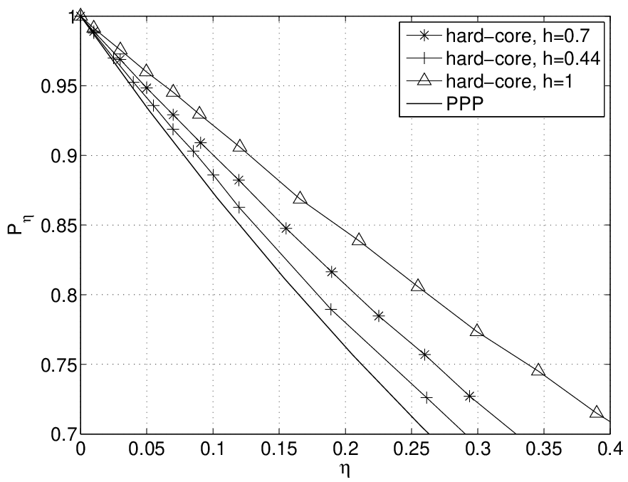
In this case, we start by generating a hard-core point process with intensity $\lambda=\lambda^{\prime}$ as given in (13) and then apply independent thinning with probability $\eta$ . In Figure 3 the success probability in a hard-core process network with ALOHA is shown. As proved in Theorem 2, we observe that $\mathsf{P}_{\eta}\sim 1-\gamma\eta$ , where $\gamma$ is given by (10). It can be observed that the outage probability improves as $h$ increases, as expected.

IV-B2 Poisson point process with CSMA

In this case, we start from a PPP with intensity $\lambda$ and adjust $h$ to thin the process to a Matern hard-core process of intensity $\lambda_{\mathrm{t}}=\lambda\eta$ , as given by (13) (where now $\lambda_{p}:=\lambda$ and the resulting $\lambda^{\prime}$ is the transmitter density $\lambda_{\mathrm{t}}$ ). Since we are interested in small $\eta$ or, equivalently, large $h$ , we obtain from (13) that $h\to\sqrt{1/(\pi\eta\lambda)}$ for large $h$ . So we have that the second-order product density $\rho^{(2)}(x)$ is zero for $\|x\|<\sqrt{1/(\pi\eta\lambda)}$ , and Condition (C.6) can be verified using (14), and hence the conditions of Corollary 1 are satisfied. Hence scaling the inhibition radius with $\eta^{-1/2}$ between the transmitters leads to $\kappa=\alpha/2$ , and the constant $\gamma$ is given by the following corollary.

Corollary 3.

When the transmitters are modeled as a Matern hard-core process and the MAC protocol decreases the density by increasing the inhibition radius $h$ such that $h=\Theta(\eta^{-1/2})$ , the spatial contention parameter $\gamma$ is given by

\gamma=\frac{\theta\lambda^{\alpha/2}\pi^{\alpha/2}2^{3-\alpha}}{\alpha-2}+4\theta\lambda\pi^{2}\int_{1/\sqrt{\lambda\pi}}^{2/\sqrt{\lambda\pi}}\frac{r^{1-\alpha}}{g(r)}\mathrm{d}r\,,

(16)

where

g(r)=2\pi-2\arccos\left(\frac{\sqrt{\lambda\pi}}{2}r\right)+\frac{r\sqrt{\lambda\pi}}{2}\sqrt{4-\pi\lambda r^{2}}.

Fig. 4 shows a simulation result for a PPP of intensity $\lambda=0.3$ , where hard-core thinning with varying radius $h$ is applied to model a CSMA-type MAC scheme, for $\alpha=4$ . It can be seen that the outage increases indeed only quadratically with $\eta$ and that the asymptotic expression provides a good approximation for practical ranges of $\eta$ . The spatial contention $\gamma$ can be obtained from (16); it is $\gamma\approx 1.95$ .

IV-C Poisson cluster processes (PCP)

A Poisson cluster process [11, 12] consists of the union of finite and independent daughter point processes (clusters) centered at parent points that form a PPP. The parent points themselves are not included in the process. Starting with a parent point process of density $\mu$ and deploying $c$ daughter points per parent on average, the resulting cluster process has a density of $\lambda=\mu c$ . The success probability in a Poisson cluster process, when the number of daughter points in each cluster is a Poisson random variable with mean $c$ is [8]

\mathsf{P}=\exp\left(-\mu\int_{\mathbb{R}^{2}}\Big[1-\exp(-c\beta(y))\Big]\mathrm{d}y\right)\\ \times\int_{\mathbb{R}^{2}}\exp(-c\beta(y))f(y)\mathrm{d}y,

(17)

where

\beta(y)=\int_{\mathbb{R}^{2}}\Delta(x-y)f(x)\mathrm{d}x,

and $f(x)$ is the density function of the cluster with $\int_{\mathbb{R}^{2}}f(x)\mathrm{d}x=1$ . In a Thomas cluster process each point is scattered using a symmetric normal distribution with variance $\sigma^{2}$ around the parent. So the density function $f(x)$ is given by

f(x)=\frac{1}{2\pi\sigma^{2}}\exp\left(-\frac{\|x\|^{2}}{2\sigma^{2}}\right).

The second-order product density for a Poisson cluster process is [11, 12, 6]

\rho^{(2)}(z)=\lambda^{2}\left[1+\frac{(f*f)(z)}{\mu}\right],

which, for a Thomas cluster process, evaluates to

\rho^{(2)}(x)=\lambda^{2}\left(1+\frac{1}{4\pi\sigma^{2}\mu}\exp\left(-\frac{\|x\|^{2}}{4\sigma^{2}}\right)\right).

(18)

IV-C1 ALOHA (daughter thinning)

For ALOHA, each node is retained with a probability $\eta$ and the resulting process is again a cluster process with daughter density $c\eta$ . Substituting $c\eta$ for $c$ in (17), it is easy to verify that $\kappa=1$ and $\gamma=\lambda^{-1}\int_{\mathbb{R}^{2}}\Delta(x)\rho^{(2)}(x)\mathrm{d}x$ , verifying Theorem 2. In Fig. 5, various configurations are shown with the corresponding analytical approximation obtained by the numerical computation of $\gamma$ using (18), and we observe a close match for small $\eta$ .

IV-C2 Highly clustered MAC (parent thinning)

A high clustered MAC can be obtained by thinning the parents (i.e., keeping or removing entire clusters) instead of the daughter points. This means that all the points induced by a parent point transmit with probability $\eta$ , and all of them stay quiet with probability $1-\eta$ . Such a MAC scheme causes highly clustered transmissions and high spatial contention. Even when the density of transmitting nodes gets very small, there are always nodes near the receiver that are transmitting. Such a MAC scheme violates Condition (C.1) in Theorem 1: The condition in this case is equivalent to

\mathcal{K}_{\eta}([0,1]^{2})=\int_{[0,1]^{2}}\frac{\rho^{(2)}(x)}{\lambda^{2}}\mathrm{d}x=\int_{[0,1]^{2}}\left[1+\frac{(f*f)(z)}{\eta\mu}\right]\mathrm{d}z,

and it follows that $\lim_{\eta\rightarrow 0}\mathcal{K}_{\eta}([0,1]^{2})\rightarrow\infty$ . From (17), it is easy to observe that

\mathsf{P}_{\eta}\leq\int_{\mathbb{R}^{2}}\exp(-c\beta(y))f(y)\mathrm{d}y<1,

i.e., the probability of success never reaches one because of the interference within the cluster. This is an example of an unreasonable MAC protocol.

IV-C3 Clustered MAC (parent and daughter thinning)

The ALOHA and highly clustered MAC schemes can be generalized as follows: For a MAC parameter $b\in[0,1]$ , first schedule entire clusters with probability $\eta^{1-b}$ (parent thinning) and then, within each cluster, each daughter may transmit with probability $\eta^{b}$ (daughter thinning). This results in a transmitter process $\Phi_{\eta}$ of intensity $\eta\lambda$ , as desired. It includes ALOHA as a special case for $b=1$ , and pure parent thinning for $b=0$ . For $b<1$ , the mean nearest-interferer distance scales more slowly than $\eta^{-1/2}$ , and we expect $\kappa<1$ . Indeed, it follows from (17) that $\kappa=b$ in this case. Fig. 6 shows a simulation result for $b=\kappa=1/2$ , which confirms the theoretically predicted sharp decay of the success probability near $\eta=0$ .

IV-D $d$ -dimensional TDMA networks

In a $d$ -dimensional lattice network³³ 3 with random translation and rotation for motion-invariance $\Phi=\mathbb{Z}^{d}$ , consider a TDMA MAC scheme, where every node transmits once every $m^{d}$ time slots so that only one node in a $d$ -dimensional hypercube of side length $m$ transmits. Since it takes $m^{d}$ time slots for this scheme to give each node one transmit opportunity, it is an $m^{d}$ -phase TDMA scheme, and the minimum distance between two transmitters is $m$ . In a regular single-sided one-dimensional $m$ -phase TDMA network with Rayleigh fading the success probability is bounded as [1, Eq. (31)]

e^{-\zeta(\alpha)\theta/m^{\alpha}}\leq{\mathsf{P}_{1/m}}\leq\frac{1}{1+\zeta(\alpha)\theta/m^{\alpha}},

(19)

where $\zeta$ is the Riemann Zeta function. The following theorem generalizes the bounds to lattices of dimension $d$ .

Theorem 4.

For $m^{d}$ -phase TDMA on $d$ -dimensional square lattice networks, the success probability is tightly bounded as

e^{-Z^{(d)}(\alpha)\theta\eta^{\alpha/d}}\leq\mathsf{P}_{\eta}\leq\frac{1}{1+Z^{(d)}(\alpha)\theta\eta^{\alpha/d}}\,,

(20)

where $\eta=m^{-d}$ and $Z^{(d)}$ is the Epstein Zeta function of order $d$ [15], defined (in its simplest form) as

Z^{(d)}(\alpha)\triangleq\sum_{x\in\mathbb{Z}^{d}\setminus\{o\}}\|x\|^{-\alpha}\,.

Proof:

Following the proof of [1, Prop. 3], for an $m^{d}$ -phase TDMA network

\mathsf{P}_{\eta}=\prod_{x\in\mathbb{Z}^{d}\setminus\{o\}}\frac{(m\|x\|)^{\alpha}/\theta}{1+(m\|x\|)^{\alpha}/\theta}\,,

(21)

Letting $\theta^{\prime}=\theta/m^{\alpha}$ , we obtain

\mathsf{P}_{\eta}^{-1}=\displaystyle\prod_{x\in\mathbb{Z}^{d}\setminus\{o\}}1+\theta^{\prime}/\|x\|^{\alpha}\,.

(22)

For the upper bound, ordering the terms according to the powers of $\theta^{\prime}$ yields

\mathsf{P}_{\eta}^{-1}=1+\theta^{\prime}Z^{(d)}(\alpha)+\theta^{\prime 2}(Z^{(d)}(\alpha)-1)+\ldots

Truncating this expansion at the second term, we obtain

\mathsf{P}_{\eta}\leq\frac{1}{1+Z^{(d)}(\alpha)\theta/m^{\alpha}}\,.

(23)

The lower bound in (20) is obtained by noting that $\eta=m^{-d}$ , taking the logarithm of (22) and using $\log(1+x)\leq x$ . ∎Fom the above theorem we observe that for a $d$ -dimensional TDMA network,

	$\displaystyle\gamma^{(d)}$	$\displaystyle=$	$\displaystyle Z^{(d)}(\alpha)\theta$		(24)
	$\displaystyle\kappa^{(d)}$	$\displaystyle=$	$\displaystyle\alpha/d,$		(25)

in agreement with Theorem 3 and Cor. 2. The conditions of Theorem 3 are satisfied since the support of $\rho^{(2)}(x)$ is zero for $\|x\|<\eta^{-1/d}$ . In one-dimension, $Z^{(1)}(\alpha)=2\zeta(\alpha)$ (which leads to (19) in the one-sided case). For TDMA in 2 and 3 dimensions [16],

	$\displaystyle\gamma^{(2)}=4\zeta(\alpha/2)\beta(\alpha/2)\theta$		(26)
	$\displaystyle\gamma^{(3)}\approx(4\upsilon(\alpha)\zeta(\alpha/2-1/2)\beta(\alpha/2-1/2)-$
	$\displaystyle\qquad\qquad 4\upsilon(\alpha)\zeta(\alpha-1)+8\zeta(\alpha/2)\beta(\alpha/2)-2\zeta(\alpha))\theta$

where $\beta$ is the Dirichlet beta function and

{\upsilon(\alpha)}=\frac{\sqrt{\pi}\Gamma(\alpha/2-1/2)}{\Gamma(\alpha/2)}.

In particular for $\alpha=4$ ,

	$\displaystyle\gamma^{(2)}$	$\displaystyle=\frac{2\pi^{2}}{3}G\theta\approx 6.03\,\theta$
	$\displaystyle\gamma^{(3)}$	$\displaystyle\approx\left(2\pi\zeta(3/2)\beta(3/2)-2\pi A+\frac{4\pi^{2}}{3}G-\frac{\pi^{4}}{45}\right)\theta$
		$\displaystyle\approx 16.53\,\theta\,.$

where $G\approx 0.916$ is Catalan’s constant, and $A=\zeta(3)\approx 1.202$ is Apéry’s constant. As expected, the spatial contention increases significantly from 2 to 3 dimensions.

Results on $Z^{(d)}(\alpha)$ for other special cases are presented in [16], a general method to compute $Z^{(d)}(\alpha)$ efficiently can be found in [17]. In Figure 7, the upper and lower bounds for the success probability are plotted for $d=1,2,3$ with $\alpha=4$ , $\theta=2$ .

IV-E Extensions

IV-E1 Different fading distributions

The results in this paper can be easily extended to any fading distribution between the typical receiver and the interferer’s as long as the distribution of the received power from the intended transmitter $\mathsf{S}$ is exponential. In this case only the definition of $\Delta(x)$ has to be modified (generalized) to

\Delta(x)=1-\mathcal{L}_{\mathsf{h}}(\theta\ell(x)),

and the rest of the derivations remain the same. Generalizing the results to non-exponential $\mathsf{S}$ would require techniques that are significantly different from the ones used here.

IV-E2 Swapping transmitter and receiver

Until now, we have analyzed the case where we declared the typical node at the origin to be the receiver under consideration. This way, the notation was simplified, and there was no need to add an additional receiver node. If instead, the typical transmitter is at the origin and its receiver is at a distance $R$ , such that $\ell(R)=1$ , then the results change as follows:

1.

ALOHA MAC protocol (Theorem 2): The new spatial contention parameter is

$\gamma_{\text{new}}=\lambda^{-1}\int_{\mathbb{R}^{2}}\rho^{(2)}(x)\Delta(x)\mathrm{d}x,$

where $\Delta(x)=\frac{1}{1+\theta^{-1}\ell(x-y)^{-1}},$ and $y=(\tilde{R},0)$ , where $\tilde{R}$ is the solution to $\ell(\|x\|)=1$ .
2.

Minimum-distance protocols (Theorem 3): The spatial contention parameter does not change and is given by (C.4).

In Figure 8, the success probability for ALOHA is plotted for the Matern hard-core process with the transmitter and the receiver exchanged, and we can observe that the outage is still linear asymptotically. For CSMA, see Figure 9 for an illustration of $\mathsf{P}_{\eta}$ and the asymptotic curve for the CSMA Matern process, when the transmitter and the receiver are swapped. As predicted, we observe that swapping the transmitter and the receiver has no effect on the asymptotic behavior.

IV-E3 Varying the link distance

Going back to the case where the typical receiver is at the origin, but its desired transmitter is at a general distance $R$ , then we have the following changes:

1.

ALOHA MAC protocol (Theorem 2): The spatial contention parameter is

$\gamma_{\text{new}}=\lambda^{-1}\int_{\mathbb{R}^{2}}\rho^{(2)}(x)\Delta(x)\mathrm{d}x,$

where

$\Delta(x)=\frac{1}{1+\theta^{-1}\ell(R)\ell(x)^{-1}}\,.$

Minimum-distance protocols (Theorem 3): We have

\gamma_{\text{new}}=\lim_{\eta\rightarrow 0}\theta\ell(R)^{-1}\lambda^{-1}\eta^{-\alpha/2-1}\int_{\mathbb{R}^{2}}\ell(x)\rho_{\eta}^{(2)}(x)\mathrm{d}x,

(27)

i.e., $\gamma$ gets multiplied by $\ell(R)^{-1}$ .

We observe that the spatial contention parameter $\gamma$ is scaled by $R^{2}$ in the case of a PPP with ALOHA, while for minimum-distance protocols (Matern hard-core processes) $\gamma$ gets scaled by $R^{\alpha}$ . In Figure 10, the success probability $\mathsf{P}_{s}$ of the CSMA protocol is plotted with respect to $R$ for $\alpha=4$ , and the $R^{4}$ dependency is confirmed. For other node distributions and MAC schemes, we presume that $\gamma$ scales like $R^{2\kappa}$ (for large $R$ ), since scaling the space $\mathbb{R}^{2}$ by $R$ changes the density by $R^{2}$ . The interference scaling exponent $\kappa$ does not change by swapping the typical transmitter and receiver, nor by changing the link distance.

Node distribution	MAC	Tuning parameter: $\eta$
PPP	ALOHA	Probability of transmission
Hard-core process	ALOHA	Probability of transmission
Hard-core process	CSMA	$\frac{1-\exp(-\lambda_{p}\pi h^{2})}{\lambda_{p}\pi h^{2}}$
PCP	ALOHA	Probability of transmission
$d$ -dim. lattice	$m^{d}$ TDMA	$m^{-d}$

TABLE I: This table summarizes the values of the tuning parameter

\eta

for different initial node distributions and MAC protocols. See Section IV for a detailed explanation of the point processes and MAC protocols under consideration.

V Conclusions

We have derived the asymptotics of the outage probability at low transmitter densities for a wide range of MAC protocols. The asymptotic results are of the form $\mathsf{P}_{\eta}\sim 1-\gamma\eta^{\kappa}$ , $\eta\rightarrow 0$ , where $\eta$ is the fraction of nodes selected to transmit by the MAC. The two parameters $\kappa$ and $\gamma$ are related to the network and to the MAC: $\gamma$ is the intrinsic spatial contention of the network introduced in [1], while $\kappa$ is the interference scaling exponent quantifying the coordination level achieved by the MAC, introduced in this paper. We studied $\mathsf{P}_{\eta}$ under the signal-to-interference ratio (SIR) model, for Rayleigh fading and with power-law path loss.

The numerical results indicate that for reasonable MAC schemes, the asymptotic result approximates the true success probability quite well for $\mathsf{P}_{\eta}>85\%$ . In terms of $\eta$ , this means that the approximation is good as long as $\eta<\eta_{\max}$ , where

{\eta_{\max}\approx\left(\frac{0.15}{\gamma}\right)^{1/\kappa}}\,.

So for small $\gamma$ and $\kappa=\alpha/2$ , the range of $\eta$ for which the approximation is good is fairly large.

Table II summarizes our findings and proposes a taxonomy for reasonable MAC schemes. ALOHA belongs to class R1 ( $\kappa=1$ ), irrespective of the underlying node distribution; hard-core MACs such as reasonable TDMA and CSMA are in class R3 ( $\kappa=\alpha/2$ ); while soft-core MACs which guarantee a nearest-transmitter scaling smaller than $\eta^{-1/2}$ are in class R2. Per Definition 1, the union of these three classes corresponds to the set of reasonable MAC schemes.

Class	Range of $\kappa$	Scaling	Remark
R1	$\kappa=1$	$\eta^{-1/2}$ on average	ALOHA
R2	$1\!<\!\kappa\!<\!\alpha/2$	$\eta^{-a}$ , $0<a<1/2$ , a.s.	soft-core MAC
R3	$\kappa=\alpha/2$	$\eta^{-1/2}$ a.s.	CSMA/TDMA

TABLE II: Summary of the results and proposed MAC taxonomy for reasonable MAC schemes. The scaling column indicates the nearest-neighbor distance scaling law as

\eta\to 0

Unreasonable MAC schemes are of less practical interest, but it is insightful to extend the taxonomy to these MAC schemes and give the ranges of the parameters $\kappa$ and $\gamma$ that pertain to them. The first class of unreasonable MAC schemes, denoted as U1, includes those MAC schemes for which the success probability goes to $1$ but $\kappa<1$ . This class is exemplified by the clustered MAC on a Poisson cluster process described in Subsection IV-C3. Next, the example of highly clustered MACs (parent thinning) in Subsection IV-C2 shows that there exist MAC schemes for which $\mathsf{P}_{0}=\lim_{\eta\to 0}\mathsf{P}_{\eta}<1$ . To incorporate such cases in our framework, we may generalize the asymptotic success probability expression to $\mathsf{P}_{\eta}\sim\mathsf{P}_{0}-\gamma\eta^{\kappa}$ for $\mathsf{P}_{0}\leq 1$ . This is Class U2. Lastly, there is an even more unreasonable class of MAC schemes, for which the success probability decreases as $\eta\to 0$ , which implies that $\gamma<0$ . The TDMA scheme in Fig. 2 is an example of such an extremely unreasonable MAC scheme, which constitutes Class U3. A summary of this taxonomy of unreasonable MAC schemes is given in Table III.

The different classes of MAC schemes can also be distinguished by the slope of the success probability at $\eta=0$ . A U1 MAC scheme has a slope of minus infinity, Class R1 has slope $-\gamma<0$ , and Classes R2 and R3 have slope 0. Class U2 also has zero slope but $\mathsf{P}_{0}<1$ , and U3 has a positive slope at $\eta=0$ , which is of course only possible if again $\mathsf{P}_{0}<1$ .

Another way of looking at the different classes of MACs is their behavior in terms of repulsion or attraction of transmitters. Class R1 (ALOHA) is neutral, it does not lead to repulsion or attraction, and whatever the underlying point process is, as $\eta\to 0$ , $\Phi_{\eta}$ approaches a PPP. Classes R2 and R3 induce repulsion between transmitters, which leads to the improved scaling behavior. Classes U1 to U3, on the other hand, induce clustering of transmitters.

While it is possible to achieve $\kappa=\alpha/2$ (class R3) for all point processes by choosing a good MAC scheme, it is also possible to end up in classes U1, U2, U3 for all point processes by choosing increasingly more unreasonable MACs. This indicates that for $\kappa$ (and the sign of $\gamma$ ) only the MAC scheme matters, not the properties of the underlying point process. As a consequence, at high SIR, a good outage performance can always be achieved, even if the point process exhibits strong clustering. Conversely, if the MAC scheme is chosen such that it favors transmissions by nearby nodes, the performance will be bad even if the points are arranged in a lattice.

Class	$\mathsf{P}_{0}$	Characteristic	Example
U1	$1$	$0\!<\!\kappa\!<\!1$	Cluster process in Fig. 6
U2	$<1$	$\gamma\geq 0$	Cluster process with $b=0$
U3	$<1$	$\gamma<0$	TDMA scheme in Fig. 2

TABLE III: Extension of the MAC taxonomy to unreasonable MAC schemes.

Our results also motivate the following conjecture: For all $0\leq\eta\leq 1$ , we conjecture that the success probability $\mathsf{P}_{\eta}$ of any network with a reasonable MAC is bounded by

1-\gamma\eta^{\kappa}\leq\mathsf{P}_{\eta}\leq\frac{1}{1+\gamma\eta^{\kappa}},

(28)

where $\gamma>0$ and $\kappa\geq 1$ are two unique parameters. The conjecture certainly holds in the case of ALOHA on the PPP (for all dimensions) per (6) and for (reasonable) TDMA on the lattice per (20).

When the transmitter and the receiver are swapped, this conjecture has to be modified to be valid for all $\eta$ . The conjecture as stated still holds for small $\eta$ , though.

Appendix

V-A Proof of Theorem 1

Proof:

Part 1 (lower bound): We first prove that $\kappa\geq 1$ . We will show that $1-\mathsf{P}_{\eta}=O(\eta)$ , which implies the result. From (4) we have

$\displaystyle\mathsf{P}_{\eta}$	$\displaystyle=$	$\displaystyle\mathbb{E}^{!o}\exp\left(-\theta\sum_{\mathsf{x}\in\Phi_{\eta}}\mathsf{h}_{\mathsf{x}}\ell(\mathsf{x})\right)$	(29)
	$\displaystyle\stackrel{{\scriptstyle(a)}}{{=}}$	$\displaystyle\mathbb{E}^{!o}\left[\prod_{\mathsf{x}\in\Phi_{\eta}}\mathbb{E}\exp(-\theta\mathsf{h}_{\mathsf{x}}\ell(\mathsf{x}))\right]$	(29)
	$\displaystyle\stackrel{{\scriptstyle(a)}}{{=}}$	$\displaystyle\mathbb{E}^{!o}\left[\prod_{\mathsf{x}\in\Phi_{\eta}}\frac{1}{1+\theta\ell(\mathsf{x})}\right]$	(30)
	$\displaystyle=$	$\displaystyle\mathbb{E}^{!o}\left[\prod_{\mathsf{x}\in\Phi_{\eta}}1-\Delta(\mathsf{x})\right]\,,$	(31)

where (a) is obtained by the independence of $\mathsf{h}_{\mathsf{x}}$ and (b) follows from the Laplace transform of an exponentially distributed random variable, and $\Delta(x)$ is given in (7). Using the inequality

\prod(1-y_{i})\geq 1-\sum y_{i},\quad y_{i}<1,

we obtain

\displaystyle\mathsf{P}_{\eta}

\displaystyle\geq

\displaystyle 1-\mathbb{E}^{!o}\sum_{\mathsf{x}\in\Phi_{\eta}}\Delta(\mathsf{x}).

(32)

Hence

	$\displaystyle\frac{1-\mathsf{P}_{\eta}}{\eta^{1-\epsilon}}$	$\displaystyle\leq$	$\displaystyle\eta^{\epsilon-1}\mathbb{E}^{!o}\sum_{\mathsf{x}\in\Phi_{\eta}}\Delta(\mathsf{x})$		(33)
		$\displaystyle=$	$\displaystyle\eta^{\epsilon}\lambda\int_{\mathbb{R}^{2}}(\lambda\eta)^{-2}\rho_{\eta}^{(2)}(x)\Delta(x)\mathrm{d}x,$		(33)

where $\rho^{(2)}_{\eta}(x)$ is the second-order product density of $\Phi_{\eta}$ . Eqn. (33) follows from the definitions of the second-order product density and the second-order reduced moment measure $\mathcal{K}_{\eta}(B)$ . Tesselating the plane by unit squares $S_{kj}=[k,\ k+1]\times[j,\ j+1]$ yields

\int_{\mathbb{R}^{2}}\lambda_{\mathrm{t}}^{-2}\rho_{\eta}^{(2)}(x)\Delta(x)\mathrm{d}x=\lambda_{\mathrm{t}}^{-2}\sum_{(k,j)\in\mathbb{Z}^{2}}\int_{S_{kj}}\rho_{\eta}^{(2)}(x)\Delta(x)\mathrm{d}x\,.

Let $\Delta_{kj}\triangleq\Delta(\min\{\|x\|,x\in S_{kj}\})$ . Since $\Delta(x)$ is a decreasing function of $\|x\|$ , we have

	$\displaystyle\int_{\mathbb{R}^{2}}\lambda_{\mathrm{t}}^{-2}\rho_{\eta}^{(2)}(x)\Delta(x)\mathrm{d}x$	$\displaystyle<\lambda_{\mathrm{t}}^{-2}\sum_{(k,j)\in\mathbb{Z}^{2}}\Delta_{kj}\int_{S_{kj}}\rho_{\eta}^{(2)}(x)\mathrm{d}x$
		$\displaystyle=\sum_{(k,j)\in\mathbb{Z}^{2}}\Delta_{kj}\mathcal{K}_{\eta}(S_{kj})$
		$\displaystyle\stackrel{{\scriptstyle(a)}}{{<}}C_{[0,1]^{2}}(\eta)\sum_{(k,j)\in\mathbb{Z}^{2}}\Delta_{kj}$
		$\displaystyle\stackrel{{\scriptstyle(b)}}{{<}}\infty,$

where $(a)$ follows from the transitive boundedness property of a PPD measure (see (8) for the definition of the constant $C_{[0,1]^{2}}(\eta)$ ), and $(b)$ follows from Condition (C.1) and since for $\alpha>2$ , $\sum_{(k,j)\in\mathbb{Z}^{2}}\Delta_{kj}<\infty$ . Hence it follows from (33) that

\lim_{\eta\rightarrow 0}\frac{1-\mathsf{P}_{\eta}}{\eta^{1-\epsilon}}=0\,,

which concludes the proof of the lower bound.
Part 2 (upper bound): Next we prove that $\kappa\leq\alpha/2$ . We will show that $1-\mathsf{P}_{\eta}=\Omega(\eta^{\alpha/2})$ , which implies the result. The success probability is

$\displaystyle\mathsf{P}_{\eta}$	$\displaystyle=$	$\displaystyle\mathbb{E}^{!o}\left[\prod_{\mathsf{x}\in\Phi_{\eta}}\frac{1}{1+\theta\ell(\mathsf{x})}\right]$
	$\displaystyle\leq$	$\displaystyle\mathbb{E}^{!o}\left[\prod_{\mathsf{x}\in\Phi_{\eta}\cap B(o,R\eta^{-1/2})}\frac{1}{1+\theta\ell(\mathsf{x})}\right]$
	$\displaystyle\leq$	$\displaystyle\mathbb{E}^{!o}\left[\frac{1}{1+\theta\ell(R\eta^{-1/2})}\right]^{\Phi_{\eta}(B(o,R\eta^{-1/2}))}$

As $\eta\rightarrow 0$ , $\ell(R\eta^{-1/2})\sim R^{-\alpha}\eta^{\alpha/2}$ , and using the identity $(1+x)^{-k}\sim 1-kx$ for small $x$ we obtain

$\displaystyle\lim_{\eta\rightarrow 0}\frac{1-\mathsf{P}_{\eta}}{\eta^{\alpha/2}}$	$\displaystyle\geq$	$\displaystyle\lim_{\eta\rightarrow 0}\mathbb{E}^{!o}[\Phi_{\eta}(B(o,R\eta^{-1/2}))]\theta R^{-\alpha}$
	$\displaystyle=$	$\displaystyle\lim_{\eta\rightarrow 0}\eta\lambda K_{\eta}(R\eta^{-1/2})\theta R^{-\alpha}$
	$\displaystyle\stackrel{{\scriptstyle(a)}}{{>}}$	$\displaystyle 0,$

where $(a)$ follows from (C.2). This concludes the proof of the upper bound on $\kappa$ . ∎

V-B Proof of Theorem 3

Proof:

From (11) we have

\mathsf{P}_{\eta}=\mathbb{E}^{!o}\prod_{\mathsf{x}\in\Phi_{\eta}}\frac{1}{1+\theta\ell(\mathsf{x})}.

It is easy to observe that

\mathbb{E}^{!o}\exp\Big(-\theta\sum_{\mathsf{x}\in\Phi_{\eta}}\ell(\mathsf{x})\Big)\leq\mathsf{P}_{\eta}\leq\mathbb{E}^{!o}\Big[\frac{1}{1+\theta\sum_{\mathsf{x}\in\Phi_{\eta}}\ell(\mathsf{x})}\Big]\,.

(34)

Let $\mathtt{I}_{\eta}=\sum_{\mathsf{x}\in\Phi_{\eta}}\ell(x)$ . By Jensen’s inequality we have

	$\displaystyle\mathsf{P}_{\eta}$	$\displaystyle\geq\exp\left(-\theta\,\mathbb{E}^{!o}\mathtt{I}_{\eta}\right)$
		$\displaystyle=\exp\left(-\theta\eta^{-1}\lambda^{-1}\int_{\mathbb{R}^{2}}\rho^{(2)}_{\eta}(x)\ell(x)\mathrm{d}x\right)\,.$

By Condition (C.4), we obtain

\lim_{\eta\rightarrow 0}\frac{1-\mathsf{P}_{\eta}}{\eta^{\alpha/2}}\leq\gamma.

To show the converse, we upper bound $\mathsf{P}_{\eta}$ as

	$\displaystyle\mathsf{P}_{\eta}$	$\displaystyle\leq$	$\displaystyle\mathbb{E}^{!o}\left[\frac{1}{1+\theta\mathtt{I}_{\eta}}\right]$		(35)
		$\displaystyle\leq$	$\displaystyle 1-\mathbb{E}^{!o}[\theta\mathtt{I}_{\eta}]+\mathbb{E}^{!o}[\theta^{2}\mathtt{I}_{\eta}^{2}]\,.$		(35)

It is easy to show that

	$\displaystyle\lambda\eta\mathbb{E}^{!o}[\mathtt{I}^{2}_{\eta}]$	$\displaystyle=\int_{\mathbb{R}^{2}}\ell^{2}(y)\rho^{(2)}_{\eta}(y)\mathrm{d}y$
		$\displaystyle+\int_{\mathbb{R}^{2}}\int_{\mathbb{R}^{2}}\ell(x)\ell(y)\rho^{(3)}(x,y)\mathrm{d}x\mathrm{d}y,$		(36)

which, combined with Conditions (C.5) and (C.6) implies $\mathbb{E}^{!o}[\mathtt{I}^{2}_{\eta}]\eta^{-\alpha/2}\rightarrow 0$ as $\eta\rightarrow 0$ . Hence it follows from (35) that

\lim_{\eta\rightarrow 0}\frac{1-\mathsf{P}_{\eta}}{\eta^{\alpha/2}}\geq\lim_{\eta\rightarrow 0}\theta\eta^{-\alpha/2}\mathbb{E}^{!o}[\mathtt{I}_{\eta}]=\gamma.

∎

V-C Proof of Corollary 1

Proof:

We show that in this case, Condition (C.4) holds. We focus on the singular path loss law $\ell(x)=\|x\|^{-\alpha}$ ; the other cases follow in a similar manner. Let $C_{1}\triangleq\gamma\lambda/\theta$ . We have

C_{1}=\int_{\mathbb{R}^{2}}\|y\|^{-\alpha}\rho_{\eta}^{(2)}(y\eta^{-1/2})\eta^{-2}\mathrm{d}y.

Since the support of $\rho^{(2)}_{\eta}(x)$ lies in $B(o,c\eta^{-1/2})^{c}\triangleq\mathbb{R}^{2}\setminus B(o,c\eta^{-1/2})$ we have

C_{1}=\int_{B(o,c\eta^{-1/2})^{c}}\|y\|^{-\alpha}\rho_{\eta}^{(2)}(y\eta^{-1/2})\eta^{-2}\mathrm{d}y.

Using the substitution $y\eta^{-1/2}\rightarrow x$ we obtain

C_{1}=\eta^{-1-\alpha/2}\int_{B(o,c\eta^{-1/2})^{c}}\|x\|^{-\alpha}\rho_{\eta}^{(2)}(x)\mathrm{d}x.

Letting $A_{k}=B(o,ck\eta^{-1/2})$ , we have

	$\displaystyle C_{1}$	$\displaystyle=\eta^{-1-\alpha/2}\sum_{m=1}^{\infty}\int_{A_{m+1}\setminus A_{m}}\\|x\\|^{-\alpha}\rho_{\eta}^{(2)}(x)\mathrm{d}x$
		$\displaystyle\leq\eta^{-1-\alpha/2}\sum_{m=1}^{\infty}(cm\eta^{-1/2})^{-\alpha}\int_{A_{m+1}\setminus A_{m}}\rho_{\eta}^{(2)}(x)\mathrm{d}x$
		$\displaystyle\stackrel{{\scriptstyle(a)}}{{=}}\eta\sum_{m=1}^{\infty}(cm)^{-\alpha}[K_{\eta}(\eta^{-1/2}(m+1))-K_{\eta}(\eta^{-1/2}m)],$

where $(a)$ follows from the identity $\int_{B(o,R)}\rho_{\eta}^{(2)}(x)\mathrm{d}x\equiv\lambda_{\mathrm{t}}^{2}K_{\eta}(R)$ . For large $R$ , we have $K(R)\sim\pi R^{2}$ , hence

K_{\eta}(\eta^{-1/2}(m+1))-K_{\eta}(\eta^{-1/2}m)\sim\pi\eta^{-1}(2m+1),

and thus $C_{1}<\infty$ for $\alpha>2$ . Using a similar method, Condition (C.5) can also be shown to hold in this case. So in CSMA networks whose inhibition radius scales as $\eta^{-1/2}$ , the conditions in Theorem 3 are satisfied and $\kappa=\alpha/2$ . ∎

References

[1] M. Haenggi, “Outage, Local Throughput, and Capacity of Random Wireless Networks,” IEEE Transactions on Wireless Communications, vol. 8, no. 8, pp. 4350–4359, Aug. 2009.
[2] F. Baccelli, B. Blaszczyszyn, and P. Mühlethaler, “An ALOHA Protocol for Multihop Mobile Wireless Networks,” IEEE Transactions on Information Theory, vol. 52, no. 2, pp. 421–436, Feb. 2006.
[3] S. Weber, X. Yang, J. G. Andrews, and G. de Veciana, “Transmission Capacity of Wireless Ad Hoc Networks with Outage Constraints,” IEEE Transactions on Information Theory, vol. 51, no. 12, pp. 4091–4102, Dec. 2005.
[4] M. Haenggi, J. G. Andrews, F. Baccelli, O. Dousse, and M. Franceschetti, “Stochastic Geometry and Random Graphs for the Analysis and Design of Wireless Networks,” IEEE Journal on Selected Areas in Communications, vol. 27, no. 7, pp. 1029–1046, Sep. 2009.
[5] A. Busson, G. Chelius, and J. M. Gorce, “Interference Modeling in CSMA Multi-Hop Wireless Networks,” INRIA, Tech. Rep. 6624, Feb. 2009.
[6] M. Haenggi and R. K. Ganti, “Interference in Large Wireless Networks,” Foundations and Trends in Networking, vol. 3, no. 2, pp. 127–248, 2008.
[7] F. Baccelli and B. Blaszczyszyn, “Stochastic Geometry and Wireless Networks: Applications,” Foundations and Trends in Networking, vol. 4, no. 1-2, pp. 1–312, 2009.
[8] R. K. Ganti and M. Haenggi, “Interference and Outage in Clustered Wireless Ad Hoc Networks,” IEEE Trans. on Information Theory, vol. 55, no. 9, pp. 4067–4086, Sep. 2009.
[9] M. Zorzi and S. Pupolin, “Optimum Transmission Ranges in Multihop Packet Radio Networks in the Presence of Fading,” IEEE Transactions on Communications, vol. 43, no. 7, pp. 2201–2205, Jul. 1995.
[10] M. Haenggi, “On Routing in Random Rayleigh Fading Networks,” IEEE Transactions on Wireless Communications, vol. 4, no. 4, pp. 1553–1562, Jul. 2005.
[11] D. Stoyan, W. S. Kendall, and J. Mecke, Stochastic Geometry and its Applications. John Wiley & Sons, 1995, 2nd Ed.
[12] D. J. Daley and D. Vere-Jones, An Introduction to the Theory of Point Processes: Volume II: General Theory and Structure, 2nd ed. Springer, 2007.
[13] O. Kallenberg, Random Measures, 4th ed. Akademie-Verlag, Berlin, 1986.
[14] K.-H. Hanisch, “Reduction of $n$ -th moment measures and the special case of the third moment measure of stationary and isotropic point processes,” Math. Operationsforsch. Statist. Ser. Statist., vol. 14, no. 3, pp. 421–435, 1983.
[15] P. Epstein, “Zur Theorie allgemeiner Zetafunktionen,” Mathematische Annalen, vol. 56, pp. 614–644, 1903.
[16] I. J. Zucker, “Exact results for some lattice sums in 2, 4, 6 and 8 dimensions,” J. Phys. A: Math. Gen, vol. 7, pp. 1568–1575, 1974.
[17] R. E. Crandall, “Fast evaluation of Epstein zeta functions,” Oct. 1998, available at http://people.reed.edu/~crandall/papers/epstein.pdf.

Outage Probability of General Ad Hoc Networks in the High-Reliability Regime

Abstract

Index Terms:

I Introduction

Definition 1 (Interference scaling exponent κ\kappa).

Definition 2 (Spatial contention parameter γ\gamma).

II System Model

III Outage Probability Scaling at Low Interferer Density

III-A General result

Theorem 1 (Bounds on the interference scaling exponent κ\kappa).

Definition 3.

III-B Achieving the boundary points κ=1\kappa=1 and κ=α/2\kappa=\alpha/2

Theorem 2 (Achieving κ=1\kappa=1).

Proof:

Theorem 3 (Achieving κ=α/2\kappa=\alpha/2).

Corollary 1 (CSMA).

Corollary 2 (dd-dimensional networks).

IV Examples and Simulation Results

IV-A Poisson point process (PPP) with ALOHA

IV-B Hard-core processes

IV-B1 Hard-core process with ALOHA

IV-B2 Poisson point process with CSMA

Corollary 3.

IV-C Poisson cluster processes (PCP)

IV-C1 ALOHA (daughter thinning)

IV-C2 Highly clustered MAC (parent thinning)

IV-C3 Clustered MAC (parent and daughter thinning)

IV-D dd-dimensional TDMA networks

Theorem 4.

Proof:

IV-E Extensions

IV-E1 Different fading distributions

IV-E2 Swapping transmitter and receiver

IV-E3 Varying the link distance

V Conclusions

Appendix

V-A Proof of Theorem 1

Proof:

V-B Proof of Theorem 3

Proof:

V-C Proof of Corollary 1

Proof:

References

Outage Probability of General Ad Hoc Networks
in the High-Reliability Regime

Definition 1 (Interference scaling exponent $\kappa$ ).

Definition 2 (Spatial contention parameter $\gamma$ ).

Theorem 1 (Bounds on the interference scaling exponent $\kappa$ ).

III-B Achieving the boundary points $\kappa=1$ and $\kappa=\alpha/2$

Theorem 2 (Achieving $\kappa=1$ ).

Theorem 3 (Achieving $\kappa=\alpha/2$ ).

Corollary 2 ( $d$ -dimensional networks).

IV-D $d$ -dimensional TDMA networks