In-medium effects in the holographic quark-gluon plasma
Abstract
In this article we use the gauge/gravity duality to investigate various properties of strongly coupled gauge theories, which we interpret as models for the quark-gluon plasma (QGP). In particular, we use variants of the D/D setup as an implementation of the top-down approach of connecting string theory with phenomenologically relevant gauge theories.
We focus on the effects of finite temperature and finite density on fundamental matter in the holographic quark-gluon plasma, which we model as the hypermultiplet in addition to the gauge multiplet of supersymmetric Yang-Mills theory.
We use a setup in which we can describe the holographic plasma at finite temperature and either baryon or isospin density and investigate the properties of the system from three different viewpoints.
(i) We study meson spectra. Our observations at finite temperature and particle density are in qualitative agreement with phenomenological models and experimental observations. They agree with previous publications in the according limits.
(ii) We study the temperature and density dependence of transport properties of fundamental matter in the QGP. In particular, we obtain diffusion coefficients. Furthermore, in a kinetic model we estimate the effects of the coupling strength on meson diffusion and therewith equilibration processes in the QGP.
(iii) We observe the effects of finite temperature and density on the phase structure of fundamental matter in the holographic QGP. We trace out the phase transition lines of different phases in the phase diagram.
1 Introduction
The entire content of matter and radiation in the universe is a manifestation of the energy unleashed in some unknown process which we commonly refer to as the big bang. This event is thought of as the moment of the creation of matter, space and time — the universe. From that moment on energy existed in various manifestations. At an order of magnitude of seconds after the big bang, quarks formed. Today we experimentally detect these particles together with leptons and the force mediating gauge bosons as the fundamental constituents of all visible matter. The interaction of these particles is described incredibly accurately within two different theories. Processes taking place at energy levels below the TeV scale involving electromagnetic, weak and strong interaction are described accurately by the standard model of particle physics, although the strong force is hard to exploit theoretically at low energies for mathematical reasons. The fourth of the known forces, gravity, is described within the separate framework of general relativity.
While many aspects of the particles that make up our world are well understood, others remain a mystery. Among the latter is the behavior of matter under conditions that must have existed shortly after the big bang. The earliest period of the universe that can either be described by theoretical models and numerical simulations or probed by experiments is ranging from about seconds after the big bang when quarks and gluons emerged until approximately seconds after the big bang when hadronization of quarks set in. During this early phase matter existed in conditions of extremely high density and temperature. Under these conditions quarks are not confined and do not form hadrons. Instead they are moving independently and interact with each other predominantly via the exchange of gluons, which mediate the force of strong interactions. As typical for plasmas, the freely moving quarks allow for (color) charge screening. Matter in this phase is therefore referred to as the quark-gluon plasma (QGP).
From the beginning on, the universe expanded and cooled down. After seconds at a critical value of the temperature of approximately 160–190 MeV the energy dependent coupling constant of the strong force rose to a value that let confinement set in. Eventually quarks combined to bound states and formed the hadronic matter that is now composing the galaxies visible in the universe. Only very particular regions of the present universe come into consideration for providing conditions extreme enough to contain matter in the phase of the quark-gluon plasma. Such barren places are the cores of neutron stars. These are remnants of supernova explosions of stars of about 20–30 solar masses. Due to the extremely high gravitational pressure, the hadronic matter existing on the planets surface in deeper layers is squeezed together to such an extent that electrons and protons combine to neutrons (thereby emitting neutrinos). From the surface towards the core of these objects the pressure increases. In the inner layers even neutrons are not stable anymore. Instead the quarks and gluons may interact individually to appear as the QGP. Other temporary habitats of the quark-gluon plasma seem to exist on earth: The experiments conducted at heavy ion colliders are dedicated to monitor the processes occurring at collisions of heavy nuclei at energies high enough to produce a fireball of extremely hot and dense matter. Such experiments are hosted at the Super Proton Synchrotron (SPS), the Relativistic Heavy Ion Collider (RHIC) accelerating gold nuclei, and in future also the Large Hadron Collider (LHC) which can be used to accelerate lead nuclei, as well as future SIS experiments at the Facility for Antiproton and Ion Research (FAIR). The state of matter observed at RHIC is a strongly coupled system composed of deconfined quarks and gluons, the strongly coupled quark-gluon plasma (sQGP).
To get an impression of the processes occurring during the first moments after the creation of the universe — including the interactions of quarks and gluons which lead to the genesis of the hadronic matter that composes our world — it is necessary to understand the properties of the quark-gluon plasma. This will eventually allow for deeper insight into the process of hadronization and the phase transition from the quark-gluon plasma to the hadronic phase. Further knowledge about the nature of matter may also allow for progress in finding the answer to questions about the nature of dark matter and dark energy, the majority of the energy content of our universe — by far greater than the contributions visible matter can account for.
Still a manageable theoretical description of the interaction of quarks and gluons in the strongly coupled systems observed at experiments is not straightforward, although the standard model contains a theory of quarks and gluons, known as quantum chromodynamics (QCD). It is the strong coupling that impedes the solution of the equations of motion of QCD at low energies. Analytical answers from QCD are obtained from perturbation expansions in the coupling constant, which do not converge at strong coupling. Therefore today there is no analytic description of the formation of bound states of quarks or the interaction of quarks and gluons in the sQGP from first principles. One successful alternative to obtain results at strong coupling is lattice gauge theory, which tries to simulate the dynamics of QCD numerically on a number of discrete points in spacetime. While this approach gave answers to numerous questions, by nature it cannot produce analytical results which would lead to conceptual insights. It moreover approximates spacetime as a coarse grid and so far has to incorporate some simplifications of QCD.
A completely different approach to the quark-gluon plasma can be pursued from a point of view that also motivates the work presented in this work. A possible alternative to the description of strongly coupled quarks and gluons may be given in terms of string theory. This theory assumes strings to be the fundamental degrees of freedom, from which all matter is composed. The different elementary particles we know are thought to arise as the different oscillation modes of the strings. Initially, around 1970, it aimed to explain the relation between spin and mass of the resonances found in then performed collision experiments, , with known as the “Regge slope”. The idea was to describe the force between quarks as if a string of tension holds the particles together. Despite modeling the Regge behavior, the theory failed to describe the observed cross sections correctly and was successfully displaced by QCD wherever applicable. Nevertheless, the understanding and interpretation of string theory evolved to a great extent, especially the possibility to describe quantized gravity attracted interest. Today it is the most promising candidate for a unified description of all known forces of nature within one single theory. In this sense it can be thought of as a generalization of the successful standard model by including a description of gravity. The world of strings appears as a stunningly complex system that may give answers to such fundamental questions as the origin of the number of spacetime dimensions we live in, and allow for a formulation of quantum gravity. Still much of the theory has to be understood and almost no predictions lie within the reach of experimental verification.
However, during the past dozen years evidence mounted that indeed there are connections between string theory and gauge theories, like QCD. In the mid 1990s, during the so called second string theory revolution, it was discovered that string theory not only features strings as degrees of freedom. In addition, there are higher dimensional objects, called branes as an allusion to membranes. Branes and strings interact with each other. In this way branes influence the degrees of freedom introduced by the string oscillations. As the understanding of string theory grew, it was discovered that certain limits of string theory contain the degrees of freedom of particular non-Abelian gauge theories. These insights heralded a new era of applications of string theory to problems in gauge theory. It began in 1997 with Juan Maldacena’s discovery of analogies between the classical limit of so called type IIB string theory, including branes, and the supersymmetric Yang-Mills quantum gauge field theory. It is possible to establish a one to one mapping between the degrees of freedom of both theories. Maldacena therefore speculated that both of them are different descriptions of the same physical reality. The formulation of this conjecture is known as the /CFT correspondence [6]. As we will discuss later, this correspondence between type IIB string theory in Anti-de Sitter space () and the supersymmetric non-Abelian conformal field theory (CFT) is especially suitable to describe the strongly coupled regime of gauge theories. An astonishing feature of the /CFT correspondence is that it conjectures the equivalence of a classical theory of gravity and a quantum field theory. In some aspects this field theory resembles the properties of QCD. Moreover, it relates the strongly coupled regime of the quantum field theory to the weakly coupled regime of the related gravity theory. One therefore can obtain strong coupling results of field theory processes by means of well established perturbative methods on the gravity side. Finally, the /CFT correspondence allows to interpret the quantum field theory to be the four dimensional representation of processes in string theory, which is defined in ten spacetime dimensions. Because of these properties the correspondence is more generally also referred to as gauge/gravity duality and is said to realize the holographic principle. So far there is no mathematically rigorous proof for the correspondence to hold. Nevertheless, in all cases that allowed for a direct comparison of results from both theories, perfect matching was found.
The /CFT correspondence is considered as one of the most important achievements in theoretical physics of the last decades. However, by now the string theory limit which exactly corresponds to QCD is not known. Albeit the direct way ahead towards a comprehensive analytical description of strongly coupled QCD is not foreseeable, numerous cornerstones where already passed and some junctions and connections to the related physical disciplines where found. Examples are deeper insights into the connection of black hole physics to thermodynamics, the relation to finite temperature physics, and the discovery of quantities like the famous ratio of shear viscosity to entropy density that are universal for large classes of theories. The motivation to use the /CFT correspondence to explore the strongly coupled quark-gluon plasma therefore is twofold. On the one hand side there is the attempt to provide a description of strongly coupled quarks and gluons as a supplement to QCD. In this way string theory might contribute to further understanding of gauge theories. On the other hand a phenomenologically relevant application of string theory can be used as a benchmark to evaluate the capabilities of string theory in describing nature. In this way string theory might benefit from the exploration of new regimes of QCD, so far described predominantly by quantum field and lattice gauge theories. The ability to produce the sQGP in collision experiments for the first time may allow to check predictions from string theory. There is well-founded hope that the quark-gluon plasma can provide a link between string theory and experiment.
We will make use of the /CFT correspondence to investigate strongly coupled systems. The models we use for this purpose will be various modifications of the gauge/gravity duality that allow for the description of quantum field theories that feature certain aspects known from QCD. Which aspects and which parameter regions we can cover with this approach will be pointed out in the introductory section on /CFT and in those sections where we introduce the models. It is interesting in its own to see how far the correspondence may be extended and which facets of quarks and gluons can be modeled at all. However, it is even more fascinating to see that already today some properties of phenomenological relevance can be captured by a so called holographic description of the sQGP via the /CFT correspondence. Such results allow for comparison with lattice gauge theory and effective field theories. A vast number of attempts to apply the correspondence to the dynamics of quarks and gluons has been under investigation during the past years. The questions pursued in this work are the following.
- •
Can quarks and gluons combine to form hadrons inside the quark-gluon plasma? How does the spectrum of bound states of quarks, esp. of mesons, look like inside the sQGP?
- •
How do these spectra and the lifetime of mesons depend on temperature and quark density?
- •
How do quarks and their bound states move through the plasma?
- •
What effects has the strong coupling?
The answers we obtain are by part of qualitative nature, or can be expected to receive corrections, which can be calculated as soon as progress in the field allows to relax some limiting assumptions. Nevertheless, it is amazing to see that the gauge/gravity duality can give answers to these questions in terms of a minimal number of input parameters. We do not follow the so called “bottom-up” approach, also known as /QCD. There the goal would be to find gravity duals to phenomenological gauge theories which incorporate certain desired aspects of QCD. Instead we pursue the “top-down” approach. This means that we are aware of the fact that the /CFT correspondence is a phenomenon discovered in string theory. We try to construct models which are consistent solutions of string theory and observe the consequences on the gauge theory side. From this point of view, the results obtained by means of the /CFT correspondence can be interpreted as a sign of the predictive power of string theory.
This article is organized as follows. Section 2 gives a brief introduction to the gauge/gravity duality, the extensions which are of relevance for the derivation of our results, and a short discussion of the application to QCD and the quark-gluon plasma. However, we will not try to give an introduction neither to string theory nor to quantum field theory, supersymmetry or general relativity. Nevertheless, these theories are the basis of this work. Especially string theory is on the one hand the basis of this work, on the other hand too rich to provide a broad background in detail here. Therefore, we will provide the necessary theoretical arguments and details wherever needed in a hopefully adequate manner. The remaining sections deal with the answers of the questions mentioned above. Each of them contains a brief introductory section and one or more technical sections which lead to results that will be discussed at the end of each section. In particular, section 3 deals with meson spectra at finite temperature and particle density, and discusses the influence of these parameters on the spectra. In section 4 transport coefficients of quarks and mesons in the plasma are calculated. Comparison with weak coupling results enables us to estimate the effects of strong coupling. In section 5 we examine the lifetime and stability of mesons at different temperatures and particle densities and in this way get new insights into the structure of the phase diagram of the dual field theory. A summary and discussion of the results is finally given in section 6. Appendices clarify conventions and notational issues and present some calculations in a more detailed form than the main text allows for.
2 The AdS/CFT correspondence and extensions
Conventional holograms are able to encode truly three-dimensional information on a two-dimensional surface. Analogously, in particle physics and quantum gravity, the equivalence of information contained in a theory defined in some lower dimensional space and a different theory on a higher dimensional domain, is referred to as the holographic principle. One of the first observations of such kind of holography was the discovery that the information captured inside the horizon radius of a black hole, i. e. the entropy given by the number of possible microstates, can be described in terms of the horizon surface area alone [7]. This observation suggests the existence of a holographic realization of quantum gravity.
Another observation of a holographically realized connection between gravitational physics and quantum mechanics was made by Juan Maldacena at the end of the so-called second string theory revolution. He then conjectured the equivalence of a supergravity theory in Anti-de Sitter spacetime () and a certain type of conformal field theory (CFT) [6]. This discovery triggered an enormous amount of efforts to establish the long sought connection between quantum gauge field theories and gravity, which did not abate so far. The fact that the theory on the side of the correspondence can be expressed as a low energy limit of string theory, which naturally incorporates gravity, is widely interpreted as a support of the claim of string theory to offer a formalism which allows for a unified description of all known fundamental forces of nature.
In this section we briefly review the Maldacena conjecture and some of the extensions invented during the last decade. Instead of giving an exhaustive review, we merely draw a hopefully concise and consistent sketch of the whole picture. In doing so we emphasize those features of the correspondence that are most important for the developments in the subsequent sections. Classical reviews which deal with the subject in depth are refs. [8, 9]. For the sake of clarity, we restrict explicit calculations to a minimum here.
2.1 The original AdS/CFT correspondence
The /CFT correspondence as it was formulated by Maldacena in 1997 relates two particular theories which we introduce subsequently. Afterwards we rephrase the conjecture of Maldacena, before we comment on the relaxation of the underlying assumptions, other generalizations and the applicability to QCD and the quark-gluon plasma in the following sections.
2.1.1 Super-Yang-Mills theory
One of the two theories related by the /CFT correspondence is super-Yang-Mills theory in four spacetime dimensions of Minkowski topology. It is a supersymmetric quantum field theory with R-symmetry, which rotates the four supercharges into each other. All fields are arranged in one supersymmetry multiplet. The on-shell field content is given by six real spacetime scalars with , one spacetime vector field and four two component spin left Weyl fermions with . Under R-symmetry transformations the six scalars transform as an antisymmetric of rank two. The Weyl fermions represent a and the vector field is a singlet.
With respect to gauge symmetries, all the fields constitute one single multiplet, called the gauge multiplet. They transform under the adjoint representation of the gauge symmetry group , where the integer is left as a parameter for now. Later we will interpret it as the number of color degrees of freedom.
The according gauge indices labeling the elements of the gauge symmetry generators with are suppressed in our notation, e. g. the notation for a spacetime scalar is the short form of where as a matrix has elements labeled by . One would write out the elements of as , where labels the index which transforms under the of the R-symmetry and are the indices transforming under gauge symmetries. We label spacetime directions by and . With this convention and the field strength tensor the unique Lagrangian [9] reads as
| (2.1) | ||||
where the trace is performed over the suppressed gauge indices and is the gauge covariant derivative. The symbol denotes the real valued instanton angle, the and are related to the structure constants of the R-symmetry group, and there is one dimensionless coupling constant in this Lagrangian. The energy dimensions of the operators and constants are given by
| (2.2) |
so the action is scale invariant. In fact theory is invariant under transformations generated by the conformal symmetry group composed by Poincaré transformations, scaling and so-called superconformal transformations as well as under the above mentioned R-symmetry group . These transformations compose the global symmetry group denoted by . Note that these symmetries are realized also in the quantized theory and not broken by anomalies. Moreover, the Lagrangian of super-Yang-Mills theory is unique. In contrast to other supersymmetric theories, which allow for different choices of the potential for the superfields, the form of the action is completely determined by the demand for renormalizability.
There even is a further symmetry. With respect to the complex combination of the coupling and the instanton angle given by
| (2.3) |
the action is invariant under . Generalizing this symmetry, the Montonen-Olive conjecture states that the theory is invariant under transformations acting on the complex coupling , this symmetry is denoted as S-duality. It includes a transformation which indicates that the theory describes a duality between strongly and weakly coupled regimes. We will not make use of this duality, though.
The large limit and the connection to string theory
The super Yang-Mills theory introduced here is strongly related to string theory, which becomes visible in the limit of asymptotically many colors, , while the effective coupling is kept fix. This is the so-called ’t Hooft limit [10]. The motivation to consider the large limit is to find a parameter which allows for perturbative calculations in strongly coupled gauge theories, namely 1/N. To illustrate this in a simplified way for the theory given by (2.1), we note that one can schematically write the interaction terms of this Lagrangian as
| (2.4) |
where are any of the bosonic fields or (and the fermions are related to them by supersymmetry). Note that the three-point vertices are proportional to while the four-point vertices are proportional to . After the introduction of the Lagrangian acquires the form
| (2.5) |
Remember that all fields of SYM theory transform in the adjoint representation of the gauge group . So can be written in a matrix notation, where the elements of the matrix are denoted by , with transforming in the fundamental and antifundamental representation, respectively. In a Feynman diagram a propagator for some particle then corresponds to a double line, with one line corresponding to the upper and one to the lower index , of the gauge group, see figure 2.1.
In this double line notation we can now order diagrams in an expansion parametrized by to see that the contributions to gauge invariant processes may be ordered according to the Euler characteristic of the Feynman diagram, i. e. they are ordered according to topology of the diagram. As an example consider the diagrams in fig. 2.1. For the amplitude corresponding to some Feynman diagram, a propagator introduces a factor of while the above Lagrangian (2.5) shows that vertices pick up a factor of . From the double line notation it is clear that each closed line therein represents a loop which introduces a factor . Moreover, think of the diagrams as describing polyhedrons which are characterized by vertices, edges (propagators), and faces which are the regions separated by the edges. We observe that the factors of for a diagram with vertices, edges and faces (i. e. loops of lines in the double line diagrams) appear in powers of
| (2.6) |
The number is the Euler character of the polyhedron described by a Feynman diagram. The genus of the corresponding Riemann surface is given by . From this dependence on we see that diagrams with smallest , i. e. planar diagrams with , contribute with highest order, while diagrams with topologies of higher genus are suppressed by factors of relative to the planar ones. In this way any process in the field theory can be decomposed into diagrams ordered by their genus in the double line notation. The amplitude of a given process may then be obtained by a sum of the contributions from all relevant Feynman diagrams,
| (2.7) |
This type of expansion is exactly the same as the one obtained by performing an expansion of diagrams describing the interaction of closed oriented strings, the type II string theories, upon recognizing the parameter as being proportional to , the string coupling constant [8]. The hope is, that the topologies of Feynman diagrams reflect the contribution of the string theory diagrams with the same topology. From the standard examples shown in figure 2.1 we see that the genus represents the number of loops in the associated string theory diagram.

The large limit corresponds to weakly coupled string theory, as . In this limit we only have to consider the leading diagrams with genus . These are the gauge theory processes described by planar diagrams, corresponding to tree level diagrams in string theory.
These arguments are of heuristic nature. For instance, there are effects like instantons in a gauge theory, which can not be treated in a expansion. Such effects therefore should match the according non-perturbative effects in string theory.
2.1.2 Type IIB supergravity
The preceding section introduced the quantum field theory, which represents one of the two theories connected by the /CFT correspondence. The second theory is type IIB supergravity. Supergravity theories are supersymmetric gauge field theories containing a spin field identified with the graviton, the quantum field of gravitation. Supergravity thereby is an attempt to combine supersymmetric field theory with general relativity.
Even though Supergravity is an interesting field to study on its own right, it can be embedded in a larger and more general framework. In fact supergravity is a certain limit of string theory. A brief comment on this perception will follow below. As string theory revealed that a consistent description of the forces and matter of nature requires ten spacetime dimensions, we will be interested in a formulation of supergravity in ten-dimensional backgrounds. There are different supergravity theories in ten spacetime dimensions, which can be constructed from compactifications of a unique causal unitary -dimensional supergravity theory [9].
The one formulation we will make use of throughout this monograph, and which is the one most intimately connected with the /CFT correspondence is the so-called type IIB supergravity in ten spacetime dimensions. This theory is a supersymmetric theory with a field content given by the bosonic fields (symmetric rank , the metric), (scalar, axion), (scalar, dilaton), (rank antisymmetric, Kalb-Ramond field), (rank antisymmetric), (self dual rank antisymmetric). The fermions of the theory satisfy Majorana-Weyl conditions and are given by two (, spin gravitinos of same chirality) and two fields (, spin dilatinos of same chirality, which is opposite to the chirality of the gravitinos). This theory is chiral in the sense that it is parity violating [9].
The action of type IIB supergravity may be written down in terms of the field strengths
| (2.8) | ||||||
| (2.9) | ||||||
| (2.10) |
and then reads
| (2.11) | ||||
where is the Newton constant and is the Ricci scalar. Additionally, at the level of the equations of motion one has to impose the self-duality constraint
| (2.12) |
Type IIB supergravity as a string theory limit
Starting from the Polyakov action to describe string world sheets, tachyonic string modes were discovered in the derived spectrum. These tachyons indicate an instability of the theory. To arrive at a stable and causal theory, one should remove these tachyonic excitations from the spectrum. To do so, one may modify the Polyakov action by introducing supersymmetry, and truncate the spectrum of physical states in a consistent way, a procedure called GSO-Projection (after the inventors Gliozzi, Scherk and Olive). This projection exactly leaves a spacetime supersymmetric spectrum.
This procedure not only removes the tachyonic ground state from the closed string spectrum but additionally demands a number of spacetime dimensions to preserve causality. The lowest remaining modes after the GSO projection represent the ground state of the remaining theory. For instance, in the Neveu-Schwarz sector of the string excitations this ground state happens to be described by massless excitations of strings. The so-called level matching condition demands this state to be generated from a vacuum by the action of two creation operators, a left- and a right-moving one, . These excitations may be described by a tensor valued field with components . This field in turn decomposes into a symmetric part with components (describing the degrees of freedom of the graviton), antisymmetric components (the -field) and the scalar (the dilaton) that determines the trace of .
Computing the masses of string excitations generated by more than two creation operators acting on the vacuum, unveils that these excitations describe fields which represent particles of finite positive mass proportional to . In a low energy theory compared to the energy scale of inverse string length, or equivalently on length scales that do not resolve the stringy nature of the fundamental theory one may approximate the strings by pointlike particles, effectively described as . In this limit, however, all massive modes gain infinite masses and will not effect the low energy dynamics. The low energy theory may therefore only contain particles described by the massless supersymmetry multiplet to which the fields , and belong. The action remaining for these fields exactly describes the supergravity action. We are interested in the sector of closed string excitations with same chirality for the left and right moving excitations, which is called type IIB string theory and leads to type IIB supergravity in the low energy limit.
In the action (2.11) above, the fields , and can be found in the first line, they originate from the Neveu-Schwarz sector (NS-NS) of the string theory fields, while the second and third lines contain the Ramond sector (R-R) contributions.
Extremal p-brane solutions and D-branes
Solutions to the supergravity equations of motion with non-trivial charges of -forms are called p-branes. These solutions exhibit Poincaré-invariance in dimensions, their name thus stems from the number of spatial dimensions included in this symmetry group. In this sense these solutions are higher dimensional generalizations of membranes, which one would denote as -branes in this context.
Note that the flux of the field strength through some surface is conserved since , as is an exact and thus closed form. Moreover, the electric coupling of the -form to the -brane with worldvolume of spacetime dimension can be described by the diffeomorphism invariant action
| (2.13) |
The proportionality constant denotes the tension of the -brane. It has the interpretation of the energy or mass per unit area of the worldvolume,
| (2.14) |
In type IIB supergravity, there are -forms, -forms and -forms, allowing for the following -brane solutions. The -forms allow for -brane solutions, so-called D-instantons. Then there are -branes, charged under and thus coupling to the according solutions of the -field. The two dimensional -branes are identified with the worldsheet of the fundamental strings of the underlying string theory. They are called F-strings. The -branes which couple to the field are called D-strings, and the -brane solutions according to the field are called D-branes.
The magnetic analogon to the electric couplings are given by the Hodge dual field strengths. The magnetic dual field strength to in a ten-dimensional background, is the -form , which has a -form field as its potential. This in turn couples to a -brane. In this way the type IIB field strengths and allow for magnetic couplings to D-branes and D-branes.
The naming of branes as D-branes we just saw, arises from string theory. As we can see, the D-branes are coupling to fields in the Ramond sector. The letter D is short for the Dirichlet boundary conditions such a brane imposes on the dynamics of the endpoints of open strings. Namely, in string theory D-branes are identified with the surfaces on which open strings end [11, 12]. The endpoints of these strings then have a well defined position in the direction perpendicular to the brane, namely the position of the brane. Such a specification of a certain value for a actually dynamical quantity is known as the imposition of Dirichlet boundary conditions. It is believed that the -brane solutions in the supergravity limit of string theory may be identified with D-branes in full string theory.
The fact that -branes are -dimensional Poincaré invariant imposes restrictions on the metric. For instance, some -dimensional spacetime which supports a -brane will include a Poincaré invariant subspace with symmetry group . Additionally, one can always find solutions which are maximally rotationally invariant in the -dimensional space transverse to the brane. Thus, in particular a ten-dimensional spacetime supporting D-branes has an isometry group of .
Analog to Reissner-Nordström black holes in general relativity, the possible solutions of supergravity backgrounds can be parametrized by the mass of the -brane solution and its RR charge , which are functions of two parameters , which can be interpreted as horizons of the solution. The case exhibits a naked singularity and is therefore regarded as unphysical. In the limit of the brane is said to be an extremal -brane, while it is a non-extremal black brane for , with an event horizon. For details refer to ref. [8]. We restrict our attention to the case of extremal -branes.
The most general form of an extremal -brane metric can be written in terms of a function as [9]
| (2.15) |
Here, the coordinates of the vector parametrize the space transverse to the brane, and is the -dimensional Minkowski metric.
Supported by the insight that D-branes are dynamical objects of the theory [11], one can adopt the point of view that the above geometry is generated by a stack of branes placed in an initially flat -dimensional Minkowski spacetime at a positions , with . Asymptotically far away from the stack one can therefore expect the whole spacetime to become flat again. String theory calculations then restrict the function to
| (2.16) |
where is the string coupling constant and parametrizes the string tension.
Of special interest for this article are D-branes and D-branes. For the introduction of the /CFT correspondence, it is useful to look at D-branes first. D-branes will become an important ingredient for generalizations of the correspondence.
D-branes and Anti-de Sitter space
There are several aspects which make D-branes especially interesting. First of all, D-branes by definition introduce four-dimensional Poincaré symmetry, the resulting ten-dimensional geometry for is regular. Moreover, the solution for the axion and dilaton fields ( with and in (2.11)) can be shown to be constants. In addition, the field strength is self-dual. For our considerations the metric will be a central quantity. Especially the case of coincident D-branes located at a position in a spacetime of dimension will be important. From (2.16) we see that the function in this case is given by
| (2.17) |
We introduce the quantity simply as an abbreviation,
| (2.18) |
However, a few lines below we will see that this parameter has a crucial geometric interpretation. With we write as
| (2.19) |
By a coordinate shift we may always denote the position as the origin of the coordinates and set it to zero. The distance from the brane will be denoted by . The metric (2.15) generated by a stack of D-branes therefore may be written as
| (2.20) |
Far away from the stack of branes, at large , where the influence of the branes on spacetime will not be sensible, the metric is asymptotically flat ten-dimensional Minkowski spacetime. However, in the limit of the metric appears to be singular. This limit is therefore known as the near horizon limit. In fact spacetime is not singular in this limit but develops constant (negative) curvature. Because space is flat at large , but has constant curvature at this limit is also referred to as the throat region. In the near horizon limit at small the metric asymptotically becomes
| (2.21) |
This is the product space , where the first two terms describe what is known as five-dimensional Anti-de Sitter space, or for short. The parameter is called the radius of space. The last term represents the familiar five-dimensional sphere, of radius as well. The geometry of Anti-de Sitter space is crucial for the gauge/gravity duality. To discuss some properties we introduce the coordinate and write the metric as
| (2.22) |
The metric (2.22) can be derived as the induced metric of a five-dimensional hypersurface which is embedded into a six-dimensional spacetime with metric
| (2.23) |
where the parametrize the six-dimensional space and the choice of the ambiguous sign depends on whether we aim for a metric on with Euclidean or Minkowski signature. Originally, the /CFT correspondence was conjectured for Euclidean signature. The hypersurface which defines obeys
| (2.24) |
We now parametrize this surface with so-called Poincaré coordinates and with , such that with the sign corresponding to the one in (2.23) and
| (2.25) | ||||
The hypersurface parametrized by and the fulfills (2.24) and therefore represents . It has the induced metric
| (2.26) |
which appears as the first factor of the product spacetime (2.22). Note that for the Minkowski signature background the restriction leaves only one of the two separate hyperboloids described by (2.24). The other half is parametrized by and is a clone of the part we use. The spacetime coordinates parametrized by suggest to be related to four dimensional Euclidean or Minkowski spacetime, depending on the choice of sign in (2.23). The coordinate on the other hand is called the radial coordinate of space. When we establish the /CFT dictionary we will pay special attention to the behavior of fields near the so-called conformal boundary of space. It is defined as the projective boundary which lies at in the coordinates at hand. In the embedding space introduced above the boundary would be infinitely far away from the origin of the coordinate system. The metric (2.26), however, is diverging at the boundary, except we rescale it [13]. A scale factor with a first order root of at will exactly cancel the divergence after rescalings
| (2.27) |
As we are free to choose the function as long as we do not introduce new roots in or change the order of the root at , we can choose between a family of rescaling functions , which are related by some arbitrary function as
| (2.28) |
This freedom therefore expresses the fact that the boundary of Anti-de Sitter space is only well defined up to conformal rescalings. Then the boundary at represents four-dimensional Euclidean or Minkowski spacetime, defined up to conformal rescalings.
For later reference we point out the isometry group of here. The Lorentzian version with negative sign in (2.23) clearly displays an rotational invariance in the subspace, while the isometry group of the five sphere is .
We interpreted supergravity as a limit of string theory in the last paragraphs. Moreover, we will work in the near horizon limit from now on. Consequently, we will work in a background spacetime with the topology of . The non-vanishing curvature of spacetime can be characterized by the Ricci scalar
| (2.29) |
String theory, however, is not solved in curved backgrounds so far. To allow for a good approximation of type IIB string theory by working in the supergravity limit, one should therefore arrange spacetime curvature to be small. A large radius leads to small curvature. Note that by (2.18) the relation of to the string scale depends on two parameters of the theory. These are and the string coupling constant , which can be tuned by specifying a value of the arbitrary constant dilaton field . We thus see that the supergravity approximation seems to be valid only for . This guaranties , such that the radius of the string theory background is large compared to the string length . In this way ensures that the strings do not resolve the curved nature of the background, and type IIB string theory can be trusted as a good approximation to string theory on .
2.1.3 The Maldacena conjecture
In a famous publication from the year 1997, Juan Maldacena pointed out that there exists a connection between certain quantum field theories and classical supergravity theories [6]. In particular, the degrees of freedom found in type IIB supergravity on contain the large coupling limit of the SYM theory in four dimensions.
As a generalization, consider full string theory instead of the supergravity limit, and relax the limit of large coupling on the quantum field theory side. Maldacena then conjectured the equivalence of two theories, formulated as the /CFT correspondence. We summarize it as follows:
Computations of observables, states, correlation functions and their dynamics yield the same result in the following two theories, which may therefore be regarded as physically equivalent.
On the one side () there is -dimensional type IIB string theory on the spacetime . The -form flux through the given by the integer , and the equal radii of and are related to the string coupling constant by .
On the other side (conformal field theory, CFT) of the correspondence there is a conformally symmetric four-dimensional super-Yang-Mills theory with gauge group and Yang-Mills coupling , related to the string coupling by .
This equivalence is conjectured to hold for any value of and .
It is a remarkable feature of this correspondence that it relates a theory containing gravity to a quantum field theory, which otherwise lacks any description of gravity. In the supergravity limit, a -dimensional classical theory of gravity matches a four-dimensional quantum theory. In fact a dictionary between operators of the quantum field theory and the supergravity fields can be established. We will comment on this below. However, the correspondence in its strong form, given above, is very general and thus allows hardly any applications. For instance, so far there is no formulation of string theory on curved spaces, such as . Nevertheless, there are interesting non-trivial limits in which explicit computations can be performed.
The ’t Hooft limit is defined as considering a fixed value of the ’t Hooft coupling while . This yields a simplification of Feynman diagrams of the field theory. As we saw in section 2.1, in this limit only planar diagrams contribute to physical processes. Note that a fixed value of in the large limit implies weak coupling on the string theory side as the coupling constants are related by . So on the string theory side this results in the limit of a classical string theory (no string loops) on .
The Maldacena limit implements a further restriction. Starting from the ’t Hooft limit, we let . This of course prohibits perturbative computations on the field theory side, since here is the effective coupling parameter. On the string theory side, though, this limit results in . So the curvature of the string theory background becomes small compared to the string length, which allows for consistent applications of the classical supergravity limit of string theory, which does not resolve the stringy nature of the fundamental building blocks of matter.
Thus, working in the Maldacena limit not only allows to describe a quantum field theory in terms of a classical theory of gravity. It also allows to investigate the strongly coupled regime of the quantum field theory by performing calculations in the weakly coupled regime of the dual theory, where perturbative methods are applicable.
The conjecture is not an ad hoc statement, but rather results from string theory arguments. Consider a stack of coincident D-branes which interact with open strings. In the low energy limit we have to consider infinitely short strings since . These strings may end on any of the branes on the stack. As all the branes are coincident we can not distinguish between them, which implies an symmetry of the theory, where the factor gives the position of the brane and does not play a role here. It can be shown that the D-branes’ solutions exhibit supersymmetry. Therefore in the low energy limit this theory describes precisely the conformal gauge theory. Our special interest is the behavior of the strongly coupled regime of this theory, which is not accessible by perturbation theory. Instead of first taking the low energy limit and then the large coupling limit, we look at what happens if we proceed in reverse order. Starting from the stack of branes we are now interested in the strong coupling limit. From section 2.1 we know that the near horizon geometry in this case will have the topology of with radius , so we are forced to consider string theory on curved backgrounds. We also mentioned that the low energy limit of string theory is captured by supergravity. If we adopt the attitude that the physics of our system should be the same regardless of the order in which we impose the limits, then in the Maldacena limit we have to consider strongly coupled gauge theory and supergravity as two descriptions of the same physical setup.
The quantum field theory may be interpreted as a description of the dynamics of open strings ending on the D-branes. In the low energy limit the degrees of freedom (strings) are confined to the domain of the D-branes. In the geometry of the string theory background (2.22) this domain is parametrized by the coordinates along the boundary of . So we can say that the /CFT correspondence describes how a four-dimensional field theory defined on the boundary of five-dimensional space encodes the information of a higher dimensional theory. In analogy to conventional holograms which encode three-dimensional information on a lower dimensional hyperspace (namely a two-dimensional surface), the /CFT correspondence is said to realize the holographic principle.
2.1.4 An AdS/CFT dictionary
So far we recognized that the gauge/gravity duality allows for the reformulation of some problem defined in a gauge theory in terms of a gravity theory. In order to obtain quantitative answers, it is necessary to identify the corresponding quantities in both theories. The supergravity theory is formulated in terms of classical fields on a ten dimensional background, while the SYM theory describes the dynamics of operators acting on quantum states in four spacetime dimensions. The relations between the parameters of the theories were introduced with the correspondence in section 2.1.3. For the coupling constants , and , as well as the radius , the string tension and the number of colors , they are
| (2.30) |
Observables, however, are expressed in terms of correlation functions of gauge invariant operators of the quantum field theory. It is possible to translate correlation functions of the field theory to expressions in terms of supergravity fields. A precise prescription of how to accomplish this was given in two seminal papers from 1998 by Edward Witten [13], and Gubser, Klebanov, Polyakov [14]. As a result it is possible to establish a complete dictionary, which translates quantities from on side of the correspondence to the other.
Since the domain on which the field theory is defined can be identified with the boundary of space, one can imagine supergravity fields in to interact with some conformally invariant operator on the boundary. We denote the boundary value of the supergravity field by . A coupling would look like
| (2.31) |
In this sense the boundary value of the supergravity field acts as the source of the operator in the field theory. Such an interaction term appears in the generating functional for correlation functions, which we write schematically as
| (2.32) |
Witten’s proposal was to identify the generating functional for correlation functions of operators with the partition function of the supergravity theory, which is given by
| (2.33) |
where is the supergravity action. So the ansatz for the generating functional of correlation functions of operators of the field theory can be written as
| (2.34) |
Correlation functions for can then be obtained in the usual way by evaluating the functional derivative of the generating functional with respect to the source of the operator. Explicit calculations will be performed in later sections. As a general example, some two point function would be obtained by solving the supergravity equations of motion, plugging these solutions into the action , then expressing the result in terms of solution on the boundary, and eventually evaluating
| (2.35) |
The remaining question is which operators are dual to which fields. The fact that there exists such a dictionary relies heavily on the symmetries of the two related theories. The symmetry of a theory reflects the transformation behavior of the field content and by the Noether theorem accounts for the conserved quantities (charges). We can expect that two equivalent theories share the same amount of degrees of freedom, which must be reflected in their symmetries.
To ensure a gauge invariant field theory action, including the source term (2.31), we have to restrict our attention to operators which are gauge invariant. The local gauge symmetry of the quantum field theory in fact has no counterpart on the supergravity side in the Maldacena limit. The parameter is translated into the number of D-branes on the string theory side of the correspondence. The stack of D-branes merely accounts for the emergence of the spacetime, see section 2.1. Moreover, the following arguments strictly only apply to BPS states.
Comparing the remaining symmetry groups of SYM theory and type IIB supergravity we indeed observe a matching of symmetries. In section 2.1.1 we noted the symmetry group of the gauge theory to be . The bosonic subgroup of this is . These are precisely the isometry groups of , where is the isometry group of the part, while the five-sphere is invariant under transformations. The fermionic symmetries can be shown to coincide as well, leading to the overall symmetry group .
In fact the isometries of act as the conformal group on the boundary [15]. Any gauge invariant field theory operator does transform under some representation of the conformal group. Since the boundary theory is invariant under conformal transformations, the supergravity field in the source term (2.31) has to transform in the dual (conjugate) representation. Conformal invariance of the theory restricts the field further. For instance, in the coordinates where the boundary is located at the supergravity equations of motion for a scalar have two linear independent solutions at asymptotically small near the boundary,
| (2.36) |
Here denotes the number of dimensions of the boundary, which in our case is . Generically, the value of for a scalar supergravity field depends on the mass of the field [13] as
| (2.37) |
with . The second term of (2.36) vanishes at the boundary while the first term may diverge. The existence of a well defined boundary value tells us that this function has scaling dimension , i. e. on rescalings. From the interaction term of the conformally invariant action (2.31) we thus see that the boundary value of acts as the source to an operator of scaling dimension .
In summary, to identify the supergravity field dual to an operator we have to spot all supergravity fields transforming in the dual representation to that of the operator under consideration. The conformal weight of the operator determines the mass of the supergravity field by (2.37). The mass spectrum of supergravity compactified on has been computed [16], and therefore the field can be identified uniquely. Examples of computations of dual field–operator pairs can be found e. g. in refs. [8, 9, 14, 13].
We also identified the boundary of space with four-dimensional Minkowski spacetime. This spacetime was only defined up to conformal transformations, and we will identify it from now on with the domain of the conformally invariant SYM theory. Notice that near the boundary all processes occurring in the field theory directions can be thought of as being scaled in such a way that all lengths of the theory, even long distance or IR phenomena, are mapped to short scales, i. e. the UV limit on the conformal field theory side. To see this, consider the metric (2.21) in the near horizon limit. Then distances in the field theory, which are measured along appear with a warp factor relative to the distance in space,
| (2.38) |
At large () close to the boundary, short scale phenomena of the CFT () match the events in space, while at small (), far from the boundary, long scale phenomena in the CFT () match the distances. The radial coordinate in this way sets the renormalization scale of the field theory which is holographically described by the supergravity theory. This phenomenon is called the UV/IR duality.
In fact the behavior of correlation functions under renormalization group flows can be computed holographically. The UV divergences known from field theory translate into IR divergences on the gravity side. The procedure to incorporate scale dependence and renormalize -point correlation functions is known as holographic renormalization. We will not review the procedure in detail here, but rather give an idea of the procedure and state some results. A nice overview which also addresses some subtleties can be found in ref. [17].
The correlation functions (2.35) in general suffer from IR divergences, i. e. divergent terms at large values of the radial coordinate. Analogous to quantum field theory renormalization, they can be cured by analyzing the behavior of the field solutions near the boundary and adding appropriate counterterms to the action which do not alter the equations of motion but render the resulting correlators finite.
To analyze the field behavior near the boundary it is convenient to work in coordinates as in (2.26) where the boundary is located at . The solution for the second order equation of motion of any field can then be expanded in a series around . In general there are two independent solutions scaling as and near the boundary. The general solution can be written as
| (2.39) |
in a well defined manner where the coefficients carry the dependence on the other coordinates. The values of and are determined by the mass of the supergravity field and related to the conformal dimension of the dual operator, as in the example above. The coefficient determines the boundary behavior of the two independent solutions for the equation of motion of . Solving these equations order by order in determines the relevant coefficients for as functions of , which thereby can be used as the initial value of the first of the two linearly independent solutions. The second parameter needed to define the full solution of the second order equation of motion to is the coefficient , which in turn determines the remaining higher order coefficients. It then is possible to extract the divergent terms in the regularized action , which is given by the on shell action with respect to the dependence of the solution, evaluated at the cutoff ,
| (2.40) |
The coefficients now are functions of the coefficient , and the solely depend on the scale dimension of the operator in the conformal field theory. Defining the counterterm action as
| (2.41) |
The renormalized action is given by
| (2.42) |
Finding the renormalized action therefore involves a careful analysis of the equations of motion. An extremely useful result of holographic renormalization is the fact that the solutions to the equations of motion of a supergravity field can directly be related to the source and the vacuum expectation value of the dual operator in the field theory [17, 18]. In particular holographic renormalization unveils that the mode is proportional to the source of the dual operator, while the mode is proportional to the vacuum expectation value of the same operator. In general, the mode that is proportional to the source scales in a non-normalizable way with , while the mode proportional to the vacuum expectation value is normalizable. An example is given in (2.36) for the case of a scalar field. The integers and are determined in terms of the supergravity field’s mass, which in turn translates to the conformal dimension of the dual operator. In (2.36) the value of is proportional to the source and is proportional to the vacuum expectation value of the dual operator. We will encounter an explicit example for the source and vacuum expectation value when we introduce the prominent pair of a D-brane embedding function and its field theory dual operator in section 2.2.2.
| Supergravity on | dim. CFT |
|---|---|
| boundary of | field theory domain |
| isometry of | conformal symmetry |
| isometry of | R-symmetry |
| weak coupling in | strong coupling in |
| variations in radial coordinate | renormalization group flow |
| field boundary value | source for operator |
| field mass | conformal weight |
| IR normalizable mode | of dual operator |
| IR non normalizable mode | source of dual operator |
| quantum corrections of | corrections in |
| stringy corrections of | corrections in |
2.1.5 Tests and evidence
Although a rigorous mathematical proof of the correspondence is not derived so far, there is increasing evidence for the Maldacena conjecture to hold. Soon after the discovery of the correspondence correlation functions of field theory operators where computed from gravity. A direct comparison to results obtained from field theory calculations is not straightforward since the results from gravity calculations are valid in the strongly coupled regime of the gauge theory while the gauge field theory computations are performed in the perturbatively accessible regime of weak coupling.
Nevertheless, it was early realized that the answers obtained by gravity calculations gave the correct scaling behavior of -point correlation functions, which is dictated by conformal invariance [13]. Moreover, certain correlation functions satisfy non-renormalization theorems, which state that the results are independent of the coupling constant. Examples are the two- and three-point functions of -BPS operators, which show a perfect matching of gauge and gravity results [19, 20]. Also the conformal anomaly of SYM theory which is present in curved background spacetimes could be reproduced exactly from /CFT, which even provided methods to obtain the anomaly in six-dimensional field theories for the first time [21].
Generalizations of the correspondence, which will be partly discussed below, relate different backgrounds to different gauge theories. Such modifications allowed for comparison of finite temperature SYM with calculations obtained from the gauge gravity theory. These calculations show agreement of correlation functions in the hydrodynamic limit of low frequency/long distance [22, 23]. The recently most enthusiastically discussed hydrodynamic result from gauge/gravity calculations is the observation of one universal value for the lower bound on the ratio of shear viscosity over entropy density for all known gauge theories with gravity duals [24, 25, 26]. In the large limit the result in SI units is
| (2.43) |
If it should turn out that QCD has a gravity dual and is in the same universality class as the known generalizations of the correspondence, this result (including large corrections) could be the first prediction from string theory within reach of experiment. Possibly the experiments at the RHIC and future collider experiments will give answers on the value of for QCD. So far the data seems to be in agreement with the above bound, which means that the QGP appears as the most perfect fluid ever observed.
2.2 Generalizations and extensions
Before we discuss the features of QCD and the sQGP which can be described by holographic duals, we introduce those generalizations of the correspondence which are most relevant for this work. These generalizations are necessary to incorporate features which are missing in the SYM field theory described by supergravity on . Most important for a description of the strongly coupled quark-gluon plasma are the inclusion of fundamental degrees of freedom and a way to describe systems at finite temperature.
The introduction of finite temperature allows to model interesting qualitative features like the confinement/deconfinement phase transition at some critical temperature. In holographic models the transition occurs at different temperatures for the gauge fields and the fundamental degrees of freedom. The realization of finite temperature is achieved by a modification of the background geometry of the gravity theory. Moreover, we will make some comments about the subtleties that are related to the computation of Green functions at finite temperature. While correlation functions at zero temperature can be obtained in Euclidean spacetimes and a subsequent Wick rotation, this procedure generally cannot be applied at finite temperature.
The inclusion of fundamental degrees of freedom is a generalization in the sense of additional fields we add to the gauge theory. All fields in SYM transform in the adjoint representation of the gauge group and therefore rather account for the gauge degrees of freedom (gluons) than for the quarks. The added quark degrees of freedom will be represented by additional D-branes on the supergravity side. The incorporation of quarks into the theory furthermore allows to investigate the spectra of their bound states, which the subsequent section is devoted to.
2.2.1 Finite temperature and AdS black holes
At finite temperature any quantum mechanical system can be found in one of the possible states of energy with the probability distribution in equilibrium described by the density matrix
| (2.44) |
where is the inverse of the temperature and is the Hamiltonian of the system. The statistical partition function of the ensemble of systems at temperature can then be defined as
| (2.45) |
where the form a basis of the state space of the system. The statistical partition function defines the weight of each state that contributes to ensemble averages. Expectation values of some observable in a thermal ensemble are calculated with respect to by
| (2.46) |
In the quantum mechanical formalism of path integrals, transition amplitudes are given by
| (2.47) |
The idea is to sum up all possible paths that evolve from the initial configuration to the final . The complex phases give the weight for each possible configuration that contributes to the evolution. If we would not only consider one initial and one final state but sum over an ensemble of many possible states, we should therefore recover the sum of all weights, the partition sum. The action above is defined as
| (2.48) |
In quantum mechanics the standard method to obtain expectation values is the evaluation of functional derivatives of generating functionals, which are commonly also referred to as partition functions. They are defined for some functional by
| (2.49) |
where we need to specify which functions we have to integrate over and what the functional is. The imaginary time formalism gives a prescription which exactly reproduces the thermal equilibrium probability weights with the Boltzmann factor given in (2.44). The prescription is to analytically continue the time coordinate into the complex plane, such that in (2.48) integrates over complex times. Additionally, we introduce a new time coordinate as a Wick rotation of . If we now restrict the system to such field configurations that are periodic (in fact fermionic fields would have to satisfy anti-periodicity) along the imaginary axis in complex time with and between the initial and the final , we can reproduce the Boltzmann weights by setting
| (2.50) |
The index refers to the fact that we use the Euclidean, i. e. the Wick rotated version, of the action. Then the integration from to translates into integration over complex times to and therefore introduces the factor in (2.47). As we restrict to periodic states on the integration intervall, the final states match the initial states . Thus the path integral resembles a trace [27],
| (2.51) |
Adding source terms to the action, which are set to zero after functional derivation, yields the Boltzmann factors as weights from the Euclidean generating functional. The imaginary time formalism in this way trades time for temperature and imposes boundary conditions. The result no longer depends on a real valued time interval but only on the purely imaginary time interval , which we interpret as the temperature by identifying . Abandoning time dependence is in accordance with the fact that we investigate a system in equilibrium, where expectation values do not change with time. Another consequence of the periodic boundary conditions is that any solution admits a discrete spectrum in its Fourier transformation. A propagator can be decomposed according to
| (2.52) |
The frequencies are called Matsubara frequencies.
The link between field theory at finite temperature and gravity is known to be related to black hole physics, which has many parallels to thermodynamics. From the moment of the discovery of the /CFT correspondence it was expected that the finite temperature description of the field theory must be given by gravity in the black hole background [6]. We will now introduce the black hole background and give arguments for the relation between the horizon radius and the temperature of the dual field theory along the lines of arguments in refs. [28, 29]. The generalization of the metric (2.21) to the black hole solution with a horizon at is given by,
| (2.53) |
The signature of the metric again depends on our choice of working in either Lorentzian or Euclidean space. To draw the connection to finite temperature imaginary time formalism we again work in the Wick rotated coordinate , where the metric has Euclidean signature. Euclidean signature however is only given outside the horizon, inside we would introduce negative signs from (in the Lorentzian case the signs of and would change). On the other hand it is known that the spacetime can be continued beyond the horizon and therefore the spacetime can be regularized at .
The idea is to show that periodicity in the Euclidean time that leads to thermal probability distributions in field theory corresponds to a regularization of the Euclidean spacetime at the horizon. The period is then identified with the inverse temperature as in field theory. We concentrate on the and coordinates in the above metric and observe how they behave near the horizon at ,
| (2.54) |
We know that the Euclidean spacetime is well defined only on and outside the horizon and therefore introduce a new coordinate , which casts the metric into the form
| (2.55) |
The factor in front is merely a constant. The metric in parentheses is the metric of a plane in polar coordinates, . The angular variable in our case is . The space in polar coordinates, however, is regular only for an angular variable that is periodic with period , otherwise a conical singularity is located at , which is the horizon of the black hole. Periodicity of with period then translates into periodicity of with period by
| (2.56) |
Where we used the symbol to denote the equivalence relation of identified points. Regarding identified points as equal and using we obtain the relation between the temperature of the field theory and the horizon radius on the gravity side,
| (2.57) |
This result exactly reproduces the expression for the Hawking temperature of the Schwarzschild black hole described by the metric (2.53).
The black hole background allows to investigate strongly coupled gauge theories at finite temperature by performing calculations in the gravity theory. Moreover, finite temperature defines an energy scale (or length scale on the gravity side) in the theory and therefore breaks global scale invariance, which will have consequences for the property of (de)confinement of the field theory, which we discuss in section 2.3. Despite the detour to a background of Euclidean signature with time , the field theory we want to use as a model for real world QCD is defined on a background of Minkowski signature with time , which we will use predominantly from now on. Some subtleties and consequences regarding Minkowski signature /CFT are discussed in the following.
Thermal real time Green functions
The /CFT correspondence was originally formulated and successfully applied in backgrounds of Euclidean signature, i. e. in the imaginary time formalism. Results in real time can be derived by subsequent Wick rotation. However, many common situations require the formulation of a problem and its solution in real time. One mathematical reason for the need of a real time formulation arises from simplifications which are often introduced by deriving solutions only for certain limits of the parameter space. In many cases for instance, solutions are obtained in the hydrodynamic limit of low frequency/long distance physics. In this case only the low Matsubara frequencies are known and therefore analytic continuation of results to real time is somewhere between difficult and impossible. Physical arguments against the imaginary time formalism arise whenever deviations or even far from equilibrium scenarios are considered. We discussed that the imaginary time formalism mimics thermal equilibrium probability distributions. For systems out of equilibrium the restriction of the path integral to periodic paths is not justified. Moreover the solutions considered in the imaginary time formalism are periodic, it is doubtful whether such solutions can model long time evolutions. Summing up, it is desirable to have a real time prescription for computations of correlation functions in Minkowski space.
In field theory such a prescription is given by the Schwinger-Keldysh formalism [27]. The difference to the imaginary time formalism is a modification of the time integration in the complex time plane. The time coordinate is still defined on the complex plane. However, instead integrating from to along the negative imaginary axis, this time a detour along the real axis is taken. The path first proceeds along the real axis from to , which marks the end of the physical real valued time interval of interest. Then, the integration contour enters the negative half plane arbitrarily far and leads back below the real axis to to continue parallel to the imaginary axis and finally end in . Figure 2.2 shows the integration paths of the imaginary time and Schwinger-Keldysh formalisms. We are interested in the analog of the latter prescription in the gauge/gravity duality.

A recipe for the derivation of holographic Minkowski space Green functions in real time was derived by Son and Starinets together with Herzog and Policastro [23, 22, 30]. The resulting prescription is concise and amounts in only small changes from the prescription given by (2.35). The difference is given by the way we compute the on shell action . The action is commonly obtained by writing the solution of a field such that the “bulk contributions” in radial direction factorize from the “boundary contributions” along the field theory directions on the boundary . Usually we work in momentum space with momentum instead of position space with coordinate and write
| (2.58) |
In the coordinates introduced so far the boundary was located at . The on shell action can then be written as
| (2.59) |
Here, we carried out the integration over radial coordinates from the black hole horizon to the boundary. The two arise from the kinetic term and the function collects the remaining factors of and and possibly other factors appearing in the action under consideration. A detailed and explicit calculation can be found in section 3 where we apply the recipe, and in refs. [23, 22]. The two point Green function of the operator dual to would then be given by the second functional derivative of the action,
| (2.60) |
So far we followed the method we already introduced for zero temperature. The only difference is that now . The evaluation of this expression is mathematically possible, but gives physically wrong answers. For example, the resulting Green functions would be real functions, opposed to physical solutions, which are in general complex valued. This behaviour is due to the boundary conditions that have to be imposed on the fields. In the Schwinger-Keldysh formalism they arise from the periodicity of the fields and from the orientation of the integration contour. This introduces a contour ordering prescription, which translates to time ordering in physical processes. Loosely speaking, a causal propagator in the black hole background describes propagation of a field configuration that has to obey the infalling wave boundary condition at the black hole horizon. This boundary condition imposes the physically given fact that at the horizon, positive energy modes can only travel inwards, while negative energy modes only travel outwards. It can be shown that upon imposing these boundary conditions, the time ordered retarded part of the propagator in momentum space is determined by the boundary behaviour of the fields alone [30]. The prescription of Son and Starinets for fields obeying the infalling wave boundary condition then reads
| (2.61) |
The contributions from the horizon are neglected. This method was used to great extent in subsequent publications. At zero temperature it agrees with the analytic continuation of Euclidean results [23].
2.2.2 Fundamental matter — adding flavor
We so far recognized that closed string excitations in the vicinity of the stack of D-branes gives rise to fields transforming in the adjoint representation of , which was identified with the color group. We could criticize a lack of fundamental degrees of freedom, such as quarks in QCD. Karch and Katz introduced a way to add fundamental fields to the theory [31]. The cure can be obtained from modes of open string excitations with one end of the string on the stack of D-branes and the other end on a different stack of D-branes. In this work we will restrict to stacks of coinciding branes. We cannot distinguish between the branes of a stack on which a string ends. We thus encounter a and a symmetry which reflects the invariance of the theory under the exchanges of the branes [32, 12]. The modes of these strings transform in the fundamental representation of and , respectively. We interpret these as the color and flavor groups. So the fundamental fields (quarks) of our gauge theory correspond to strings that have one end on the stack of D-branes, and the other on an additional stack of D-branes which may be separated from the color branes.
Throughout this work we will consider the so-called probe limit in which . This ensures that the backreaction of the additional branes on the near horizon geometry of the D-branes can consistently be neglected. In this way we do not have to worry about how the new D-branes might alter the background geometry but stick to . The Maldacena limit of infinitely many colors is then also called the probe limit, since we add some neglectable amount of probe branes.
The string modes stretching from the D-branes to the probe D-branes also transform under the fundamental representation of the probe branes’ gauge group . However in the Maldacena limit with the ’t Hooft coupling of the stack of probe branes can be neglected with respect to the color gauge group coupling . The probe brane gauge group in this way decouples from the color gauge group. We will identify the probe gauge group as the flavor group and interpret strings stretching from the stack of D-branes to the stack of D-branes as fundamental matter which comes in varieties of color and flavors. The additional D-branes are therefore also called flavor branes. For finite , the large limit then is the equivalent to the quenched limit of lattice QCD, which allows to neglect fermion loops in all amplitudes relative to effects of the glue.
The global flavor symmetry of the field theory translates into a gauge symmetry on the supergravity side. The conserved currents of the field theory are dual to the gauge fields on the supergravity side. We will elaborate on this issue further when we introduce finite particle density. For now we only stress that the introduction of flavor brane accounts for a gauge field on these branes which acquires values in a Lie algebra. We denote the field strength tensor of this gauge field by . The components of this tensor are labeled by , where the and denote spacetime indices while is an index in the vectorspace of the generators.
The remaining issues then are, what dimensions the flavor branes should have and how they have to be positioned with respect to the D-branes. Generically, D-branes couple to the field strengths of type IIB supergravity, cf. (2.64). Karch and Randall showed that there are stable probe brane solutions which span topologically trivial cycles and are determined by the DBI action alone [33]. There are several such solutions which then give rise to fundamental degrees of freedom in the dual field theory [31].
Dirac-Born-Infeld action
The dynamics of D-branes is crucial for the calculations performed in the following. Here, we introduce an action which allows to derive the equations of motion for D-branes. Later we will deal with stacks of D-branes, for now we consider the simpler case of a single brane.
The interpretation of a single D-brane as the surface on which the endpoints of strings lie implies Dirichlet boundary conditions for the positions of these points. It is the Polyakov action that describes the dynamics of the strings. In the presence of background fields, a generalization of this action is given by a non-linear sigma model [12]. The extremization of such an action respecting the Dirichlet boundary conditions is equivalent to the extremization of the Dirac-Born-Infeld action [34]. This action captures the low energy dynamics of the string mode corresponding to the open string excitations of the D-brane. For a single D-brane with a worldvolume parametrized by worldsheet coordinates with , the DBI action is given by
| (2.62) |
Here , and are the background metric, the Kalb-Ramond -field and the gauge field strength tensor on the brane. The operator denotes the pullback on the brane worldvolume. The field is the dilaton. The brane tension was given in (2.14). We will make extensive use of the DBI action.
The DBI action is a low energy effective action that includes stringy corrections in up to arbitrary order. An expansion of the DBI action in powers of reproduces the Maxwell action in order and introduces higher powers of as corrections. However, this action does not include any powers of the derivative of the field strength and therefore is strictly valid only for constant field strengths. For a D-brane the DBI action resembles the worldline action of a pointlike particle.
In cases where the Ramond-Ramond sector contributes non-vanishing -forms the full action for a D-brane is given by
| (2.63) |
where is the Wess-Zumino action
| (2.64) |
However, all problems discussed in this work restrict to cases where there are no contributions from the Wess-Zumino action, . For the case of the D-brane, the WZ action resembles the coupling of a pointlike particle to an electromagnetic field.
The D/D setup
Obviously, in the quark-gluon plasma the fundamental degrees of freedom move freely throughout the directions which are interpreted as Minkowski spacetime. Thus we will restrict our attention to probe branes which span at least all the Minkowski directions, i. e. we consider spacetime filling D-branes with . There are two heavily used models on the market, the D/D setup and the Sakai-Sugimoto model. Throughout this work we will use the D/D setup, which we introduce here. The Sakai-Sugimoto model will be addressed in a novercally short section afterwards.
In the D/D configuration, the background is generated by a stack of D-branes in the way introduced above, which is then probed by flavor D-branes. The D-branes account for the background geometry and in the near horizon geometry give rise to the closed string excitations of type IIB supergravity, accounting for the dual field theory SYM. The additional degrees of freedom introduced by open string oscillations of string stretching between the D-branes and the probe D-branes give rise to an hypermultiplet in the fundamental representation of [31]. The fermionic fields in this multiplet, which we will denote by , are interpreted as the analogon to quarks in QCD. The dynamics of quarks and mesons will therefore depend on the dynamics of D-branes in the holographic dual. An explicit realization of D-branes embedded into is given below. Applications of such flavor branes to describe quarks and mesons, their spectra and stability will be the subject of the following sections.
Other D/D setups
Type IIB string theory exhibits D, D, D and D branes. We will investigate the D/D model subsequently. Constructions with other types of branes can be interesting. However, with the quark-gluon plasma in mind, we do not investigate other probes than D-brane for the following reasons.
D-brane can not be separated from the D-branes since the former ones span the entire background spacetime and therefore cannot be separated from the D-branes in order to generate massive quarks. D-brane and D-brane branes do not have this caveat. On the other hand they still have to span a certain cycles in the dimensions transverse to the D-branes. Consider for example the embedding scheme of the D/D setup. Here, we split the directions of the transverse to the D-branes, given by the radial coordinate of space and the directions along the , into a radial coordinate and a cycle on the D-brane, and , and transverse to all branes.
| D-brane | |
|---|---|
| D-brane |
In this setup the ends of the string cannot move freely in the direction of the Minkowski spacetime. Configurations like the D/D and D/D setup therefore describe defect theories, in which the fundamental degrees of freedom are confined to lower dimensional hyperplanes.
The Sakai-Sugimoto model
The Sakai-Sugimoto model, introduced in refs. [35, 36], describes the gravity dual to a Yang-Mills field theory in dimensions where the gauge fields transform in the adjoint representation of the color group , supplemented by additional chiral fermions and antichiral fermions which transform in the fundamental representation of the and in the fundamental representation of a flavor group. Supersymmetry is completely broken in this theory.
The geometric realization of this setup is given by a D/D/ construction. A stack of D-branes in the near horizon limit gives rise to the background geometry of the (type IIA) supergravity theory, analogous to the D setup. This time however one of the directions along the D-branes has to be compactified in order to avoid a conical singularity in the resulting background. The matter fields are introduced by a number of probe D-branes and anti-D-branes. These branes introduce the chiral symmetry groups and which account for fermions of opposite chirality. A caveat of this model is that the bare quark masses of these fields are vanishing.
Embedding D-branes
As a concrete realization of the D/D setup we now consider the embedding of a D-brane into and its thermal generalization, the black hole background. We will perform the calculation in the black hole background and can obtain pure solutions as the limit of vanishing horizon radius, . Intuitive expectations would lead to embeddings which are influenced by the attractive gravitational force of the black hole as drawn in the cartoon of figure 2.3, which we will quantify now.

The action of a probe D-brane is given by the DBI action (2.62). For now we consider the case of vanishing field strengths . Therefore we are left with
| (2.65) |
The constant prefactor (cf. (2.14)) is not important for the following discussion. The action is determined by the induced metric on the worldsheet, where are coordinates of the worldvolume of the D-brane. The elements of the induced metric are given by
| (2.66) |
Here is the metric of the black hole background with coordinates into which we embed the D-brane. Two of these coordinates can be interpreted as functions which determine the position of the eight-dimensional worldvolume of the probe brane in the two directions transverse to the brane. These functions have to be determined in order to minimize the action (2.65).
It is convenient for this purpose not to work in the coordinates of (2.53) but to change to a new radial coordinate given by
| (2.67) |
The metric now is
| (2.68) |
In this way we can identify the transverse part to the D-branes as nothing else than and we write it as
| (2.69) |
In these coordinates we parametrized the domain of the D-branes by and the three spatial coordinates . The part of the spacetime transverse to it is parametrized by the six coordinates , with radial coordinate . Equivalently, we wrote the transverse space as a product space of a four-dimensional in polar coordinates with radial coordinate and a two-dimensional with radial coordinate , such that .
An embedding of the eight-dimensional worldvolume of the D-brane into is then given by two functions which describe the positions in the two dimensions transverse to the brane. Stability of the D-brane solution demands that the brane spans a trivial three-cycle in the transverse direction to the D-branes [31]. We thus embed the brane along the following directions.
| D-brane | |
|---|---|
| D-brane |
The worldvolume of the D-brane is then parametrized by coordinates ,
| (2.70) |
they determine the position of the D-brane by the embedding functions and . However, to ensure Poincaré invariance the embedding functions cannot depend on . Moreover, the rotational symmetry along the directions of the internal of the worldvolume results in embedding functions which only depend on . The induced metric (2.66) on the D-brane then reads
| (2.71) |
This metric is at asymptotically large . Note that the embedding function does not appear. This reflects the rotational symmetry of the setup in the space perpendicular to the brane. Further inserting the result into (2.65) allows to derive the equation of motion for the embedding ,
| (2.72) |
From the asymptotic form of the equation of motion we see that the solution near the boundary at large behaves as
| (2.73) |
The embedding profile asymptotically tends to a constant value , which we use as a free parameter of the setup. Together with the demand for smooth embeddings the boundary conditions for the solutions can be written as
| (2.74) |
for embeddings that reach and
| (2.75) |
for embeddings which enter the horizon. Any other boundary condition than orthogonality to the black hole horizon would lead to a transverse component of the gravitational force on the brane, which would deform the embedding until orthogonality is reached in the final equilibrium state.
The differential equation (2.72) generally has to be solved numerically [37]. At zero temperature, however, where , as well as in the limit of large the equation of motion is solved analytically by a constant embedding function. Some brane profiles are shown in figure 2.4. The embeddings which do not touch the horizon have a regular worldvolume metric. They are called Minkowski embeddings. Note that these embeddings do not span the whole range of the coordinate in , since and . From the induced metric (2.71) we see that these branes “end” at finite before reaching the black hole horizon, since the wrapped by the D-brane probe shrinks to zero size as in ref. [31]. Those embeddings that end on the horizon exhibit a black hole on their worldvolume and are therefore called black hole embeddings.
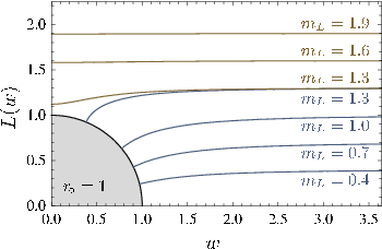
Note that the supergravity scalar is part of the radial coordinate of space. At asymptotically large values of the radial coordinate, where , the relation is . So at fixed near the boundary . In the inverse radial coordinate it scales like . According to the /CFT dictionary, the dual operator of the dimensional field theory therefore is of dimension . This operator is the bilinear . From holographic renormalization we learned that the mode of the solution scaling like is proportional to the source term of this operator. From the field theory Lagrangian we see that this source is the mass of the “quark field” . An exact calculation relates the parameter to the quark mass by11 1 Equation (2.76) does not look like the formula for given in the original paper, ref. [31], where the concept was introduced. The relative factor of arises from the different coordinate systems used here and in ref. [31]. The transformation between them introduces that factor in the embeddings and therefore also in the quark masses, cf. appendix A.
| (2.76) |
The embedding function in this way determines the mass of the quarks in the dual field theory [31].
Accordingly, the coefficient in (2.73) that scales like is proportional to the vacuum expectation value , known as the chiral condensate. We will not discuss this quantity in detail in this work.
2.3 Holographic quantum chromodynamics
In this section we want to point out some of the most important features of QCD and whether they can be described by gravity duals or not. We will see that the conditions at which the quark-gluon plasma exists, in particular finite temperature, allow for an at least qualitative description of many aspects via gravity duals.
The gauge/gravity correspondence is a remarkable tool for the investigation of the strongly coupled regime of gauge theories. Depending on the choice of parameters, the features of the gauge field theory will be more or less close to what we expect from quantum chromodynamics.
There is hope that the /CFT correspondence may provide some pre- and postdictions even though the exact gravity dual to QCD is not known. During the last years it turned out that there exist some quantities, like the celebrated ratio of shear viscosity to entropy density, that are universal in the sense that they do not depend on a particular supergravity background. Instead they are valid for all theories that have a gravity dual. If QCD is within this universality class, the results from other gauge theories than QCD may be applied to quantum chromodynamics as well.
Field content and supersymmetry
On the field theory side of the setup we stated that there is the gauge multiplet of super Yang-Mills theory supplemented by hypermultiplets. The gauge degrees of freedom show up in a multiplet together with scalar and fermionic superpartner particle fields. In the Maldacena limit these multiplet exists in infinitely many colors, i. e. the rank of the gauge group is infinite. The fundamental fermionic flavor degrees of freedom on the other hand exist only in a finite number of flavors, mostly we will restrict to . The models studied in the following do not explicitly break supersymmetry further, while other setups may allow to break supersymmetry completely [39].
Compared to QCD we deal with infinitely times more degrees of freedom. However, as we saw the large limit simplifies the theory drastically in the way that it allows us to neglect string loops. In fact corrections of results obtained from large expansions with expansion parameter tend to be small, as e. g. lattice calculations have shown.
Moreover, at all finite values of temperature supersymmetry is broken spontaneously. Unlike most other spontaneously broken symmetries it is not restored at high temperatures [40]. For a system at equilibrium this can be seen from the fact that the fermionic degrees of freedom contained in a supermultiplet obey antiperiodic boundary conditions along the imaginary axis in the complex time plane, while bosons are periodic. Therefore the Fourier decompositions and therewith the masses of these fields will differ. Fields with different masses however are not related to each other by supersymmetry transformations. This shows that supersymmetry is broken at finite temperature.
To great extent we will be interested in the behavior of fundamental matter and the bound states of the fundamental fields. As we have done above when we identified the mass of the quarks with the mass of the fundamental fermions in the hypermultiplet, we will think of these fields as the cousins of the quarks in QCD — keeping in mind that gauge invariant operators receive contributions from the scalar superpartners.
Conformal symmetry
By definition the /CFT correspondence relates gravity to a conformal, i. e. scale invariant, quantum theory. We introduced it as SYM theory. This is in vast contrast to QCD where we know several scales which break conformal symmetry.
The masses of the quarks which have to be regarded as fundamental parameters of QCD break scale invariance explicitly. The analogon to quark mass is realized geometrically in terms of the brane embedding profile.
The dynamically determined momentum scale at which the coupling constant diverges arises from quantization effects and therefore is a manifestation of scale anomalies. This scale has its dual in the background geometry of the supergravity theory. Temperature is geometrically realized by introducing a black hole into the spacetime of the gravity theory. The radius of the black hole introduces the scale dual to the finite temperature in field theory. In the way a finite temperature can be interpreted as a lower bound on the momentum of particles, the black hole horizon radius introduces a cutoff. We interpreted the radial coordinate in as the scale of a renormalization group flow. The horizon radius then works as a momentum cutoff. Geometrically, it introduces a scale and thereby explicitly breaks global conformal invariance.
Bound states of quarks
One of the great successes of the gauge/gravity duality is the possibility to derive spectra of bound states of fundamental matter from first principles. The string tension is a fundamental parameter of the theory and determines the quark mass, which naturally appears as a parameter in the spectra of bound states. Another parameter is the ’t Hooft coupling . Since we work in the low energy limit where we expect not to resolve the string scale we cannot explicitly assign any value to , and in the Maldacena limit we cannot assign a finite value to . We are thus unable to derive numerical values for meson masses. Nevertheless, the ratio of meson masses we obtain from holographic models can be compared to observations from experiment. Experimentally observed ratios of meson masses are reproduced with an accuracy of about 10% [41]. With respect to the various limits in which the according calculations are performed, this is an astonishing accuracy.
Baryons
The possibilities to model baryons is very limited to this day. This is partly due to the fact that we are restricted to the limit of infinitely many colors. Since baryons are colorless composite particles made out of quarks, we would have to describe an object made of an infinite number of particles.
Mesons
As mesons are composed operators containing one quark and one antiquark field, they transform in the adjoint representation of the flavor gauge group , which can also be expressed as a bifundamental representation with one index in the fundamental representation and the other in the antifundamenal , as we did in section 2.1 for the color gauge group. This transformation property on the string theory side is given by a string that has both ends on the probe D-brane. So the mesons of the field theory are dual to the excitations of D-D strings. The endpoints of these strings determine position of the probe D-brane. Consequently the excitations of the D-D strings describe fluctuations of the probe branes. The meson masses can then be obtained from the solutions to the linearized equations of motion of these fluctuations of the probe branes around the embedding.
As a very short sketch of the procedure and for later reference we outline the calculation of the spectrum of scalar mesons at zero temperature, first published in ref. [43]. Above, the embedding of the flavor D-branes at zero temperature was shown to be described by constant functions and constant . We now allow for small deviations from this embedding by adding small fluctuations to the embedding functions,
| (2.77) |
We want to consider small deviations from the brane profile and therefore may restrict our attention to the linearized equations of motion for the fluctuations . In the same way in which the embedding is determined by the equations of motion obtained from the DBI action, we can derive the linearized equations of motion for the fluctuations from the same action (2.65). Analogous to the derivation of the equation of motion (2.72) for the embedding functions the equations for the fluctuations around in the zero temperature case of are obtained by plugging in the ansatz (2.77) into the action. The resulting linearized equation of motion for the fluctuation was calculated in ref. [43] for zero temperature. To make the connection to the computation of the derivation of the embedding functions, we stick to the coordinates (2.68) with (2.69) in which the fluctuation equation for fluctuations are derived to be
| (2.78) |
Here is summed over the Minkowski directions, are the covariant derivatives along the directions of the spanned by the probe D-brane, and the radial coordinate of is given by . Use the ansatz
| (2.79) |
with as the spherical harmonics along the three sphere, such that . Here is the angular momentum number on the . However, in this work we only consider the solutions with . The plane wave factor is responsible for , with momentum vour vector which determines the meson mass by . Therefore the above ansatz transforms (2.78) into an ordinary differential equation for the radial part ,
| (2.80) |
It can be solved in terms of hypergeometric functions. However, normalizable solutions only exist for
| (2.81) |
where the quark mass enters through the embedding by (2.74) and (2.76), with constant . This is the mass spectrum of mesons at zero temperature and vanishing particle density. In fact this is the form of the spectrum for scalar, pseudo scalar and vector mesons [43]. We will compare later results at finite temperature and finite density to this formula.
Various aspects of meson spectroscopy have been under investigation, among these are the discrete meson spectra of stable quark-anti quark mesons at zero temperature [43], the decreasing stability and melting of these states at finite temperature and finite particle density [4, 3, 44], and the investigation of the spectra of heavy-light mesons [45, 46].
We will derive meson spectra for various purposes. On the one hand side we are interested in the dependence of the spectra under variation of temperature and particle density in order to understand the behavior of bound states of quarks. On the other hand we will observe the influence of external fields on the mass spectra to derive the polarizability of the mesons, which in turn influence their diffusion behavior inside the quark-gluon plasma.
Confinement/deconfinement
The probably most prominent feature of QCD is the running coupling constant, meaning the change in the value of the coupling constant of the strong interaction under variations of the energy scale of the interactions. Processes involving high momentum transfer are influenced less by the strong interactions that those which occur at low momentum. Mathematically, the value of the coupling constant even diverges at a momentum scale known as . Such a running of the coupling constant with respect to the energy scale is obviously only possible in the absence of conformal invariance, which would forbid the existence of a characteristic scale. As a result, quarks at low energies, e. g. low temperature, are confined to bound states which appear as colorless entities to a far away located observer. At high energies/high temperatures, the quarks may escape from these states and travel through spacetime independently.
Experiments show us that at energies above approximately 175 MeV quarks and gluons start to enter the deconfined regime. The exact value depends on various parameters. So far there is no analytic proof for these properties of quarks and gluons. To great extent this is due to the fact that the confinement/deconfinement transition occurs in the strongly coupled regime of the gauge theory. Traditional perturbative methods may not be applied here.
In the framework of the gauge/gravity duality, however, one can hope to see effects of the confinement/deconfinement transition, since we can work in the strongly coupled regime of the gauge theory. The original correspondence contained adjoint matter fields, given by the gauge multiplet of SYM theory. At finite temperature, the gauge fields undergo a first order phase transition at a temperature . It coincides with the Hawking-Page temperature and can be interpreted as the confinement/deconfinement transition [29, 47].
The fundamental matter existing in probe brane setups also exhibits a phase transition at finite temperature, which though occurs at a different temperature than the transition of the gauge fields. Various different models exist where the fundamental degrees of freedom indeed undergo a phase transition from stable bound states to dissociating ones [37, 38, 4, 44, 48]. We will come back to this transition when we discuss the QCD phase diagram in section 5.
It is interesting to note a difference between holographic and lattice models. The deconfinement temperature for fundamental matter associated with the destabilization of mesons derived from holographic models is proportional to the mass of the constituent quarks of the meson, . Lattice results in the quenched approximation, in contrast, suggest a scaling of the transition temperature of meson destabilization with the transition temperature for the gauge fields [49, 50]. This in principle allows for interesting comparison of lattice and holographic models with experimental data.
Chiral symmetry
Soon after the introduction of fundamental matter to the gauge/gravity duality it was shown that various probe brane setups are capable of realizing chiral symmetry breaking at finite temperature holographically [37, 38, 51, 52, 35]. The order parameter for the transition between the chiral symmetric phase and the phase of spontaneously broken chiral symmetry is given by the chiral condensate for massless quarks, i. e. the vacuum expectation value of the bifundamental . In some models this transition coincides with the confinement/deconfinement transition [53].
In the Sakai-Sugimoto model, chiral symmetry breaking is realized by the merging of the embeddings of the D and in the low temperature phase. In this way the flavor groups and originating from string excitations on the respective brane combine to a single vector subgroup .
3 Thermal vector meson spectra at finite particle density
In this section we address the first two questions raised in the introduction. We wondered whether bound states of quarks can be observed in holographic models of the thermal quark-gluon plasma, and how they are influenced by the medium. From experiment we know that temperature and particle density influence the interaction between particles, a prominent example is the transition of quarks and gluons from the confined to the deconfined phase at increasing interaction energy, or equivalently at high temperature.
Temperature and quark density are the most important parameters of the model we make use of in this work. Together with the mass of the fundamental fields they define the axes of the phase diagram of fundamental matter in the holographic QGP. In the context of gauge/gravity duality, there has been an intensive study of the phase diagram of supersymmetric Yang-Mills theory in the large limit, with fundamental degrees of freedom added by considering the -Schwarzschild black hole background with D-brane probes [54, 38, 37, 55, 56, 44]. Another approach was pursued by studying string worldsheet instantons [57]. Subsequently, particular interest has arisen in the more involved structure of the phase diagram when the baryon chemical potential is present, taking finite density effects into account [58]. We contemplate the phase diagram and its parameters more detailed in section 5. In this section we concentrate on the mesonic bound states of quarks and their dependence on temperature and density.
The aim of this section is the combination of both, finite temperature and finite density effects in the description of a thermal holographic plasma. In SYM theory with finite baryon density, we relate our work to the phase diagram shown in figure 2 of ref. [59], reproduced below in figure 3.1. We restrict to setups with non-vanishing particle density. Here, fundamental matter is described solely by probe branes with the geometry of black hole embeddings [58, 60]. The holographic realization of finite particle density is discussed below, where we introduce the setup.
The concept of mesonic bound states in SYM theory in the Maldacena limit at vanishing temperature and particle density, and an outline of how to obtain their spectra was sketched in section 2.3. Here, we extend these calculations to incorporate in-medium effects of finite temperature and particle density, giving rise to non-vanishing baryon or isospin chemical potential. The motivation to do so stems from the possibility to conduct experiments at non-vanishing isospin density [61], as well as the better accessibility by lattice methods of the finite isospin region in the phase diagram of QCD compared to finite baryon chemical potential. The work presented here restricts to the calculation of vector meson bound states with vanishing spatial momentum. At finite momentum the vector mesons couple to scalar mesons. Extensions of our work to finite momentum can be found in refs. [62, 63].
The meson spectra will be represented in terms of spectral functions. These functions of an energy variable will exhibit resonance peaks of finite width, corresponding to decay rates, at energies corresponding to the meson masses. The necessary extensions of the setup to finite particle density and the concept of spectral functions are introduced in the subsequent sections. In order to determine the spectral function at finite temperature and finite baryon density, we make use of the methods developed in the context of /CFT applied to hydrodynamics, c. f. for instance refs. [23, 64, 65]. For vanishing chemical potential, a similar analysis of mesons has been performed in ref. [48]. There it was found that the mass spectrum is discrete for quarks with masses significantly above the energy scale set by the temperature. At lower quark mass, a quasiparticle structure is seen which displays the broadening decay width of the mesons. As the mass decreases or temperature rises, the mesons are rendered unstable, reflected in broad resonance peaks. These excitations dissipate their binding energy into the plasma. Note that for this case, there are also lattice gauge theory results [66].
The achievements of the work presented in this section are the successful incorporation of either baryonic or isospin chemical potential at finite temperature. Before the results of this section where published as refs. [4, 3] these aspects where investigated separately in the literature. As we will see, the simultaneous incorporation of both temperature and particle density leads to spectra which can be compared to previous publications consistently in the appropriate limits. In particular, we find that at low temperature to quark mass ratio, i. e. close to the Minkowski phase, where the characteristic energy scale of the system is given by the quark mass, the spectrum is asymptotically discrete and coincides with the zero-temperature supersymmetric meson mass formula found in ref. [43] and rephrased in equation (2.81). However, away from this regime the dominant energy scale is either the finite temperature or the chemical potential. Here the observed spectra differ qualitatively from the above in some respects and resemble aspects of mesonic excitations in QCD. They also show interesting similarities to phenomenological models. We elaborate on the physical characteristics of our results in the summary of this section.
In the case of an isospin chemical potential, previous work in the holographic context has appeared in refs. [54, 67]. In this case, two coincident D-brane probes are considered, which account for fundamental matter of opposite isospin charge. We find that spectral functions quantitatively deviate from the baryonic background case. A triplet splitting of quasi-particle resonances in the spectral function is observed, which depends on the magnitude of the chemical potential.
3.1 Spectral functions
The spectral function of an operator describes the probability density in -space to detect the quantity encoded in the eigenvalues of the operator at given energy and spatial momentum . In our case, we want to describe quarkonium states and are interested in the mass/energy spectrum of the stable bound states and their lifetimes. In other words, we want to compute the spectral functions of a quark-antiquark operator corresponding to vector mesons. This operator appears in the field theory as the flavor current of fundamental fields (and their superpartners). For simplicity, let us restrict to the case of vanishing momentum, , where the remaining parameter is the energy alone. Peaks in the spectral function at an energy indicate that there is a large probability to find a quark-antiquark state, which is denoted as a quasiparticle if the width of the peak is small compared to the height. The position of the peak gives the energy or mass of the quasiparticle while the width of the peak translates into the lifetime of this particle in position space. According to Fourier transformation, a broad peak, which is a large object in momentum space, corresponds to an event of short lifetime in position space, and vice versa a narrow peak in the spectral function is a signal for a particle with a long lifetime.
We very briefly comment on how to derive the spectral function from two point functions, and how to extract the relevant information from them. See textbooks like ref. [68] for details. The formulation of spectral densities in terms of two point Green functions is convenient because we can compute the latter holographically.
We think of being the operator that describes the free mesonic quasiparticle as an excitation of one of the possible QGP many-particle states . There are infinitely many different of such states in the thermal ensemble that represents the QGP. The probability to occupy one of them is given by the density matrix , described in section 2.2.1. These states form a basis of the Hamiltonian of the ensemble, such that .
The probability of propagation from an initial spacetime point , which we define as , to some final point is given by the time ordered Green function
| (3.1) |
where the step function accounts for time ordering. The index shall remind us that this probability is not an ensemble average. It just gives the probability for the event if the QGP is in the state . By switching to the Schrödinger representation of the meson operators and denoting the momentum operator by ,
| (3.2) |
and insertion of a full set of eigenstates we arrive at
| (3.3) |
We denote the energy difference of the excited system to the QGP ground state as the energy of the mesonic excitation. This energy certainly depends on the state of the plasma with the excited mesonic state , and the state it was created from, . We write , and perform a Fourier transformation with respect to energy and momentum ,
| (3.4) |
where the small accounts for proper convergence. The delta function reflects that the momentum is conserved in the multiparticle system. To get the probability for the detection of a meson with energy and momentum in the QGP, we have to perform the ensemble average. This eventually leads to the relation
| (3.5) |
It is convenient to write this Green function as
| (3.6) |
Here, we defined a weight function for the propagation of the meson state, which assigns different probabilities to the propagation according to the Green function . The probability density is called the spectral density or spectral function. From (3.5) and (3.6) we see that the spectral function is given by
| (3.7) |
This notation reflects the physical interpretation we gave earlier. The probability to observe the multiparticle system in a state with a mesonic excitation, created by acting with on the initial QGP state , obeys energy and momentum conservation, and depends on the temperature, given by .
Most important for our purpose is the retarded Green function . We where not explicit about the retarded and advanced contributions to the Green function in the above discussion. Nevertheless, the Sokhatsky-Weierstrass theorem in complex analysis allows to derive the following relation between the spectral function and the retarded Green function that we will make use of,
| (3.8) |
The large probability density for the propagation of a quark-antiquark pair with the right energy content to form a bound state directly translates into an excess of the spectral function at that particular value of . In the rest frame of the particle, which we are restricting our attention to, the energy can directly be translated into the mass of the meson by . The calculation of the Green functions of flavor currents in this way yields information about the quasiparticle spectrum of a given theory — the meson spectrum.
From the relation (3.8), we see that a convenient way to obtain the spectral function is to compute the retarded Green function of the mesonic operator. A way to achieve this was sketched in section 3.1. We see that all information about the spectrum is contained in the correlation function . The correlation function in turn is determined by the residues of its poles in the complex plane. From field theory we know that the poles of the correlation function in the complex -plane can directly be translated to the energies of the states. We will consider spectral functions at vanishing spatial momentum , determined by the energy alone.
The standard example in field theory is Klein-Gordon theory which amounts to the equation of motion for a scalar field given by
| (3.9) |
In terms of the formalism of Green functions the evolution of a delta-shaped initial perturbation of is given by the inverse of the differential operator . The modes of this solutions are then obtained from the Fourier transform (with in our example of a particle at rest),
| (3.10) |
The Green function exhibits poles at , corresponding to modes with the energy of the stable particle at rest. These real valued poles are less frequently referred to as normal modes. The solution to more complicated systems than Klein-Gordon theory, where we have unstable excitations which dissipate energy, we encounter quasinormal modes which are complex valued. Quasinormal modes (QNM) where introduced in the context of metric fluctuations in black hole background. The black hole geometry accounts for the attenuation since any amount of energy that crosses the event horizon irreversibly disappears from the system outside. This mechanism also works in the case we will investigate. The difference to the simple example of Klein-Gordon theory is that we consider correlators of gauge field fluctuations in an black hole background rather than a scalar field in flat space. The fluctuations of the gauge field on the brane can transport energy into the black hole, but no energy can escape from the horizon. This introduces dissipation, which is then described by the imaginary part of the quasinormal modes.
For demonstration, presume the solution of the equation of motion for a mesonic excitation may be decomposed into quasinormal modes for complex frequencies . Suppose we only excite one mode for a single complex , such that . This mode describes an attenuated oscillation as long as the imaginary value of is negative,
| (3.11) |
For positive imaginary parts of the quasinormal modes, we encounter the unphysical case of infinite amplification of any fluctuation of the field. Therefore, in a physical setup one may find singularities of the retarded Green functions only in the lower half of the complex -plane. Those with the lowest absolute value of the imaginary part are referred to as the hydrodynamic poles of the retarded real-time Green function since they determine the long time behavior. Consider the made up example in which a Green function exhibits a pole at ,
| (3.12) |
The pole emerges as a peak in the spectral density of real valued energies ,
| (3.13) |
located at with a width given by . These peaks are interpreted as quasi-particles if their lifetime is considerably long, i. e. if and thus the peaks in the spectral function are narrow.
We compute the spectral function for real and complex values of the energy in this section. However, we focus on the meson spectra, i. e. the for , and postpone the discussion of the physical consequences and a detailed analysis of the behavior and location of the quasi normal modes to section 5. In-depth analytical and numerical investigations of the behavior of quasinormal modes in gauge/gravity duality can be found in refs. [69, 44].
3.2 Holographic setup
For an explicit calculation of the flavor current Green functions, we have to find the solutions to the equations of motion for the supergravity field, which is holographically dual to the flavor currents in the field theory. This field, which we called in the general example (2.58), is the gauge field on the probe brane [43]. This means that we have to include the contributions of the gauge field strength tensor in the DBI action.
Because of the non-linearity of the DBI action, the embedding functions and gauge fields couple. We no longer can expect to determine the embedding functions in terms of the quark mass alone. Instead, we first introduce a suitable coordinate system to describe the background geometry, then derive the equations of motion and solutions of the background fields, which are the embedding and the gauge field on the D-branes. In the subsequent section we investigate the fluctuations of the gauge fields on this background to eventually derive the meson spectra from them. To account for finite temperature, we consider finite values in the black hole metric.
We compute the functional dependence of the gauge field and the embedding functions numerically in the limit of vanishing spatial momentum for the fluctuations. In this limit the momentum four vector simplifies, and there are no couplings between the vector and scalar mesons.
3.2.1 Background geometry and supergravity action
We work in the D/D setup introduced above, i. e. we consider asymptotically space-time which arises as the near horizon limit of a stack of coincident D-branes. More precisely, our background is the black hole geometry discussed in section 2.2.1, which is the geometry dual to a field theory at finite temperature [22]. In this background, we encountered D-brane embeddings of Minkowski type as well as black hole embeddings. The phase transition between both classes of embeddings is of first order [37, 38]. The analysis of the meson spectrum shows that it corresponds to a transition between a phase of stable bound states of the fundamental degrees of freedom and a phase in which these mesons have finite lifetime. In physical parameters from the field theory point of view, we are in the deconfined phase at high temperatures at which mesons are unstable and said to be melting. For a well defined notion of high versus low temperatures, we need to compare the temperature to some energy scale. In our setup, the only available scale for comparison is the quark mass. Whether we are in the stable or in the melting phase, i. e. whether one or the other type of embedding is realized on the gravity side, depends on the ratio of quark mass to temperature , c. f. figure 2.4. This can be seen from the equation of motion for the embeddings (2.72). It is invariant under scale transformations by a factor of , resulting in , and . Scaling by amounts to scaling the quark mass by the same factor , while scaling of is equivalent to scaling the temperature by this factor. Because of the scale invariance of the equation of motion the functional behavior of the embedding, and therewith the physics of the D/D setup, is identical for all setups with the same ratio of quark mass and temperature. From (2.76) and (2.57) we infer
| (3.14) |
The free parameters of our setup appear on the right hand side as the asymptotic value of the D-brane embedding and the black hole horizon . The ratio of quark mass and temperature is defined by the ratio of these parameters, which we will henceforth denote by the dimensionless quantity
| (3.15) |
It was found that the transition to the melting meson phase occurs at a value of approximately [37]. At this value there is a change in the topology of the probe brane, which changes between the black hole type with a singularity and the regular Minkowski embedding. We demonstrated this in figure 2.4.
We use as the parameter which defines whether we are in the regime of high or low temperature. However, this will not affect the topology of the embedding in our setup. Below, we follow an argumentation which reveals that we may restrict to black hole embeddings, since this is the thermodynamically favored configuration in setups with finite particle density. Black hole embeddings are conveniently described in the coordinate system (A), derived in appendix A and also used in ref. [58],
| (3.16) |
with
| (3.17) |
In the following, some equations may be written more conveniently in terms of the dimensionless radial coordinate , which covers a range from at the event horizon to , representing the boundary of space.
As in section 2.2.2, we embed D-branes in this spacetime, such that they extend in all directions of space and along the directions of the three-sphere , which is part of the . Due to the symmetries of this background, the embeddings depend only on the radial coordinate and are parametrized by the functions . Due to our choice of the gauge field fluctuations in the next subsection, the remaining three-sphere in this metric will not play a prominent role. The induced metric on the D-brane is given by
| (3.18) |
Here and in what follows we use a prime to denote a derivative with respect to (resp. to in dimensionless equations). We write to denote the square root of the determinant of the induced metric on the D-brane, which is given by
| (3.19) |
Note that in general the branes are not necessarily coincident, and thus there will be one embedding function per brane, i. e. . We will make use of the DBI action to derive the embedding profiles . However, we postpone this task to the following subsection because the action also depends on the gauge field on the probe brane. We will see that the embedding function couples to this field on the brane.
Each of the branes features a “flavor gauge field” , with . This gauge field is arises from the fluctuation modes of an open string with both ends attached to the probe brane. For branes at arbitrary positions we therefore have an overall symmetry which is promoted to an in the case of coinciding branes. This symmetry enhancement comes from the fact that we then can no longer distinguish the branes and therefore cannot tell on which brane a string ends. Each of the two ends of a string can be assigned a label, also refered to as a Chan-Paton factor, which identifies the brane on which the string ends. There are possible configurations, matching the degrees of freedom of the non-Abelian symmetry group . The correct action for such a configuration of coinciding branes is given by the non-Abelian DBI action [70],
| (3.20) |
with as a placeholder for a spacetime index, and
| (3.21) | ||||
| (3.22) |
The Greek indices label the background spacetime coordinates, while Latin labels denote the directions perpendicular to the brane. Note that is a matrix with labels denoting solely these directions, and the determinant operator acts with respect to them. The determinant acts with respect to the labels of the directions along the brane. Additionally to this Lorentz structure, all the operators in the action above are elements of the algebra on which the symmetrized trace acts. The operators are operator valued analogon to the scalar embedding functions.
The non-Abelian nature of the embedding functions introduces non-commutativity of the spacetime coordinates. The physical consequences of the non-Abelian DBI action are not entirely understood by now. However, non-commutative spacetimes are candidates for the cure of UV divergences of quantum field theories and are applied in M-theory to describe spherical D-brane configurations [71]. The non-commutative contributions are manifest in (3.22), and hidden in the gauge covariant pullback of , which introduces gauge covariant derivatives of the embedding,
| (3.23) | ||||
with
| (3.24) |
where the indices are transverse and are along the worldvolume of the probe brane. The non-Abelian DBI action features commutator terms and of gauge fields and embedding functions. These commutator terms can be thought of as corrections to the Abelian DBI action, which is reproduced if the commutators in (3.22) and (3.24) are vanishing.
All setups we consider, feature a symmetry in the directions transverse to the D-branes which allows to set one of the two to zero, i. e. the embedding function in this direction is constantly zero. Thus, the commutators in (3.22) vanish. Moreover, we restrict to background configurations, arising from fields which are part of the Cartan subalgebra of . As a justification for this restriction, we claim our freedom to define a basis in the vector space of the algebra and choose the non trivial embedding to define the direction of the generator , which is the generator of . The embedding matrices thereby are diagonal. A usual interpretation of the Eigenvalues on the diagonal is that they give the embedding functions for each of the branes. The generators of the symmetry affect all flavor branes in an identical manner. The is therefore interpreted as the symmetry associated to baryon charge.
Recall that the embeddings determine the quark masses of the dual field theory. The construction of coinciding branes in our setup therefore implies that the flavor eigenstates coincide with the mass eigenstates of the particles in the dual field theory. Generalizations to distinct bases in the flavor and mass vector spaces should be possible.
In the following, we are especially interested in two different setups, both of which feature a vanishing Kalb-Ramond field but different . The case of allows investigation of the effects of baryon charge and the corresponding baryonic chemical potential. The symmetrized trace in the action is trivial in this case. The choice of features the diagonal generator proportional to which can be interpreted to charge the two flavors oppositely and therefore models isospin symmetry. The non-Abelian DBI action simplifies to
| (3.25) |
According to the arguments above, the matrix structure of and for is given by
| (3.26) | ||||
| (3.27) |
where we use the Cartan subalgebra of the , given by two Pauli matrices
| (3.28) |
All operators in the action therefore are diagonal. The two probe branes are coincident and the diagonal entries of the field strength tensor determine the net charges of the branes. We have
| (3.29) |
In any case, the restriction to the diagonal Cartan subalgebra of simplifies the non-Abelian DBI action, e. g. symmetrization of the trace is trivial in the sense that all commutators vanish and . Expansion of the square root and evaluation of the trace with subsequent restoration of the square root eventually leads to the following action for two D-branes in the black hole background with vanishing field,
| (3.30) |
We will concentrate on the cases of and , and separately switch on either the baryonic , parametrized by field strengths , or the isospin subgroup along the direction of , parametrized by the field strengths . Thus, the action for each brane is the same as long as we do not switch on both fields simultaneously.
To sum up, the background geometry described so far is dual to thermal supersymmetric Yang-Mills theory with additional hypermultiplets. These hypermultiplets arise from the lowest excitations of the strings stretching between the D-branes and the background-generating D-branes. The particles represented by the fundamental fields of the hypermultiplets model the quarks in our system. Their mass is given by the asymptotic value of the separation of the D- and D-branes. Since the physics of the thermal D/D setup is determined by the ratio of quark mass to temperature, we use the parameter , which is proportional to this ratio.
3.2.2 Background gauge fields — finite particle density
In addition to the parameter , we aim for a description of the system at finite baryon density , which in turn accounts for a finite chemical potential . In the thermal gauge theory, a baryon is composed of quarks, such that the baryon density can be directly translated into a quark density . The thermodynamic dual quantity of the quark density is the quark chemical potential , which is realized by a non-dynamical time component of the gauge field. The chemical potential is the source of the charge density operator , i. e. the time component of the current , of the particles charged with respect to the potential under consideration. The time component of the current of fundamental spin fields and the spin fields in the hypermultiplet is given by
| (3.31) |
In the dual holographic formulation the source of this charge density then corresponds to the non-renormalizable mode of the according holographically dual field in the supergravity theory. This field is the time component of the supergravity gauge field on the probe brane, which we denote by . The normalizable mode will yield the expectation value of particle density. We consider a constant chemical potential in space and time, i. e. there is no spacetime dependence. Instead we work with a gauge field background which only depends on the radial coordinate.
We do not rederive the dictionary entries here, but rather rephrase what is important for the following developments. The holographic interpretation of the embedding of the probe D-branes was discussed (in a different coordinate system) in section 2.2.2. The probe branes account for holographic duals of fundamental quarks with mass , determined by the non-renormalizable mode of the embedding function. The asymptotic form of the fields and can be found from the equations of motion in the boundary limit . The expansion coefficients in an expansion in powers of are given by
| (3.32) | ||||
| (3.33) |
Here is the quark chemical potential, is the quark density, is the dimensionless quark mass parameter given in (3.15) and is the quark condensate mentioned earlier (but irrelevant in this work). We made use of the dimensionless -coordinate that runs from the horizon value to the boundary at . The chemical potential and density of baryons are simply
| (3.34) |
Once we have found the solutions to the equations of motion for the gauge field, the value of the chemical potential in the dual field theory can be extracted as
| (3.35) |
where we introduced the dimensionless quantity for convenience. We apply the same normalization to the gauge field and distinguish the dimensionful quantity from the dimensionless
| (3.36) |
(we save the symbols without diacritics for later use). Analogously, the solutions of the embedding functions carry information about the quark mass parameter ,
| (3.37) |
We mentioned that for non-vanishing baryon density, there are no embeddings of Minkowski type, and all embeddings reach the black hole horizon. This is due to the fact that a finite baryon density in an infinite volume of Minkowski spacetime requires an infinite number of strings in the dual supergravity picture. These strings have one end on the stack of D-branes and the other on the stack of probe D-branes. These strings pull the brane towards the black hole [58]. Such spike configurations are common for configurations in which branes of different dimensionality connect [33].
Very recently, however, it was found that for a vanishing baryon number density, there may indeed be Minkowski embeddings if a constant vacuum expectation value of is present, which does not depend on the holographic coordinate [60, 59, 72, 73, 74]. The phase diagram found there is reproduced in figure 3.1.

In the shaded region, the baryon density vanishes () but temperature, quark mass and chemical potential can be nonzero. This low temperature region only supports Minkowski embeddings with the brane ending before reaching the horizon. In contrast, the unshaded region supports black hole embeddings with the branes ending on the black hole horizon. In this regime the baryon density does not vanish (). At the low- end of the line separating from in figure 3.1, there exists also a small region of multivalued embeddings, which are thermodynamically unstable [59]. In the black hole phase there is a phase transition between different black hole embeddings [58], resembling the meson melting phase transition for fundamental matter at vanishing density. This first order transition occurs in a region of the phase diagram close to the separation line between the two regions with vanishing (shaded) and non-vanishing (unshaded) baryon density. This transition disappears above a critical value for the baryon density given by
| (3.38) |
In this work we exclusively explore the region in which , i. e. we examine thermal systems in the canonical ensemble. For a detailed discussion of this aspect see refs. [60, 59].
To determine the solutions of the supergravity fields on the probe branes we have to extremize the DBI action (3.30), we write shortly as
| (3.39) |
The induced metric on the stack of coincident branes is given by (3.18), is the dimensionless field strength tensor of the gauge fields on the brane.
For now we consider the simpler case of a baryonic chemical potential modeled by the subgroup of . In this case, the sum amounts to an overall factor of . In ref. [58] the dynamics of such a system of branes and gauge fields was analyzed in view of describing phase transitions at finite baryon density. Here, we use these results as a starting point which gives the background configuration of the probe branes’ embedding function and the gauge field values at finite baryon density. To examine vector meson spectra, we will then investigate the dynamics of fluctuations in this gauge field background.
In the coordinates introduced above, the action for the embedding and the field strength is obtained by inserting the induced metric and the field strength tensor into (3.39). From now on we make use of the dimensionless coordinates and reproduce the action found in ref. [58]. To do so, we remember that the only non-vanishing component of the background field is the -dependent time component. Therefore, the only non-vanishing components of the field strength tensor are . We evaluate the determinant and arrive at
| (3.40) |
with components of the inverse metric . After inserting these components we get
| (3.41) |
where is the field strength on the brane. The background fields and depend solely on . This action only depends on derivatives of the gauge field. We therefore can identify the constant of motion satisfying ,
| (3.42) |
Evaluation of this formula and insertion of the asymptotic expansion of reveal that this dimensionless constant is related to the parameters of our setup by [58]
| (3.43) |
We can therefore think of the constant as parametrizing the baryon density .
The equations of motion for the background fields are conveniently obtained after Legendre transforming the action (3.41) to in order to eliminate dependence on the gauge field in favor of dependence on the constant of motion [58]. Varying this Legendre transformed action with respect to the field gives the equation of motion for the embeddings ,
| (3.44) | ||||
This equation for can be solved numerically for given and initial value . We impose boundary conditions such that the branes cross the horizon perpendicularly
| (3.45) |
Figure 3.2 shows some examples. The embeddings at finite density resemble the large asymptotics of the embeddings found at zero density. For small however, at finite particle density there always is the spike reaching down to the event horizon.

The initial value of determines the position on which the brane reaches the horizon and in this way determines the quark mass parameter , c. f. equation (3.37). It is zero for and tends to infinity for . Figure 3.3 shows this dependence of on for different values of the baryon density . In general, a small (large) is equivalent to a small (large) . For , we nearly observe proportionality. For vanishing , we only can model quarks with , heavier quarks at vanishing density are described by embeddings of Minkowski type, which we do not discuss here. (The trained eye can see that there is a maximum of in figure 3.3 before drops to smaller values towards . This is reflecting the existence of a phase transition to Minkowski embeddings at ).

The equation of motion for the background gauge field is given by
| (3.46) |
Integrating both sides of the equation of motion from to some , and respecting the boundary condition [58], we obtain the full background gauge field
| (3.47) |
Examples for the functional behavior of are shown in figure 3.4. While there is a significant slope of near the horizon at , the gauge field tends to a constant at large . From (3.35) we recall that this value is the chemical potential of the field theory. We will henceforth compute by evaluating the formula above for large . Note that at any finite baryon density there exists a minimal chemical potential which is reached in the limit of massless quarks.

3.3 Meson spectra at finite baryon density
3.3.1 Equations of motion
We now compute the spectral functions of flavor currents at finite baryon density , and temperature in the black hole phase. Compared to the limit of vanishing density treated in [48], we discover a qualitatively different behavior of the finite temperature excitations corresponding to vector meson resonances.
To obtain the mesonic spectral functions, we compute the correlations of flavor currents by means of the holographically dual gauge field fluctuations about the background given by (3.41). We denote the full gauge field by
| (3.48) |
According to section 3.2, the background field has a non-vanishing time component, which depends solely on . The fluctuations in turn are gauged to have non-vanishing components along the Minkowski coordinates only, and only depend on these coordinates and on . Additionally, the fluctuations are assumed to be small, such that it suffices to consider their linearized equations of motion. At this point we simply neglect the fluctuation of the scalar and pseudoscalar modes and their coupling to the vector fluctuations. This procedure is justified by the restriction to fluctuations with vanishing spatial momentum, which is imposed later. In this limit the vector mesons do not couple to the other mesonic excitations. A generalization of this work which includes these coupling and finite momentum spectra can be found in ref. [63].
The equations of motion are obtained from the action (3.39), where we introduce small fluctuations by setting
| (3.49) | ||||
| (3.50) |
The background gauge field is given by (3.46). The fluctuations now propagate on a background given by
| (3.51) |
and their dynamics is determined by the Lagrangian
| (3.52) |
with the fluctuation field strength . In contrast background field , the fluctuations do depend on the Minkowski directions as well as on the radial coordinate of . Since the fluctuations and their derivatives are chosen to be small, we consider their equations of motion only up to linear order, and derive these equations from the part of the Lagrangian which is quadratic in the fields and their derivatives. Denoting this part by , we get
| (3.53) |
Here and below we use upper indices on to denote elements of . The equations of motion for the components of are
| (3.54) |
The terms of the corresponding on-shell action at the -boundaries are (with as an index for the coordinate , not summed)
| (3.55) |
From this form of the action we can derive the correlation functions by means of the procedure outlined in section 2.2. First, we Fourier transform the fields as
| (3.56) |
As above, we are free to choose our coordinate system to give us a momentum vector of the fluctuation with non-vanishing spatial momentum only in -direction, .
To obtain the correlator with indices labeling Minkowski directions, we have to consider the second term in the parentheses of (3.55), including all its prefactors. Denote the resulting expression by . We decompose the gauge field fluctuations into a boundary and a bulk contribution, , where . The prescription from section 2.2 tells us to divide out the boundary terms from in order to get what was denoted by in (2.61). Once we found the solutions we can obtain this expression by evaluating
| (3.57) |
where the indices correspond to the Minkowski indices on .
To evaluate this expression, we have to insert the solutions to the equations of motion for into this expression. Note that on the boundary at , the background matrix reduces to the induced D-brane metric . Therefore, the analytic expression for boundary contributions to the on-shell action is identical to the one found in ref. [48]. In our case of finite baryon density, new features arise through the modified embedding and gauge field background, which enter the equations of motion (3.54) for the field fluctuations.
We adopt the procedure of ref. [48], where the coordinates in Minkowski directions where chosen such that the fluctuation four vector exhibits only one non vanishing spatial component, e. g. in -direction as . In addition, the action was expressed in terms of the gauge invariant field component combinations
| (3.58) |
In the case of vanishing spatial momentum , the Green functions for the different components coincide and were computed as [48]
| (3.59) |
where the in the denominator divides out the boundary value of the field in the limit of large . Again, the indices on the Green function denote the components of the operators in the correlation function, all off-diagonal correlations (as , for example) vanish.
In the limit of , the equations of motion for transverse fluctuations match those for longitudinal fluctuations . For a more detailed discussion see ref. [48]. As an example, consider the equation of motion obtained from (3.54) with , determining ,
| (3.60) |
Here we introduced the dimensionless frequency
| (3.61) |
In order to numerically integrate the equations of motion (3.60), we determine local solutions of that equation near the horizon at , which obey the infalling wave boundary condition. This condition ensures causality by demanding that the excitations can propagate in inward direction, but nothing can exit the horizon. The local solutions can be used to compute initial values in order to integrate (3.60) forward towards the boundary. The equation of motion (3.60) has coefficients which are singular at the horizon. According to mathematical standard methods, the local solution of this equation behaves as , where is a so-called ‘index’ of the differential equation [75]. We compute the possible indices to be
| (3.62) |
Only the negative sign will be retained in the following, since it casts the solutions into the physically relevant incoming waves at the horizon and therefore satisfies the incoming wave boundary condition. The solution can be split into two factors, which are and some function , which is regular at the horizon. The first coefficients of a series expansion of can be found recursively as described in [64, 65]. At the horizon the local solution then reads
| (3.63) | ||||
So, asymptotically assumes values
| (3.64) |
To calculate numeric values for , we have to specify the baryon density and the initial value , which determines the mass parameter . These parameters determine the embeddings appearing in (3.60). We can then obtain a solution for a given frequency by numerical integration of the equation of motion (3.60), using the initial values (3.63) and (3.64).
3.3.2 Spectra
We now discuss the resulting spectral functions at finite baryon density, and observe crucial qualitative differences compared to the case of vanishing baryon density.
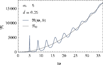
In figure 3.5 an example for the spectral function at fixed baryon density is shown. In the limit of large , corresponding to asymptotically small temperatures, the spectral function can be derived analytically. This zero temperature result is given by
| (3.66) |
Figure 3.5 shows this function as well.
All graphs shown here are obtained for a value of above , given by (3.38), such that we investigate the regime in which there is no fundamental phase transition of first order. Recall that the parameters of our theory are given by and . Therefore variations in the quark density at fixed temperature and quark mass are introduced by tuning only. The effects of different quark masses can be seen by tuning alone. The effect of changes in temperature involves changes in both and .
It is interesting to compare the spectra we obtain at finite temperature and density to the vector meson spectrum obtained at zero temperature and vanishing quark density. It is given by the same relation as the mass spectrum (2.81) which we encountered in the example of scalar mesons [43]. In our case, where the mesons do not carry spatial momentum, we can translate the mass of the excitation into an energy . At this energy we would see a resonance in a supersymmetric setup. In terms of the dimensionless quantities we use here, these resonance energies are given by
| (3.67) |
where labels the Kaluza-Klein modes arising from the D-brane wrapping the .
Finite temperature effects
We analyze finite temperature effects by choosing two values of and , which correspond to a given values of quark mass, quark density and a temperature . A change in temperature amounts to
| (3.68) |
and thereby leads to
| (3.69) |
An example is shown in figure 3.6.

| low T | , | blue line | |
| med. T | , | green line | |
| high T | , | red line |
There we plot spectra for three different temperatures, which we call low (, ), medium (, ) and high (,) temperature. We can see that at high temperature there is hardly any structure visible in the spectral function. However, we have chosen a temperature at which already a slight excitation is visible at low energies . Decreasing temperature leads to more and more pronounced peaks in the spectral function. Moreover, at decreasing temperature these peaks move closer to the resonance energies (3.67), corresponding to zero temperature and density (drawn as the corresponding dashed lines in the figure).
The formation of sharp resonances at low temperature indicates the intuitively expected behavior of long living mesons in a cold medium, which melt, i. e. decay faster, at high temperatures. However, we did not perform an analysis of the quality factor of the resonance peaks, i. e. we did not calculate the lifetimes of the vector mesons. From figure 3.6 we can see that the height-to-width ratio of the peaks seems not to improve to a great extent at low temperatures.
Finite density effects
To investigate the effects of finite baryon density , we tune while keeping constant. This amounts to varying the quark density at constant temperature and quark mass. The effect is shown in figure 3.7. We observe that the peak width is considerably influenced by baryon density. At low baryon density the resonances are close to line-like excitations, while they are broadened with increasing particle density. Additionally, increasing the particle density also causes a slight shift of the resonances to higher energies.
These observations are interesting from a phenomenologically inclined point of view. The in-medium effects on mesonic bound states are important to interpret the results of heavy ion collision experiments. Estimations from the early 1990s based on effective models predicted decreasing vector meson masses at increasing densities [76], known as Brown-Rho scaling. Experimental data from experiments at the SPS facility at CERN, however, is better described by models like the one found in refs. [77, 78]. There the in-medium effects also are reflected in peak broadening and shifts to higher energies.

For information on the spectral functions at vanishing particle density we refer the reader to ref. [48]. Where the low temperature regime for was investigated.
Dependence on quark mass
To observe the dependence on the mass of the quarks, we plotted spectra for different at constant values of in figure 3.8. We observe more and more pronounced resonances as we increase the meson mass. These mesons eventually nearly resemble the line spectrum (3.67) known from the supersymmetric case of zero temperature and vanishing quark density. This observation reflects the decreasing effect of finite temperature and chemical potential with increasing quark mass. In a regime where the scale of the quark mass outweighs both additional scales and their effects seem to be negligible. This is the case when we observe a configuration which is located close to the Minkowski phase in the phase diagram, cf. figure 3.1.
In ref. [4] we elaborate on the spectral functions behavior at low quark masses. There we observed that the position of the vector meson excitations in the regime of very low quark masses decreased with increasing quark mass. Further increasing the quark mass lead to increasing quark masses as described in this section. We omit this discussion here, but resume on the topic when we discuss the pole structure of the spectral functions. The reason is that the peaks referred to in ref. [4] are only visible after subtraction of the zero temperature part from the spectral function. To interpret the spectral function as a probability density for the detection of a quasiparticle, we cannot subtract , as we would otherwise produce negative probability densities, which are not well defined.
Our setup is a modification of the one used in ref. [48]. There, the authors considered vector meson spectra at vanishing baryon density. These spectra only show peaks moving to smaller frequency as the quark mass is increased. There is no contradiction to the results presented this work. Note that the authors of ref. [48] by construction are restricted to the regime of high temperature/small quark mass. Nevertheless, they continue to consider black hole embeddings below the temperature of the fundamental phase transition where these embeddings are only metastable, the Minkowski embeddings being thermodynamically favored. At small baryon density and small our spectra are virtually coincident with those of [48]. However, in our case, at finite baryon density, black hole embeddings are favored for all values of the mass over temperature ratio.

3.3.3 Pole structure
In this section we comment on the quasi normal modes (QNM) of the system under investigation. As discussed above, these are the poles in the complex frequency plane, i. e. the spectral function diverges at these locations. An impression of the continuation of the spectral function into the complex frequency plane is given in figure 3.10. The data to plot the graph was obtained in exactly the same way as for the spectral functions shown in the preceding sections, except the fact that we upgraded the numerics to process . Therefore the spectral functions shown so far are given by the values along the real axis.
Our numerics turn out to be reliable for and therefore cannot determine poles in the plane of which lie beyond this limit. We trust the values within the regions shown in the figures of this work, although there possibly is room for improvement in accuracy. We checked our code for stability against the initial conditions and parameters, and are mainly interested in the qualitative behavior of the results.
The spectra presented in preceding sections show that the first resonance peaks, i. e. those for small , are very narrow, while the following peaks show a broadening accompanied by decreasing amplitude. The physical consequence would be a longer lifetime of the lower excitations. This is reflected in a smaller imaginary part of the corresponding quasi normal mode in figure 3.10. It is a known fact that the quasinormal modes develop larger real and imaginary parts at higher . So the sharp resonances at low , which correspond to quasiparticles of long lifetime, originate from poles with small imaginary part. For higher excitations in at larger , the resonances broaden and get damped due to larger imaginary parts of the corresponding quasi normal modes.


Above we observed variations in the positions and widths of the peaks in the spectral function, depending on the changes in temperature, particle density and meson mass. This behavior can be translated into a movement of the quasinormal modes in the complex plane. Figure 3.10 shows the trajectory of the quasi normal mode corresponding to the first peak in the spectral function, parametrized by . At small densities, we can see the turning behavior of the mode which starts to move in the direction of decreasing real part at small , and then turns to asymptotically large real part while converging to the real axis for further increasing .
It would be interesting to compare our results to a direct calculation of the quasinormal modes of vector fluctuations in analogy to ref. [44]. There, the quasinormal modes are considered for scalar fluctuations exclusively, at vanishing baryon density. The authors observe that starting from the massless case, the real part of the quasinormal frequencies increases with the quark mass first, and then turns around to decrease. This behavior agrees with the peak movement for scalar spectral functions observed in ref. [48] (above the fundamental phase transition at ) where the scalar meson resonances move to higher frequency first, turn around and move to smaller frequency increasing the mass further. These results do not contradict the present work since we consider vector modes exclusively.
3.4 Meson spectra at finite isospin density
3.4.1 Equations of motion
In order to examine the case of two flavors, , with opposite isospin chemical potential in the strongly coupled plasma, we extend our previous analysis of vector meson spectral functions to a chemical potential with -flavor, i. e. isospin, structure. Starting from the general action (3.25) we now consider the non-Abelian field strength tensors
| (3.70) |
with the Pauli matrices and given by equation (3.48). The upper index on the gauge field labels the component in the vector space of the generators. The factor is due to the introduction of dimensionless fields as described below (3.35). The totally antisymmetric with arise from the structure constants of .
In the non-Abelian field strength tensor, the term quadratic in the gauge field describes a self interaction of the gauge field. The coupling constant for this interaction may be determined by a redefinition of the gauge field, such that the kinetic term of the effective four-dimensional theory has the canonical form. In appendix C (taken from ref. [3]) we show that the redefinition is given by
| (3.71) |
where the dimensionless constant depends on the geometry of the D worldvolume directions along and the , which are transverse to the directions of the D-brane. In particular, is independent of the ’t Hooft coupling . Determining the exact value of is left to further work in terms of the ideas presented in appendix C. In the following we chose a convenient . The field strength tensor in the redefined fields is given by
| (3.72) |
In order to obtain a finite isospin-charge density and its conjugate chemical potential , we introduce a -dependent time component of the valued background gauge field [5]. This background field is defining a direction in the vector space of the generators. We choose coordinates such that the direction of the background field aligns with the direction while the other components are vanishing,
| (3.73) |
This specific choice of the 3-direction in flavor space as well as spacetime dependence simplifies the isospin background field strength, such that we get two copies of the baryonic background on the diagonal of the flavor matrix,
| (3.74) |
The derivation of the background field configuration leads to the same explicit form of the action as (3.41). We can therefore make use of the background field solutions and found in the baryonic case. As before, we collect the induced metric and the background field strength in the background tensor .
For the fluctuations, however, we encounter an additional structure. The valued fluctuations in general have components along all the directions of this vector space. We make use of and apply the background field method in analogy to the baryonic case examined in section 3.3. As before, we obtain the quadratic action for the fluctuations by expanding the determinant and square root in powers of . The term linear in fluctuations again vanishes by the equation of motion for the background field. This leaves the quadratic action
| (3.75) |
The factor arises from the trace over the generators of . If we use the Pauli matrices as generators we get . Another common choice for the generators is , which amounts to . We leave the explicit choice open, since it merely introduces an unimportant finite proportionality constant to the action. Note that besides the familiar Maxwell term, two other terms appear due to the non-Abelian structure. One of the new terms depends linearly, the other quadratically on the background gauge field and both contribute non-trivially to the dynamics. The equation of motion for gauge field fluctuations on the D-brane is
| (3.76) |
with the modified field strength linear in fluctuations .
Integration by parts of (3.75) and application of (3.76) yields the on-shell action
| (3.77) |
The three field equations of motion (flavor index ) for fluctuations in transverse Lorentz-directions can again be written in terms of the combination . At vanishing spatial momentum we get
| (3.78) | ||||
| (3.79) | ||||
| (3.80) |
Note that we use the dimensionless background gauge field with . Despite the presence of the new non-Abelian terms, at vanishing spatial momentum the equations of motion for longitudinal fluctuations acquire the same form as the transverse equations (3.78), to (3.80).
Two of the above ordinary second order differential equations are coupled through their flavor structure. Decoupling can be achieved as22 2 At this point there is an essential difference which distinguishes this setup from the approach with a constant potential at vanishing mass followed e. g. in ref. [5]. While the metric coefficients for massless quarks are identical in both cases, there is a -dependence of the background gauge field in the present setup. in ref. [5] by transformation to the flavor combinations
| (3.81) |
The equations of motion for these fields are given by
| (3.82) | ||||||||
| (3.83) | ||||||||
| (3.84) |
with and dimensionless but -dependent . Proceeding as described in section 3.3, we determine the local solution of these equations at the horizon. The indices turn out to be
| (3.85) |
Since we are left with the same index as in (3.62) for the baryon case, i. e. the chemical potential does not influence the singular behavior of the fluctuations at the horizon. The local solution coincides to linear order with the baryonic solution given in (3.63).
For the special case of zero temperature the background geometry is . For finite chemical potential in the zero temperature case we can obtain the gauge field correlators in analogy to ref. [19]. The zero temperature result analog to (3.66) is given by
| (3.86) |
with the dimensionless chemical potential .
3.4.2 Spectra
Application of the recipe analog to the case of baryonic chemical potential yields the spectral functions of flavor current correlators in a medium with finite isospin density. Note that after transforming to flavor combinations and , given in (3.81), the diagonal elements of the propagation submatrix in flavor-transverse directions vanish, . Now the off-diagonal elements give non vanishing contributions. However, the component , longitudinal in flavor space, is not influenced by the isospin chemical potential, such that is nonzero, while other combinations with vanish [5].
In figure 3.11 we compare spectral functions for the isospin case, where we emphasize the first peak of each of the three components. Note that the spectrum coincides with the baryonic case, as the equation of motion (3.84) coincides with (3.60).

While the qualitative behavior of the isospin spectral functions agrees with the one of the baryonic spectral functions, there nevertheless is a quantitative difference for the flavor-transverse components . We find that the propagator for flavor combinations exhibits a spectral function for which the peaks are shifted to higher frequencies, compared to the Abelian case curve. For the spectral function computed from , the opposite is true, its peaks appear at lower frequencies. The quasiparticle resonance peak in the spectral function appears at higher frequencies than expected from the vector meson mass formula (3.67). The other flavor-transverse spectral function displays a resonance at lower frequency than observed in the baryonic case.
This may be interpreted as a splitting of the resonance peak into three distinct peaks. This is due to the fact that we explicitly break the symmetry in flavor space by our choice of the background field . Decreasing the chemical potential reduces the distance of the two outer resonance peaks from the one in the middle and therefore the splitting is reduced.
The described behavior resembles the mass splitting of mesons in presence of a isospin chemical potential expected to occur in QCD [79, 80]. A linear dependence of the separation of the peaks on the chemical potential is expected. Our observations confirm this behavior. Since the vector mesons are isospin triplets and we break isospin symmetry explicitly, we see that in this respect our model is in qualitative agreement with effective QCD models. Note also the complementary discussion of this point in ref. [81].
3.5 Summary
Two distinct setups were examined at non-zero charge density in the black hole phase. First, switching on a baryon chemical potential through non-zero baryon density, we find that nearly stable vector mesons exist close to the transition line to the Minkowski phase. Far from this regime, at small quark masses or high density, the spectral functions do not show distinct resonance peaks.
Moreover, at small quark masses and particle densities we observe that the quasi normal modes move to positions with smaller real part in the complex plane, in accordance with the observations in the case of vanishing chemical potential [48]. Increasing the quark mass over temperature ratio beyond a distinct value, the plasma adopts the behavior known from the case of zero temperature. In the spectral functions we computed, this zero-temperature-like behavior is found in form of line-like resonances, at low particle densities exactly reproducing the zero-temperature supersymmetric vector meson mass spectrum.
Besides finite temperature effects it is especially interesting to observe the in-medium effects caused by finite particle density. We observe a broadening width of the resonance peaks in the spectrum as a function of increasing particle density. At the same time, a slight shift of the resonance position to higher energies occurs. This result contradicts the expectations from the effective QCD models investigated by Brown and Rho [76]. However, experimental data from collision experiments at SPS do not support Brown-Rho scaling either. Instead more recent effective models, which are in good agreement with experimental data, also show a broadening of the -meson resonance peaks accompanied by a small positive mass shift [77, 78]. It would be interesting to investigate the mechanisms, that lead to the qualitative agreement of effective QCD models and the D/D setup that we observed here. Other in-medium effects will be studied in section 4.3. There we determine the mass shift of mesons due to polarization of mesons by the presence of the gluonic background field in the plasma.
Second, we switched on a nonzero isospin density, and equivalently an isospin chemical potential arises. The spectral functions in this case show a qualitatively similar behavior as those for baryonic potential. However, we additionally observe a splitting of the single resonance peak at vanishing isospin potential into three distinct resonances. This suggests that by explicitly breaking the flavor symmetry by a chemical potential, the isospin triplet states, vector mesons in our case, show a mass splitting similar to that observed for QCD [79]. It is an interesting task to explore the features of this isospin theory in greater detail in order to compare with available lattice data and effective QCD models [82, 83, 84, 85, 86, 87, 88, 89, 90]. In most of these approaches, baryon and isospin chemical potential are considered at the same time, which suggests another promising extension of this work. Moreover, in the context of gravity duals, it will be interesting to compare our results for the isospin chemical potential to the work presented in ref. [81].
Alternatively, instead of giving the gauge field time component a non-vanishing vacuum expectation value, one may also switch on -field components and combine the framework developed in [91, 92, 93] with the calculation of spectral functions for the dual gauge theory.
Our spectra also show that for given quark mass and temperature, lower meson excitations can be nearly stable in the plasma, while higher excitations remain unstable. At vanishing baryon density, the formation of resonance peaks for higher excitations has also been observed in [94].
4 Diffusion in the holographic plasma
Based on the observation that the many particle system observed at RHIC is well described by hydrodynamics with very low viscosity, the quark-gluon plasma is widely regarded as an almost perfect liquid [95, 96, 97]. In principle, the theory of hydrodynamics should be capable of modeling the collective dynamics of the plasma. This requires knowledge of initial conditions and the equations of state of the system. The hydrodynamic description then yields the dynamics of the system in terms of collective quantities such as currents, densities and entropy. For a comprehensive understanding of the quark-gluon plasma and related systems it would be pleasing to be able to derive the thermodynamic and kinetic properties of the system from first principles. In this section we present work which was conducted with the motivation to advance towards this goal. Adopting different points of view, we contemplate one particular attribute characteristic for fluids: diffusion.
The diffusion coefficient is a transport coefficient which parametrizes the ability of a fluid to reach an equilibrium state by transport of some initially unevenly distributed quantity through currents. In the quark-gluon plasma, these currents are the color and flavor currents, which account for the transport of quarks and gluons through the plasma. A particle of high diffusivity (high mobility) looses only a small part of its energy while traversing a given distance the medium and will transport its associated charge much faster than a particle which looses much momentum by interaction with the medium.
Close to thermodynamic equilibrium, transport coefficients such as that for diffusion can be derived from first principles by so called Kubo-formulae, which describe the coefficients in terms of correlation functions of the current which accounts for equilibration of the system. This approach has been used successfully in the past to derive transport coefficients and conductivities from holographic models [99, 100, 98, 101, 102, 103, 104, 105, 24, 106, 107, 108, 48].
In this section, once more the adjoint and fundamental matter described by the gauge multiplet of and the hypermultiplet of thermal SYM theory in the limit of a large number of gauge degrees of freedom serves as a model for the quark-gluon plasma.
The energy loss of heavy quarks and mesons in media has been a subject of intense experimental interest [109, 110, 111, 112, 113, 114, 115]. The suppression of charm and bottom quarks observed at RHIC motivated several groups to utilize the gauge-gravity duality [6, 13, 14, 8] to compute the drag of fundamental heavy quarks in super Yang-Mills theory at strong coupling [103, 100, 102]. In this approach, the heavy quark is given by a classical string attached to the D-brane probe. First studies of flavors in thermal /CFT beyond the quenched approximation, i. e. with non-zero , were performed in [116, 117].
We pick up the previous efforts and generalize them by including the effects of finite density, respectively chemical potential, on diffusion properties. The first part of this section very shortly addresses consequences of finite baryon density on a certain holographic method to derive the diffusion coefficient of baryons in a holographic plasma. Subsequently, in section 4.2, we study the gauge/gravity dual of a finite temperature field theory at finite isospin chemical potential. The isospin chemical potential is obtained by giving a finite vacuum expectation value to the time component of the non-Abelian gauge field on the brane, as in the previous sections. In order to obtain analytical results, we restrict our attention to the limit of massless quarks.
The consideration of an isospin chemical potential is an interesting field to study since it is still easier accessible by lattice calculations than setups at baryonic chemical potential. Hopefully holographic models one day allow for comparison to e. g. large lattice calculations. Moreover, isospin diffusion has been measured in heavy ion reactions [118, 61].
Eventually in section 4.3 we adopt a different point of view on diffusion in the holographic quark-gluon plasma. From the technical point of view, we do not pursue the approach of Kubo to obtain the diffusion coefficient directly from current correlation functions. Instead, we make use of a stochastic Langevin model, which determines the momentum broadening of particles due to random kicks from interactions with the medium.
Moreover, conceptually we extend the area of research on diffusion processes in the holographic QGP to mesons traversing the plasma. This effort bears two interesting aspects. One is the aim for a description of the kinetics of heavy mesons in the QGP, since observation show that heavy mesons like the survive the deconfinement transition. The other is the estimation of the effects of strong coupling on the plasma. The particular effective model we use does not rely on any weak or strong coupling limit for the interaction of the mesons with the medium. This allows for comparison of perturbative results for momentum broadening at weak coupling with holographic results for the strong coupling regime. In this way we present a method that may allow to estimate the effect of strong coupling on dynamic effects in the QGP.
4.1 Baryon diffusion
In this section, we calculate the baryon diffusion coefficient and its dependence on the baryon density in the thermal holographic plasma. The coordinates and parameters we use are the same as in section 3, they are discussed in detail in section 3.2.
In the context of holography, the idea is to describe the conserved current of the gauge field theory in terms of the dual gauge field in the supergravity theory, as we did in section 3. This current in our case is the current which transports baryon charge and therefore is non-zero when baryon diffusion occurs. The dual supergravity field was identified as the gauge field fluctuation on the probe brane. Any gauge field configuration of that satisfies the equations of motion also generates a conserved current in terms of the field strength , as . As in electrodynamics one can identify the columns of the field strength tensor with vector currents. Fick’s law of diffusion can be shown to be satisfied in the long distance limit for the on-shell field strength tensor of a supergravity gauge field. The constant is then identified with the diffusion constant [24]. This constant describes how strong the currents are which drive a hydrodynamic system into equilibrium, as a reaction on gradients in the charge distribution .
To solve for , one therefore has to find the solutions of the gauge field fluctuations which are holographically dual to the relevant current. As soon as a solution is found and gauge/gravity duality is invoked to compute the current , one may solve Fick’s law for . At vanishing particle density, the gauge field solution can determined from the DBI action in terms of metric coefficients alone [24]. Because we use the same coordinate system as the authors of ref. [48], we arrive at the same explicit form of the induced metric (3.18) on the probe D-brane in our setup. We therefore reuse the result for the diffusion coefficient derived there.
A very concise formula for the diffusion coefficient of R-charges was derived in reference to the membrane paradigm in ref. [24]. It was later directly translated to the diffusion of flavor currents in the D/D setup in ref. [48]. The name “membrane paradigm” does not refer to D-branes but instead alludes to the fact that the analogies between black hole physics and thermodynamics very often can be expressed in terms of events taking place at the event horizon (or slightly outside the horizon, then referred to as the “stretched horizon”), which has no materialistic manifestation but still appears as a significant surface, a membrane, to an observer or in the relevant formulae.
We extend previous efforts by introducing finite baryon density. This quantity explicitly enters the solution to the gauge field (3.47) which in turn explicitly enters the equation of motion (3.60) for the fluctuations. Therefore, one should expect a modified result for the diffusion coefficient including the explicit occurrence of the baryon density . We rely on the fact that these terms vanish for , restrict to the small density regime and stick to the expression found in ref. [48]. Nevertheless we still cover finite density effects in this way, since the probe brane embeddings are different for vanishing and finite density, as we see from their equation of motion (3.44). This difference should therefore translate into a dependence of the diffusion constant on the parameter , which is proportional to the baryon density by (3.43). We know that in the case of finite baryon density, black hole embeddings describe the entire parameter range of temperature and quark mass [60, 58].
Finally, the formula for the diffusion coefficient found in ref. [48] is given by
| (4.1) |
where the metric coefficients can be obtained from (3.18) with the square root of the absolute value of the metric determinant given by (3.19). Insertion of these coefficients and yields
| (4.2) |
The embeddings are determined as in section 3 by solving equation (3.44) in terms of the parameters for baryon density and initial value , which determines the quark mass normalized to temperature, c. f. figure 3.3.
The results for are shown in figure 4.1, where we compare to the result at vanishing baryon density found in in ref. [48]. There is a phase transition, at approximately which we briefly address in section 5.1.

The diffusion coefficient never vanishes in the medium with non-zero density. Both in the limit of and , converges to for all densities, i. e. to the same value as for vanishing baryon density, as given for instance in [24] for R-charge diffusion. In the regime of moderate to low temperatures the diffusion constant develops a nonzero minimum.
In order to give a physical explanation for this behavior, we focus on the case without baryons first. We see that the diffusion coefficient vanishes at the temperature of the fundamental deconfinement transition. This is simply due to the fact that at and below this temperature, all charge carriers are bound into mesons not carrying any baryon number.
For non-zero baryon density however, there is a fixed number of charge carriers (free quarks) present at any temperature. This implies that the diffusion coefficient never vanishes. Switching on a very small baryon density, even below the temperature of the phase transition, where most of the quarks are bound into mesons, by demanding there will still be a finite amount of free quarks. By increasing the baryon density, we increase the amount of free quarks, which at some point outnumber the quarks bound in mesons. In the large density limit the diffusion coefficient approaches for all values of , because only a negligible fraction of the quarks is still bound in this limit.
As a final comment, we point out that after the publication of these results in refs. [4, 3] a more careful analysis of the calculation of the diffusion coefficient was performed in ref. [119]. Here the diffusion coefficient was identified with the proportionality coefficient in the dispersion relation for the hydrodynamic quasi normal mode (the so called diffusion pole or hydrodynamic pole, cf. section 3.1) of the gauge field fluctuations at finite spatial momentum , given by
| (4.3) |
The inclusion of finite spatial momentum introduces several new aspects we circumvented in the limit of . In accordance with the results obtained from this analysis, the results for in the low quark mass/high temperature regime agree well with our naïve approach [119].
4.2 Isospin diffusion
We study the diffusion coefficient of particles charged under isospin chemical potential. The results where originally published as ref. [5]. Physically, the isospin chemical potential corresponds to the energy necessary to invert the isospin of a given particle. Within nuclear physics, such a chemical potential is of relevance e. g. for the description of neutron stars. In two-flavor QCD, effects of a finite isospin chemical potential have been discussed for instance in refs. [120, 85, 121].
In the following paragraphs we outline the procedure and comment on the restrictions we imposed. Recent work revealed that some of these can actually be considered as shortcomings. In particular the consideration of a constant background gauge field on the brane can be justified only for very small chemical potentials. Due to the assumed smallness of the chemical potential we neglected second order terms in the background gauge field on the brane. Both limitations however can be cured, based on the insights published in refs. [60, 58]. A reviewed version of our results can be found in ref. [122].
As in section 3, we introduce an isospin chemical potential by defining the vacuum expectation value of the gauge field on the coinciding probe D-branes to be
| (4.4) |
For simplicity, we work with a constant background field configuration. The above is a solution to the D-brane equations of motion and is present even for the D-brane embedding corresponding to massless quarks. However, We consider to be small, such that the Bose-Einstein instability observed in ref. [54], which is of order , does not affect our discussion here.
Even though, this constant gauge field given by (4.4) is a solution to the equation of motion, it does not represent the thermodynamically preferred configuration [60]. Instead we should rather make use of the solution presented in (3.47) with constant embedding function , for which the authors of ref. [60] present an analytical solution. Nevertheless, for simplicity we stick with (4.4) in this section, which may be justified in the case of very small densities, where the derivative of is very small, c. f. figure 3.4.
Again, we work in the D/D setup. For simplicity, we consider only the D probe embedding for vanishing mass . This embedding is constant and terminates at the horizon. This simplification allows us to derive our results purely analytically. We establish the non-Abelian action for a probe of two coincident D-branes and obtain the equations of motion for fluctuations about the background (4.4). These fluctuations are dual to the flavor current . We find an ansatz for decoupling the equations of motion for the different Lorentz and flavor components, and solve them by adapting the method developed in refs. [22, 23]. This involves Fourier transforming to momentum space, and using a power expansion ansatz for the equations of motion. We discuss the approximation necessary for an analytical solution, which amounts to considering frequencies with . With this approach we obtain the complete current-current correlator. The key point is that the constant chemical potential effectively replaces a time derivative in the action and in the equations of motion. In the Fourier transformed picture, this leads to a dependence of physical observables on the square root of the frequency. This non-linear behavior goes beyond linear response theory. We discuss the physical properties of the Green functions contributing to the current-current correlator. In particular, for small frequencies we find a frequency-dependent diffusion coefficient . Whereas frequency-dependent diffusion has — to our knowledge — not yet been discussed in the context of the quark-gluon plasma, it is well-known in the theory of quantum liquids and therefore may possibly also apply to the quark gluon plasma. For instance, for small frequencies the square-root behavior we find agrees qualitatively with the results of refs. [123, 124] for liquid para-hydrogen. Generally, frequency-dependent diffusion leads to a non-exponential decay of time-dependent fluctuations [125].
The approach used in this section is related but different from the procedure we implemented to obtain the spectral functions at finite isospin density in section 3. The non-analytical behavior we derive is due to the limits we consider. Coming from equation (3.85), the difference between a constant non-vanishing background gauge field and the varying one becomes clear. Here, the field is chosen to be small and constant in , such that terms quadratic in the background gauge field can be neglected. This implies that the square in (3.82) and (3.83) is replaced by , such that we obtain the indices instead of (3.85). If we additionally assume , then the under the square root can be neglected. In this case the spectral function develops a non-analytic structure coming from the factor in the index.
This section is organized as follows. We start with a comment on frequency-dependent diffusion within hydrodynamics and the method we use to compute the diffusion constant holographically. Thereafter, we establish the D probe action in presence of the isospin chemical potential, derive the corresponding equations of motion and solve them. Finally, we obtain the associated Green functions in the hydrodynamical approximation. From their pole structure we can read off the frequency-dependent diffusion coefficient. We comment on our results briefly where it is appropriate in this section and leave a summarizing discussion for section 4.4, including an interpretation of our results.
4.2.1 Diffusion coefficients from Green functions
Thermal Green functions have proven to be a useful tool not only to derive spectra, as above, but also for analyzing the structure of hydrodynamic theories and for calculating hydrodynamic quantities such as transport coefficients. In this section we once more use the gauge/gravity dual prescription of ref. [23] for calculating Green functions in Minkowski spacetime. These correlators can be thought of as being determined by their pole structure, in the way discussed in connection with the spectral functions, c. f. section 3.1. From these poles at complex frequencies we derive the diffusion coefficient of isospin charge with charge density and conserved current four vector .
Considering systems governed by hydrodynamics, such as the quark-gluon plasma, we are eager for solutions to the hydrodynamic equations of motion. Regarding diffusion, we pay special interest to the Green function for the diffusion equation
| (4.5) |
with the density, given by the time component of a diffusive current four vector , and is the diffusion constant we are interested in. In Fourier space this equation reads
| (4.6) |
This determines the dispersion relation of the mode with energy . In the language of Green functions we will observe solutions of the form
| (4.7) |
Here, the dispersion relation determines the poles of the Green function. Finding the correct dependence of the poles of the correlator on and therefore allows to determine the diffusion constant .
The diffusive quantity we are interested in the isospin charge with density as part of the four vector . These currents are holographically dual to the gauge field on the brane. We therefore have to solve the equations of motion for the gauge fields to obtain the relevant field theory Green function of isospin diffusion of by following the recipe for retarded correlation functions [23]. We are interested in the hydrodynamic properties and therefore restrict to the hydrodynamic long wavelength/low energy limit such that we restrict to the lowest order in .
For the non-Abelian case with an isospin chemical potential, in section 4.2 we will obtain retarded Green functions of the form
| (4.8) |
Retarded Green functions of this type have been discussed for instance in ref. [125]. Equation (4.8) describes frequency-dependent diffusion with coefficient , such that (4.6) becomes
| (4.9) |
In our case, is the isospin density at a given point in the liquid.
This is a non-linear behavior which goes beyond linear response theory. In particular, when Fourier-transforming back to position space, we have to use the convolution for the product and obtain
| (4.10) |
for the retarded Green function. This implies together with the continuity equation , with the three-vector current associated to , that
| (4.11) |
where denotes the convolution. This replaces the linear response theory constitutive equation . Note that for with constant, (4.10) reduces to (4.5).
4.2.2 Holographic setup
In this subsection we use the black hole coordinates given in appendix A, equation (A.4),
| (4.12) |
with the metric of the unit -sphere. This geometry is asymptotically with the boundary of the part at , the black hole horizon is located at .
Into this ten-dimensional spacetime we embed coinciding D-branes, hosting the flavor gauge fields . We choose the same embedding as in the previous calculations, which extends the D-branes in all directions of space and wraps an on the . Here, we restrict ourselves to the most straightforward case, that is the trivial constant embedding of the branes through the origin along the radial coordinate . This corresponds to massless quarks in the dual field theory. On the brane, the metric simply reduces to
| (4.13) |
Due to the choice of our gauge field in the next subsection, the remaining three-sphere in this metric will not play a prominent role. We use labels to denote any direction, to refer to Minkowski directions, is used as a label for the radial coordinate, and will be used to refer to the directions.
Introducing a non-Abelian chemical potential
A gravity dual description of a chemical potential amounts to a non-dynamical time component of the gauge field in the action for the D-brane probe embedded into the background given above. There are essentially two different ways to realize a non-vanishing contribution from a chemical potential to the field strength tensor . The first is to consider a -dependent baryon chemical potential, as we did in the preceding section. We work with a constant chemical potential of the form
| (4.14) |
where we sum over indices which occur twice in a term and denote the gauge group generators by . The brane configuration described above leads to an gauge group with on the brane, which corresponds to a global in the dual field theory. For , the generators of the gauge group on the brane are given by , with Pauli matrices . We will see that (4.14) indeed produces non-trivial new contributions to the action.
Using the standard background field method of quantum field theory, we consider the chemical potential as a fixed background and study gauge field fluctuations around it. We single out a particular direction in flavor space by taking as the only non-vanishing component of the background field. From now on we use the symbol to refer to gauge field fluctuations around the fixed background,
| (4.15) |
We gauge the component along the radial coordinate to and assume that for . Due to the symmetries of the background, we effectively examine gauge field fluctuations depending on the five-dimensional subspace on the brane spanned by the coordinates and by the radial coordinate . The magnitude of all components of and the background chemical potential are considered to be small. This allows us to simplify certain expressions by dropping terms of higher order in and in the chemical potential .
4.2.3 Equations of motion and their solutions
The action describing the dynamics of the flavor gauge fields in the D/D setup is the Dirac-Born-Infeld action. Since we work with vanishing gauge field components in all of the directions perpendicular to the D-branes, there are no contributions from the Chern-Simons action. As mentioned, we consider the constant D probe embedding corresponding to vanishing quark mass, . The metric on the brane is then given by (4.13). Since we are interested in two-point correlators only, it is sufficient to consider the DBI action to second order in ,
| (4.16) |
where we use the D-brane tension as in (2.14), performed the integration over the -directions, which are the directions along the , and the factor arising from the trace over the representation matrices ,
| (4.17) |
In our case we have .
Evaluating the DBI action given in (4.16) with the substitution rule (4.15), we arrive at
| (4.18) | ||||
where we use the short-hand notation and neglect terms of higher than linear order in , and higher than quadratic order in since both are small in our approach.
Up to the sum over flavor indices , the first term in the bracket in (4.18) is reminiscent of the Abelian super-Maxwell action in five dimensions, considered already for the R-charge current correlators in ref. [22]. The new second term in our action arises from the non-Abelian nature of the gauge group, giving terms proportional to the gauge group’s structure constants in the field strength tensor .
We proceed by calculating the retarded Green functions for the action (4.18), following the prescription of ref. [23] as outlined in section 2.2. According to this prescription, as a first step we consider the equations of motion obtained from the action (4.18), which are given by
| (4.19) | ||||
It is useful to work in momentum space from now on. We therefore expand the bulk gauge fields in Fourier modes in the directions,
| (4.20) |
As we work in the gauge where , we only have to take care of the components with .
For the sake of simplicity, we choose the momentum of the fluctuations to be along the direction, so their momentum four-vector is . With this choice we have specified to gauge fields which only depend on the radial coordinate , the time coordinate and the spatial direction.
Equations for - and -components
Choosing the free Lorentz index in the equations of motion (4.19) to be gives two identical differential equations for and ,
| (4.21) |
where we indicated the derivative with respect to with a prime and have introduced the dimensionless quantities
| (4.22) |
We now make use of the structure constants of , which are , where is the totally antisymmetric epsilon symbol with . Writing out (4.21) for the three different choices of results in
| (4.23) | ||||
| (4.24) | ||||
| (4.25) |
The first two of these equations for the gauge field directions transverse to the background field are coupled, the third longitudinal one is the same equation that was solved in the Abelian Super-Maxwell case [22]. Note that these equations are influenced by one of the addressed oversimplifications in a way that will turn out to be crucial at the end. We neglect terms quadratic in . If we would allow for these quadratic terms we could complete the square and avoid the non-analytical behavior we observe later [122].
Equations for - and -components
The remaining choices for the free Lorentz index in (4.19) result in three equations which are also not independent. The choices and give
| (4.26) | ||||
| (4.27) |
Solving (4.27) for , differentiating it once with respect to and using (4.26) results in equation (4.19) for ,
| (4.28) |
We will make use of the equations (4.26) and (4.27) which look more concise. These equations of motion for and are coupled in Lorentz and flavor indices. To decouple them with respect to the Lorentz structure, we solve (4.27) for and insert the result into the differentiated version of (4.26). This gives
| (4.29) |
The equations for are still coupled with respect to their gauge structure. The case was solved in ref. [22]. We will solve (4.29) for and can obtain from (4.27). Note that it is sufficient for our purpose to obtain solutions for the derivatives of the fields. These contribute to equations (2.58) to (2.61) that give the retarded thermal Green functions, while the functions themselves simply contribute a factor of which merely gives a factor of unity at the boundary.
Solutions
Generally, we follow the methods developed in ref. [22], and our differential equations are very similar to the ones considered there. Additionally, we need to respect the flavor structure of the gauge fields, only the equations for flavor index resemble those analyzed in ref. [22]. Those for involve extra terms, which couple the equations. Coupling occurs not only via their Lorentz indices, but also with respect to the flavor indices. We already decoupled the Lorentz structure in the previous section. As typical for an explicitly broken , the equations of motion which involve different gauge components will decouple if we transform to the variables
| (4.30) | ||||
Here, the , are the generally complex gauge field components in momentum space. Note that up to transformations, the combinations (3.81) are the only ones which decouple the equations of motion for . These combinations are reminiscent of the non-Abelian gauge field in position space,
| (4.31) |
The equations of motion for the flavor index were solved in ref. [22]. To solve the equations of motion for the fields with , we rewrite them in terms of and . Applying the transformation (3.81) to the equations of motion (4.23) and (4.24) and the versions of (4.29) and (4.27) leads to
| (4.32) | ||||
| (4.33) | ||||
| (4.34) |
where again and the upper signs correspond to and the lower ones to .
As in the section on spectral functions, we observe that some coefficients of these functions are divergent at the horizon . We hark back to the ansatz
| (4.35) |
with regular functions and . To cancel the singular behavior of the coefficients, we have to find the adequate and , the so-called indices, given by equations known as the indicial equations for and . We eventually get for all and
| (4.36) |
Note that these exponents differ from those of the Abelian Super-Maxwell theory [22] by a dependence on in the limit of small frequencies (). In the limit of vanishing chemical potential , the indices given in ref. [22] are reproduced from (3.62). Again, however, if we include the quadratic order in it is possible to complete the square to get [122].
In order to solve (4.32), (4.33) and (4.34) analytically, we introduce a series expansion ansatz for the function in the momentum variables and . In section 3.3.1 we solved the resulting equations up to first order in the radial coordinate in order to get initial conditions for the subsequent numerical integration. Here we are not interested in the dependence along , but in the dependence on the lowest order in and in order to extract the dispersion relation that determines the poles in the according correlators. In fact, the physical motivation behind this expansion is that we aim for thermodynamical quantities which are known from statistical mechanics in the hydrodynamic limit of small four-momentum . So the standard choice would be
| (4.37) |
On the other hand, we realize that our indices will appear linearly (and quadratically) in the differential equations’ coefficients after inserting (4.35) into (4.32), (4.33) and (4.34). The square root in and mixes different orders of . In order to sort coefficients in our series ansatz, we assume and keep only the leading contributions to and , such that
| (4.38) |
This introduces an additional order , which we include in our ansatz (4.37), giving
| (4.39) |
and analogously for the tilded quantities. If we had not included the resulting system would be overdetermined. On the other hand this procedure of including non-analytical square root terms would be superseded by including the second order terms in from the beginning. The results we obtain by using the approximations (4.38) and (4.39) have been checked against the numerical solution for exact with exact . These approximations are useful for fluctuations with .
Note that by dropping the in (3.62) we also drop the Abelian limit.
Consider the indices (4.36) for positive frequency first. In order to meet the incoming wave boundary condition, we restrict the solution to the negative sign only. For the approximate in (4.38) we therefore choose the lower (negative) sign. This exponent describes a mode that travels into the horizon of the black hole. In case of , we demand the mode to decay towards the horizon, choosing the lower (positive) sign in (4.38) consistently. Note that for negative frequencies the indices and exchange their roles.
Using (4.38) in (4.35) and inserting the ansatz into the equations of motion, we find equations for each order in and separately. After solving the equations of motion for the coefficient functions , , and , we eventually can assemble the solutions to the equations of motion for as defined in (4.30),
| (4.40) | ||||
and a corresponding formula for from the ansatz (4.35).
Illustrating the method, we now write down the equations of motion order by order for the function . To do so, we use (4.40) with (4.38) in (4.32) with the upper sign for . Then we examine the result order by order in and ,
| (4.41) | ||||
| (4.42) | ||||
| (4.43) | ||||
| (4.44) |
At this point we observe that the differential equations we have to solve for each order are shifted with respect to the solutions found in ref. [22]. The contributions of order in ref. [22] now show up in order . Their solutions will exhibit factors of order . Again, we emphasize that inclusion of terms would just result in a shift of .
Solving the system (4.41) to (4.44) of coupled differential equations is straightforward in the way that they can be reduced to several uncoupled first order ordinary differential equations in the following way. Note that there obviously is a constant solution for the first equation. Inserting it into (4.42) and (4.44) leaves us with ordinary differential equations for and respectively. Using the solutions of and in (4.43) gives one more such equation for .
To fix the boundary values of the solutions just mentioned, we demand the value of to be given by the constant and therefore choose the other component functions’ solutions such that , and the same for and . The remaining integration constant is determined by taking the boundary limit of the explicit solution (4.40), making use of the second boundary condition
| (4.45) |
see appendix B.1. Eventually, we end up with all the ingredients needed to construct the gauge field’s fluctuations as in (4.40).
We solve the equations (4.32) with lower sign for and (4.33) for and its tilded partner in exactly the same way as just outlined, only some coefficients of these differential equations differ. The solution for is then obtained from (4.34).
All solutions are given explicitly in Appendix B.1 together with all other information needed to construct the functions , , , , and .
4.2.4 Current correlators
In this section we obtain the momentum space correlation functions for the isospin currents by means of the holographically dual gauge field component combinations and defined in equation (4.30). Recall that the imaginary part of the retarded correlators essentially gives the thermal spectral functions (c. f. section 3). The following discussion of the correlators’ properties can therefore be related to the discussion of the corresponding spectral functions.
First note that the on-shell action gets contributions from the non-Abelian structure,
| (4.46) | ||||
where , and the index denotes the radial -direction. Up to the sum over flavor indices, the first term in the bracket is similar to the Abelian Super-Maxwell action of ref. [22]. The second term is a new contribution depending on the isospin chemical potential. It is a contact term which we will neglect. The correlation functions however get a structure that is different from the Abelian case. This is due to the appearance of the chemical potential in the equations of motion and their solutions. Writing (4.46) as a function of and results in
| (4.47) | ||||
In order to find the current correlators, we apply the method outlined in section 2.2 to (4.47), with the solutions for the fields given in appendix B.1. As an example, we derive the correlators and of the flavor current time components and , coupling to the bulk fields and , respectively. Correlation functions of all other components are derived analogously.
Green functions: Calculation
First, we extract the prefactor of from the action (4.16) and call it ,
| (4.48) |
We need this factor below to calculate the Green function,
| (4.49) |
The second step, finding the solutions to the mode equations of motion, has already been performed in section 4.2. In the example at hand we need the solutions and . From (4.40) and from appendix B we obtain
| (4.50) | ||||
| (4.51) | ||||
Note that we need the derivatives to apply (2.59) and (2.60).
Now we perform the third step and insert (4.48), (4.50) and (4.51) into (4.49). Our solutions and replace the solution and in (2.60). The resulting expression is evaluated at , which comes from the lower limit of the -integral in the on-shell action (4.47). At small , (4.50) and (4.51) give
| (4.52) | ||||
| (4.53) |
In the next to leading order of (4.52) and (4.53) there appear singularities, just like in the Abelian Super-Maxwell calculation [22, equation (5.15)]. However, in the hydrodynamic limit, we consider only the finite leading order.
Green functions: Results
Putting everything together, for the two Green functions for the field components , given in (4.30) by
we obtain
| (4.54) | ||||
| (4.55) |
These are the Green functions for the time components in Minkowski space, perpendicular to the chemical potential in flavor space. All Green functions are obtained considering hydrodynamic approximations in , neglecting mixed and higher orders .
The prefactor in (4.54), (4.55) is obtained using as in (2.14), from (4.17), and carefully inserting all metric factors, together with the standard /CFT relation . As in other settings with flavor [108], we concordantly get an overall factor of , and not , for all correlators. Contrary to those approaches, we do not get a factor of when summing over the different flavors. This is due to the fact that in our setup, the individual flavors yield distinct contributions. Most striking is the non-trivial dependence on the (dimensionless) chemical potential in both correlators. Note also the distinct structures in the denominators. The first one, (4.54), has an explicit relative factor of between the terms in the denominator. In the second correlator, (4.55), there is no explicit factor of . The correlator (4.54) has a complex pole structure for , but is entirely real for . On the other hand, (4.55) is real for but develops a diffusion structure for . So the correlators and essentially exchange their roles as changes sign. We find a similar behavior for all correlators and with . Once more, this behavior is a consequence of the insertion of and neglecting of terms of order in the hydrodynamic expansion (4.39).
We assume to be small enough in order to neglect the denominator term of order . Moreover, using the definitions of and from (4.22) we may write (4.54) and (4.55) as
| (4.56) | ||||
| (4.57) |
where the frequency-dependent diffusion coefficient is given by
| (4.58) |
We observe that this coefficient also depends on the inverse square root of the chemical potential . Its physical interpretation is discussed below in section 4.2.5.
In the same way we derive the other correlation functions
| (4.59) | ||||||
| (4.60) | ||||||
| (4.61) |
with the short-hand notation
| (4.62) |
Note that most of these functions are proportional to powers of and therefore vanish in the limit of vanishing spatial momentum . Only the -combinations from (4.59) survive this limit. In contrast to the Abelian Super-Maxwell correlators from ref. [22] given in appendix B.2, it stands out that our results (4.56), (4.57) and (4.59) and (4.61) have a new zero at . Nevertheless, bear in mind that we took the limit in order to obtain our solutions. Therefore the apparent zeros at lie outside of the range considered. Compared to the Abelian case there is an additional factor of . The dependence on temperature remains linear.
In the remaining -correlators we do not find any pole structure to order , subtracting an contribution as in ref. [22],
| (4.63) | ||||
| (4.64) |
We can see that the (with ) are purely imaginary for negative and real for positive . The opposite is true for , as is obvious from the relative factor of .
The correlators of components, pointing along the isospin potential in flavor space (), are found to be
| (4.65) | ||||
| (4.66) | ||||
with the diffusion constant . Note that these correlators have the same structure but differ by a factor from those found in the Abelian super-Maxwell case [22] (see also (B.36) and (B.38)). In particular the correlators in equation (4.65) do not depend on the chemical potential.
To analyze the novel structures appearing in the other correlators, we explore their real and imaginary parts as well as the interrelations among them,
| (4.67) | ||||||
| (4.68) | ||||||
| (4.69) | ||||||
| (4.70) |
Now we see why, as discussed below (4.57), and exchange their roles when crossing the origin at . This is due to the fact that the real parts of all and are mirror images of each other by reflection about the vertical axis at . In contrast, the imaginary parts are inverted into each other at the origin. The real part shows a deformed resonance behavior. The imaginary part has a deformed interference shape with vanishing value for negative frequencies. All curves are continuous and finite at . However, due to the square root dependence, they are not differentiable at the origin. Parts of the correlator which are real for positive are shifted into the imaginary part by the change of sign when crossing , and vice versa.
To obtain physically meaningful correlators, we follow a procedure which generalizes the Abelian approach of ref. [126]. In the Abelian case, gauge-invariant components of the field strength tensor, such as , are considered as physical variables. This procedure cannot be transferred directly to the non-Abelian case. Instead, we consider the non-local part of the gauge invariant which contributes to the on-shell action (4.46). In this action, the contribution involving the non-Abelian structure constant — as well as — is a local contact term. The non-local contribution however generates the Green function combination
| (4.71) |
We take this sum as our physical Green function. This choice is supported further by the fact that it may be written in terms of the linear combinations (3.81) which decouple the equations of motion. For example, for the time component, written in the variables given by (3.81), the combination (4.71) reads (compare to (4.47))
| (4.72) |
The contribution from is of order , while the combination for the first two flavor directions, , is of order .
We proceed by discussing the physical behavior of the Green function combinations introduced above. Their frequency dependence is of the same form as in the Abelian correlator obtained in ref. [22], as can be seen from (B.36). Since we are interested in effects of order , we drop the third flavor direction from the sum (4.72) in the following. It is reassuring to observe that the flavor directions , which are orthogonal to the chemical potential, combine to give a correlator spectrum qualitatively similar to the one found in ref. [22] for the Abelian Super-Maxwell action. However, we discover intriguing new effects such as the highly increased steepness of the curves near the origin due to the square root dependence and a kink at the origin — which have to be seen with skepticism because they vanish upon reinstating terms of order .
We observe a narrowing of the inverse resonance peak compared to the form found for the Abelian Super-Maxwell action (and also compared to the form of our . At the origin, the real and imaginary part are finite and continuous, but they are not continuously differentiable. However, the imaginary part of has finite slope at the origin. The real part though has vanishing derivative at .
The correlators , , and have the same interrelations between their respective real and imaginary parts as and . Nevertheless, their dependence on the frequency and momentum is different, as can be seen from (4.59) to (4.61). A list of the -direction Green functions split into real and imaginary parts can be found in appendix B.3.
4.2.5 Isospin diffusion coefficient
The attenuated poles in hydrodynamic correlation functions have specific meanings (for exemplary discussions of this in the context of /CFT see e. g. refs. [65, 127]). In our case we observe an attenuated pole in the sum at . The pole lies at . This structure appears in hydrodynamics as the signature of a diffusion pole located at purely imaginary . Its location on the imaginary -axis is given by the zeros of the denominators of our correlators as (neglecting )
| (4.73) |
Squaring both sides of (4.73) we see that this effect is of order . On the other hand, looking for poles in the correlator involving the third flavor direction , we obtain dominant contributions of order and (neglecting )
| (4.74) |
This diffusion pole is reminiscent of the result of the Abelian result of ref. [22] given in appendix B.2. As discussed in section 4.2.4, we consider gauge invariant combinations . In order to inspect the non-Abelian effects of order showing up in the first two correlators in this sum, we again drop the third flavor direction which is of order .
Motivated by the diffusion pole behavior of our correlators in flavor-directions corresponding to the combinations (see (4.73)), we wish to regain the structure of the diffusion equation given in (4.9), which in our coordinates () reads
| (4.75) |
Our goal is to rewrite (4.73) such that a term of and one term of order appears. Furthermore there should be a relative factor of between these two terms. The obvious manipulation to meet these requirements is to multiply (4.73) by in order to get
| (4.76) |
Comparing the gravity result (4.76) with the hydrodynamic equation (4.75), we obtain the frequency-dependent diffusion coefficient
| (4.77) |
Our argument is thus summarized as follows: Given the isospin chemical potential as in (4.4), (4.15), from (4.9) is the isospin charge density in (4.75). According to (4.75), the coefficient (4.77) describes the diffusive response of the quark-gluon plasma to a gradient in the isospin charge distribution. For this reason we interpret as the isospin diffusion coefficient.
Near the pole, the strongly coupled plasma behaves analogously to a diffractive medium with anomalous dispersion in optics. In the presence of the isospin chemical potential, the propagation of non-Abelian gauge fields in the black hole background depends on the square root of the frequency. In the dual gauge theory, this corresponds to a non-exponential decay of isospin fluctuations with time.
The square root dependence of our diffusion coefficient is valid for small frequencies. As long as , the square root is larger than its argument and at , the difference to a linear dependence on frequency is maximal. Therefore in the regime of small frequencies , which is accessible to our approximation, diffusion of modes close to is enhanced compared to modes with frequencies close to zero.
4.3 Meson diffusion at strong and weak coupling
In this section, we consider heavy mesons moving slowly through high temperature non-Abelian plasmas. In the context of transport properties of the holographic quark-gluon plasma we are mainly interested in the diffusion behavior of mesons. The central quantity we discuss here will however not be the diffusion coefficient, but its inverse, the momentum broadening coefficient , which determines the square of the momentum transfer per unit time, as we will see below.
The motivation for considering meson diffusion is twofold. First, future experiments at RHIC promise to measure the elliptic flow of mesons, and it is important to support this experimental program with theoretical work. To this end, various groups have studied the thermal properties of heavy mesons within the context of the /CFT correspondence [128, 129, 130, 101]. However, in spite of this progress, the transport properties of these mesonic excitations are not well understood. Although the kinetics derived in this work are not directly applicable to the heavy ion experiments, we believe that the results do hold some important information for phenomenology.
The second motivation for this work is theoretical. After the quark drag was computed using the correspondence, it was realized that the drag of quarkonium is zero in a large limit [128, 129, 130]. Since within a thermal environment the drag and diffusion of these mesonic states is certainly not zero, it remained as a theoretical challenge to compute the kinetics of these states using the /CFT setup.
As a central result, we compare the diffusion of mesons at weak and strong coupling. Using a simple dipole effective Lagrangian which does not rely on the value of the coupling, we calculate the in-medium mass shift and the drag coefficient of the meson in Super Yang Mills theory. At weak coupling we use perturbative methods, at strong coupling holographic models are employed. In the large limit the mass shift is finite while the drag is suppressed by . We reach the conclusion that relative to weak coupling expectations the effect of strong coupling is to reduce the momentum diffusion rate and thereby increase the relaxation time, which measures the time until the mesons in the plasma equilibrate their momentum spectrum to that of the thermal medium.
We also briefly pick up the discussion of in-medium effects on meson spectra, subject of section 3. There, the width of mesons in hot dense media was holographically determined by extending the analysis of meson melting to finite baryon density. In general the meson lifetime determined in this way is suppressed by the density of heavy quarks. However, we do not address the effects of finite density in this section. We are concerned with the thermal effects which capture the rescattering between the meson and the surrounding medium.
We focus on heavy mesons where the binding energy is much greater than the temperature. In this tight binding regime, mesons survive well above the critical temperature for deconfinement and the meson width is sufficiently narrow to speak sensibly about drag and momentum diffusion. This behavior was observed for holographic models in section 3.
For real charmonium, the binding energy can be estimated from the mass splitting between the and states, and for bottomonium from the and states with respectively [131]. Therefore it is not really clear that real quarkonia above – [132, 133] can be modeled as a simple dipole which lives long enough to be considered a quasi-particle. Indeed weak coupling hot QCD calculations of the spectral function show that over the temperature range –, the concept of a meson quasi-particle slowly transforms from being well defined to being increasingly vague [134, 135, 136, 137, 138]. There is lattice evidence based on the maximal entropy method (which is not without uncertainty) that and survive to and approximately respectively [139, 49, 50, 140, 141, 142]. However, model potential calculations which fit all the Euclidean lattice correlators indicate that the and survive only up to at most and respectively [143, 144]. Clearly, the word “survive” in this context is qualitative and means that there is a discernible peak in the spectral function. Given these facts, our assessment is that the dipole approximation might be reasonable for but poor for charmonium states and other bottomonium states.
An overview of this section is as follows. First, in section 4.3 we review the computation of drag and diffusion of heavy quark-antiquark bound states within the setup of perturbative QCD. This will outline a two step procedure to determine the drag coefficient at strong coupling.
The first step is to determine the in-medium mass shift (it is finite at large in the quantum field theory), which determines the polarizabilities of the meson. As expected from the dipole effective theory, the mass shift scales as , with the temperature and the inverse size of the meson. In the perturbative calculation, is the inverse Bohr radius, while in the /CFT computation the meson mass plays this role. In the field theory the dipole effective Lagrangian couples the heavy meson to the stress tensor and the square of the field strength, which we denote by the operator . In /CFT we obtain the mass shifts from the linear response of the meson mass by switching on the dual operators. This amounts to consider a black hole background or a non-trivial dilaton flow, respectively. For the dilaton flow we consider the D-D gravity background of Liu and Tseytlin [145]. This background and the -Schwarzschild background allow for an analytic calculation of the meson polarizabilities.
The second step is to compute the force-force correlator on the meson using the previously computed polarizabilities. This determines the drag coefficient and the momentum broadening as reviewed in section 4.3. This step requires the calculation of two-point functions involving gradients of the stress tensor and the field strength squared. Within gauge/gravity duality, these are obtained by considering graviton and dilaton propagation through the AdS-Schwarzschild black hole background.
Finally, we compare our results to perturbation theory and reach some conclusions for the heavy ion collision experiments in section 4.4.
A few passages of this section are adopted from ref. [2] as they stand. The phenomenological input and perturbative calculations as well as the numerical calculation of the Green functions by holographic methods where performed by D. Teaney, K. Dusling and C. Young during our collaboration on ref. [2]. The main contribution of the author of this work was the /CFT calculation in section 4.3.3, which is described in detail.
4.3.1 Effective model for heavy meson diffusion
We make use of a model for heavy mesons and their interaction with the quark-gluon plasma, which was introduced in ref. [146]. This effective model describes the interaction with the medium by a dipole approximation. It relies on the large mass of the meson relative to the external momenta of the gauge fields, i. e. the momentum scale given by the temperature of the medium, but does not rely on the smallness of the coupling constant. It was used previously to make a good estimate for the binding of to nuclei [146].
Because the model does not rely on the weakness of the coupling constant, we can make use of it in both the strong and weak coupling regime. At weak coupling we will refer to results from perturbation theory, while the results at strong coupling can be calculated from holographic duals. Since the exact dual to QCD is not known, we once more have to be satisfied with results for SYM theory. Therefore, we have to rephrase the model in terms of supersymmetric fields.
Diffusion in large QCD
The heavy meson field describes a scalar meson which has a fixed four-velocity . Then the effective Lagrangian for this meson field interacting with the gauge fields is [146]
| (4.78) |
where we refer to the last two terms as the interaction Lagrangian , and
| (4.79) | ||||
| (4.80) |
Here, is the non-Abelian field strength of QCD, with Greek letters as Lorentz indices and gauge index , The and are matching coefficients (polarizabilities) to be determined from the QCD dynamics of the heavy quark-antiquark pair. In inserting a factor of into the effective Lagrangian we have anticipated that the couplings of the heavy meson to the field strengths are suppressed by in the large limit.
In the rest frame of a heavy quark bound state with the operators and simplify to
| (4.81) | ||||
| (4.82) |
where and are the color electric and magnetic fields. If the constituents of the dipole are non-relativistic it is expected that the magnetic polarizability is of order relative to the electric polarizability. For heavy quarks, where is neglected, and large these matching coefficients were computed by Peskin [147, 148],
| (4.83) |
Here is the inverse Bohr radius of the mesonic bound state. It is finite at large since with and finite we have .
The effective Lagrangian can be used to calculate the in-medium mass shift. We will do so in the subsequent by simply consulting first order perturbation theory which says that
| (4.84) |
Translating the model to Super Yang-Mills theory
Our aim is to calculate the heavy meson diffusion coefficient from gauge/gravity duality. Subsequent to this subsection we explain the Langevin dynamics we use to describe this process, it requires the calculation of the two-point correlators as well as of the associated polarizabilities and . Because we do not now the gravity dual to QCD we translate the effective meson model to Super Yang-Mills theory, our standard toy model.
The formalism in Super Yang-Mills theory is not different from the one we introduced in the preceding section. In general all operators in SYM which are scalars under under Lorentz transformations and R-charge rotations will couple to the meson at some order. The contribution of higher dimensional operators is suppressed by powers of the temperature to the inverse size of the meson. The lowest dimension operator which could couple to the heavy meson field is , where denotes the scalar fields of the theory. However, the anomalous dimension of this operator is not protected, and the prediction of the supergravity description of SYM is that these operators decouple in a strong coupling limit [8]. The lowest dimension gauge invariant local operators which are singlets under and which have protected anomalous dimension are the stress tensor which couples to the graviton, and minus the Lagrangian , which couples to the dilaton. (Since we can add a total derivative to the Lagrangian, the operator is ambiguous. The precise form of the operator coupling to the dilaton is given in ref. [149]. We neglect this ambiguity here.) There also is the operator , which couples to the axion. An interaction involving breaks -symmetry, which is a symmetry of the Lagrangian of the hypermultiplet of the SYM gauge theory. Thus interactions involving can be neglected.
Summarizing the preceding discussion, we find that the effective Lagrangian describing the interactions of a heavy meson coupling to the operators in the field theory is
| (4.85) |
which is a linear perturbation of Super Yang-Mills theory. The two composite operators and in the interaction Lagrangian are
| (4.86) | ||||
| (4.87) |
They account for the interaction of the mesons with the background. In gauge/gravity duality the modification of the Lagrangian described by is achieved by considering the -Schwarzschild black hole background where . On the other hand, a finite is dual to a non-trivial dilaton flow described by Liu and Tseytlin in ref. [145]. Details follow below.
The polarization coefficients and will be determined below from meson mass shifts in gauge/gravity duality. This requires breaking some of the supersymmetry. We work in the linearized limit of small contributions from and . This allows to investigate the effects of finite temperature and background gauge fields separately. Additionally, this justifies the use of first order perturbation theory to compute the meson mass shifts in the medium as above by setting . For the contribution of the energy-momentum tensor, this is achieved by switching on the temperature. Then, the mass shift of the meson is given by expectation value of the stress tensor. Again we consider the rest frame of the mesons,
| (4.88) |
In contrast, for the meson response to the mass shift of a heavy meson is given by
| (4.89) |
Langevin dynamics
We now turn to the kinetics of the slow moving heavy meson with mass in the medium. The kinetic energy of the meson can be assumed to be of order of the temperature of the medium, such that . With we can estimate the velocity and momentum to be
| (4.90) |
For time scales which are long compared to medium correlations, we expect that the kinetics of the meson can be modeled as Brownian motion and can be described by Langevin equations. These are valid for times which are long compared to the inverse temperature but short compared to the lifetime of the quasi-particle state. We model viscous force and random kicks in spatial directions by
| (4.91) |
Here, is a component of the random force with second moment and is the drag coefficient. The solution for is given by
| (4.92) |
supposed that [150]. This allows to relate the drag and fluctuation by
| (4.93) |
This leads to the Einstein relation
| (4.94) |
One of the aims of this section is the calculation of the diffusion coefficients or , equivalently. From (4.91) we can obtain these coefficients once we know the microscopical phenomenological force
| (4.95) |
acting on the quasiparticle state. We can then compare the response of the Langevin process (4.91) to the microscopic theory (4.95). Over a time interval which is long compared to medium correlations but short compared to the time scale of equilibration we can neglect the drag, which is small for the heavy meson with . Since the considered time interval is long compared to medium correlations we can however equate the stochastic process, the random kicks , to the microscopic theory. We average (4.91)
| (4.96) |
In a rotationally invariant medium we have for
| (4.97) |
We now identify the force with the negative of the gradient of the potential that we read off from the Lagrangian or our theory, i. e. the interaction Lagrangian . For the case of QCD with only switched on we get
| (4.98) |
which is the usual form of a dipole force averaged over the wave function of the meson.
In our case is a constant in space and time, i. e. we consider situations with constant diffusion parameters in a homogeneous medium, for instance slight deviations from equilibrium. From the point of view of a more general description in Fourier space with we therefore are only interested in the hydrodynamic limit of . The fluctuation dissipation theorem relates the spectrum of (4.97) (with the specified time order of operators) to the imaginary part of the retarded force-force correlation function on the right hand side. In the hydrodynamic limit we get
| (4.99) |
where the full form of the retarded correlator is
| (4.100) |
Integrating out the heavy meson field as discussed in detail in ref. [100], which treated the heavy quark case, we obtain a formula for the momentum diffusion coefficient
| (4.101) |
with the retarded correlator given by
| (4.102) |
We can understand this result with simple kinetic theory. Examining the Langevin dynamics we see that is the mean squared momentum transfer to the meson per unit time. The factor of three arises from the number of spatial dimensions. In perturbation theory this momentum transfer is easily computed by weighting the square of the transferred momentum of each scattering with the transition rate for any gluon in the bath to scatter with the heavy quark,
| (4.103) |
Here, is the spatial momentum of the incoming gluon, is the momentum of the outgoing gluon and is the momentum transfer , and is the gluon meson scattering amplitude computed with the effective Lagrangian in (4.78) and weighted by the appropriate momentum distributions of the incoming and outgoing gluons,
| (4.104) |
Alternatively (as detailed in appendix A of ref. [2]), we can simply evaluate the imaginary part of the retarded amplitude written in (4.101) to obtain the same result.
In theory the generalized force is given by
| (4.105) |
which results in a momentum broadening
| (4.106) |
where the retarded correlators at vanishing velocity are
| (4.107) | ||||
| (4.108) |
In writing (4.106) we have implicitly assumed that there is no cross term between and . In the gauge/gravity duality this is reflected in the fact that at tree level in supergravity .
4.3.2 Weak coupling — perturbative results
We begin with the results for perturbative QCD (pQCD). The mass shift is obtained from first order perturbation theory as , yielding
| (4.109) | ||||
In the second line we have calculated the thermal expectation value in a free gluon gas and used (4.83).
The importance of this result is that it is finite at large and that it is in general suppressed by , i. e. by powers of the hadron scale to the temperature. If higher dimension operators were added to the effective Lagrangian their contributions would be suppressed by additional powers of .
For QCD the integrals written in (4.103) are straightforward and yield the following result for the rate of momentum broadening
| (4.110) | ||||
The high power of temperature arises since the dipole cross section rises as . The matching coefficient is directly related to the mass shift of the dipole and the inverse Bohr radius by (4.83) and (4.109). It encodes the coupling of the long distance gluon fields to the dipole. By taking the ratio between the momentum broadening and the mass shift squared, we find a physical quantity which is independent of this coupling
| (4.111) |
The large numerical factor originates from the cross section which grows as . A similarly large factor appears in SYM below.
For comparison with the /CFT result we list the results for super Yang-Mills theory in the limit of small ’t Hooft coupling , again computed in ref. [2],
| (4.112) | ||||
| (4.113) | ||||
| (4.114) |
4.3.3 Strong coupling — holographic calculation
We first determine the polarizabilities and from the mass shifts of the meson in two different backgrounds using (4.88) and (4.89). To accomplish this, we will switch on the perturbations of the Lagrangian which correspond to finite and finite . Again we consider the linear limit such that we can investigate the effects of finite temperature and finite background field strengths separately.
Subsequently we will compute the correlators in (4.107) and (4.108) for strongly coupled theory at finite temperature. The results we obtain in this section will be put together in the next subsection using (4.106) to deduce the rate of momentum broadening and compare it to the weak coupling result.
Backgrounds dual to finite temperature and field strength
The gravity background dual to SYM theory at finite temperature is given by the AdS-Schwarzschild black hole with Lorentzian signature. This background is needed below both for calculating the necessary two-point correlators and , as well as for obtaining the meson polarizability , which accounts for meson mass shifts due to finite temperature.
We make use of the coordinates derived in appendix A as (A.3) to write the -Schwarzschild background in Lorentzian signature as
| (4.115) |
In this way we can identify the transverse part to Minkowski space as nothing else than and we write it as
| (4.116) |
with the metric of the unit -sphere, and . The boundary is reached at asymptotically large while the horizon is located at . Notice that the black hole radius is related to the expectation value by [151]
| (4.117) |
The field configuration dual to and is a non-trivial dilaton background with has been given by Liu and Tseytlin and consists of a configuration of D-branes with homogeneously distributed D instantons [145]. The type IIB action in the Einstein frame for the dilaton , the axion , and the self-dual gauge field strength reads
| (4.118) |
The ten-dimensional Newton constant is given by
| (4.119) |
As can be seen from the supersymmetry transformations of the fermions, such a background breaks the supersymmetry to . Solving the equations of motion derived from (4.118), Liu and Tseytlin obtain the metric [145]
| (4.120) |
and axion-dilaton solution33 3 Regarding conventions, note that in our notation , where is used in the paper of Liu and Tseytlin [145].
| (4.121) |
The expectation value is given by
| (4.122) |
Computing the polarization coefficients from meson mass shifts
We again identify mesons with fluctuations of a D-brane embedded into the background dual to the field theory under consideration. Stable embeddings are obtained if the D-brane spans all Minkowski directions as well as the radial AdS coordinate and a -sphere in the remaining angular directions. Consider the metric (4.115) with (4.116) as an example. Here, the D-brane shall be embedded such that it spans all directions except and . The meson mass is then obtained by solving the equation of motion for the fluctuations [43], as outlined in section 2.3. Read as an eigenvalue equation, the equation of motion for the fluctuation gives the meson mass as the eigenvalues to the corresponding eigenfunctions . The discrete values of describe the Kaluza-Klein mass spectrum of mesons for any given quark mass.
To see this explicitly and generalize to the backgrounds of interest below, we rephrase this procedure for the vacuum case in a notation suitable for the subsequent generalization. Subsequently we will introduce a non-zero and , respectively.
In the case of a D-brane embedded in a ten-dimensional background, the brane embedding is described by the locations and in the two directions transverse to the brane. This setup was introduced in section 2.2. In general these locations depend on all eight coordinates of the eight-dimensional D-brane worldvolume and are determined by extremizing the DBI-action (2.65). We rephrase it here including the dilaton which we where free to set to unity in (2.65),
| (4.123) |
with the D-brane tension and is the string frame metric of the ten-dimensional background with coordinates . It is related to the Einstein metric as in (4.120). The distinction between the Einstein and string frame is ultimately important below to account for the effects of the non-trivial dilaton flow. The pullback contains the functions and , which are determined by solving their equations of motion, derived from .
The background dual to is obtained e. g. from (4.115) with . It is well known that for this background a probe brane embedding is given by the functions
| (4.124) | ||||
| (4.125) |
and the constant determines the quark mass . In terms of the example in section 2.2 this is instantly derived from the equation of motion (2.72) for the embedding in the zero temperature limit . Note however that there is a factor differing in the definition of the quark mass due to the choice of coordinates.
We are interested in the meson spectrum, which can be obtained from the brane fluctuations as in the previous sections, c. f. for instance page 2.3 in section 2.3. We thus allow for small fluctuations around this solution. Here we consider the fluctuation of the radial part , dual to the scalar meson excitations,
| (4.126) |
By the symmetries of the setup, the fluctuations only depend on the Minkowski directions and on the coordinate , denoting the radial coordinate on the part of the D-brane which is transverse to the Minkowski directions. The resulting equation of motion is analog to formula (2.78) (modulo the mentioned factors of ). The solutions were found by plugging in the ansatz
| (4.127) |
where are the scalar spherical harmonics on the wrapped by the probe D-brane and denotes a four vector. The resulting equation of motion for the function for reads
| (4.128) |
Here we introduced the following dimensionless quantities
| (4.129) |
where the dimensionless is not to be mistaken with the same symbol of different meaning defined in section 3. We moreover identified the meson mass squared with the square of the momentum four-vector of the fluctuations,
| (4.130) |
The eigenfunctions solving the Sturm-Liouville equation (4.128) are given in terms of the standard hypergeometric function ,
| (4.131) |
where and is a normalization constant such that
| (4.132) |
The lowest mode is given by
| (4.133) |
The corresponding eigenvalues to the functions are given by
| (4.134) |
We note that the mass of the lowest state with is
| (4.135) |
which will appear frequently below. For a more detailed derivation of these results the reader is referred to ref. [43].
Mass shift in the dilaton background
Let us now calculate the polarizability which determines the change of the meson mass at a given value of the gauge condensate with respect to the meson mass at ,
| (4.136) |
To find we will determine the mass shift and identify with the proportionality constant in front of .
We are interested in the eigenvalues of fluctuations in the case of . The ten-dimensional background geometry dual to this scenario is given in (4.120) and the equation of motion for D-brane fluctuations analog to (4.128) was derived in ref. [152] to be
| (4.137) |
with the dimensionless
| (4.138) |
To obtain analytical results, we consider the case of small and linearize in this parameter. Therefore the equation of motion to solve is
| (4.139) |
where the operator is given by
| (4.140) |
It is this term that describes the difference between the equation of motion at non vanishing background perturbation to (4.128), which is reproduced for .
To find the solution corresponding to the lightest meson with we set up a perturbative expansion. Any deviation from the solution of the case may be written as a linear combination of the functions , which are a basis of the function space of all solutions,
| (4.141) | ||||||
| (4.142) |
Plug this ansatz into the equation of motion (4.137), make use of (4.128) and keep terms up to linear order in the small parameters , and to get
| (4.143) |
We now multiply this equation by , integrate over and make use of (4.132) and (4.133) to see that
| (4.144) |
From we obtain
| (4.145) |
where in the last step we used (4.135) for the mass and (4.122) and (4.138) to relate and . By comparison with (4.136) we identify the polarizability
| (4.146) |
Mass shift in the finite temperature background
The calculation of the polarizability is completely analogous. We are now looking for the proportionality constant of meson mass shifts with respect to deviations from zero temperature, which we noticed to be given by
| (4.147) |
The background dual to the finite temperature field theory is the AdS black hole background given in (4.115) with (4.116).
Again we calculate the meson mass spectrum to identify the polarizability by comparison with (4.147). The embedding functions and in this background are given by
| (4.148) | ||||
| (4.149) |
where the quark mass is determined by . The function has to be computed numerically [37]. Some examples of such embeddings are shown in figure 2.4.
We introduce small fluctuations in the direction,
| (4.150) |
The linearized equation of motion for the fluctuations in the limit of vanishing spatial momentum and can be derived from the DBI action (4.123) to be
| (4.151) | ||||
where we abbreviated
| (4.152) |
In the regime of small temperatures, we may linearize in which is the leading order in . Furthermore, as may be seen from figure 2.4, in the regime of a small temperature compared to the quark mass , or respectively small ratios of , the embeddings become more and more constant. So for constant embeddings and up to order the equation of motion simplifies to
| (4.153) |
where we made use of the dimensionless quantities (4.138) and identify
| (4.154) |
For the lightest meson, the ansatz (4.141) this time leads to
| (4.155) | ||||
Reinstating units and solving for leads to
| (4.156) |
From this we can read off the polarizability as
| (4.157) |
Computing finite temperature correlators
According to (4.106) we need to compute the correlators (4.107) and (4.108) at finite temperature. We do so by once more performing the calculation along the lines of refs. [22, 23], sketched in section 2.2. The dual supergravity field to the energy momentum tensor is the graviton , and the corresponding field to the operator is the dilaton . Therefore, correlators of are associated with graviton propagation and obtained from the supergravity field solution to . Respectively, correlators of are associated with dilaton propagation and obtained from the supergravity solution to the dilaton . The calculational procedure for these two correlators is standard and has been discussed in refs. [23, 126], and first applied in ref. [22], in order to find two-point Minkowski correlators as discussed in section 2.2.
On the gravity side, both field correlators are computed in the black hole background to account for finite temperature correlation functions of the dual gauge theory operators. In this subsection it is convenient to work in the coordinates derived as (A.4), with radial coordinate . For an explicit calculation we are more specific here as in (2.61) by writing
| (4.158) | ||||
Here once more the function relates the boundary and bulk values of a gravity field to each other. For example the dilaton field is related to its value at the boundary by
| (4.159) |
and is normalized to one at the boundary, i. e. . For fluctuations of the metric component , is replaced by and the field theory operators in (4.158) are replaced by . The factor can be read off from the classical supergravity action
| (4.160) |
The classical five-dimensional gravity action for the graviton and dilaton is obtained from (4.118) as
| (4.161) |
where
| (4.162) |
So comparing to (4.160) we get
| (4.163) |
The equation of motion derived from (4.161) in momentum space reads
| (4.164) |
with dimensionless frequency and spatial momentum component . The prime denotes the derivative with respect to the radial coordinate . Note that in momentum space the function is akin to the radial part we denoted by above. The equation of motion (4.164) has to be solved numerically with incoming wave boundary condition at the black hole horizon. Computing the indices and expansion coefficients near the boundary , as done in refs. [64, 65], we obtain the asymptotic behavior as a linear combination of two solutions with asymptotic behavior for small as
| (4.165) | ||||
| (4.166) |
The general solution to the equation of motion therefore is given by the linear combination
| (4.167) |
where we normalized the functions such that the coefficient for is , which we are free to do since (4.164) is a homogeneous equation. In this way we achieve that the correct normalization for the radial part is implemented.
At the horizon the asymptotic solution satisfying the incoming wave boundary condition is
| (4.168) |
As discussed in refs. [64, 65] we find the coefficient by integrating the two boundary solutions from (4.167) forward towards the horizon and by matching the linear combination of the numerical solutions to the solution (4.168) at the horizon. We recognized that the solution of the radial part found in this way is equivalent to the radial part of the total solution and can therefore be plugged in for in (4.158).
The imaginary part of the retarded correlator then is given by
| (4.169) |
Solving (4.164) and matching the asymptotic solutions as described above, thus enables us to obtain
| (4.170) |
The corresponding result for the energy-momentum tensor correlator is obtained in an analogous way but the analysis is significantly more complicated. Fortunately it has been extensively and carefully analyzed in ref. [126]. The final result is
| (4.171) |
4.3.4 Comparing weak and strong coupling
We now have the results to compare momentum broadening of the heavy meson in a hot medium at weak and strong coupling. Over the duration of the lifetime of the heavy meson state it will loose momentum on average and simultaneously receive random kicks as codified by the Langevin equations of motion (4.91). The drag and momentum broadening rates are related by the Einstein relation
| (4.172) |
with the meson mass.
For strongly coupled SYM theory we obtain our principle result by collecting the results for polarizabilities (4.146), (4.157) and force correlators (4.170), (4.171), and use (4.106),
| (4.173) | ||||
The mass shift in strongly coupled SYM is given by the sum of the mass shift due to dilaton and graviton contributions, respectively. However, the exact value of the dilatonic mass shift (4.136) is determined by (4.122) in terms of , which we do not want to speculate about here. Nevertheless, from the definition of in ref. [145] we know that it is positive for positive instanton numbers. In this case the dilatonic mass shift contributes with the same sign as the graviton mass shift (4.147) and we write
| (4.174) | ||||
Here we made use of relations (4.157) and (4.117). Comparing these formulas with the analogous formulas in weak coupling large QCD given in equations (4.110) and (4.109),
| (4.175) |
and
| (4.176) |
we see that the meson mass plays the role of the inverse Bohr radius in the strong coupling dipole effective Lagrangian. This is as expected for relativistic bound states. Since these prefactors are different we do not compare the numerical values. Below we will compare the values of the ratio at strong and weak coupling. We moreover observe that the drag coefficient for heavy mesons is suppressed by in the large limit.
The phenomenological model we used modeled the interaction of the mesons with the medium as dipole interaction terms, which capture short distance phenomena. From the field theory side one may wonder if these dipole interactions indeed are the dominant interaction mechanism of the medium and the mesons. Considering /CFT, we admit that a dipole picture of a meson is a short distance description an we can not guarantee to describe such UV effects of the field theory well by holographic models. On the other hand, even if we cannot describe the interaction from first principle, the diffusion of the mesons and the scattering of gluons which then propagate with modified momentum into the medium is a long distance effect, which we can hope do describe by our approach. We therefore consider a quantity that is independent of short scale dipole interpretation of the medium, which is parametrized by the connection coefficients . To construct such a quantity, we remember from (4.106) that (for the simple case of )
| (4.177) |
Together with (4.88) we can then construct a quantity that does not depend on the connection coefficient ,
| (4.178) |
It is independent from the connection coefficient . All quantities in this expression have been calculated previously for weak coupling as well as for strong coupling. The strong coupling result is obtained from inserting the relations (4.117) and (4.171) and yields
| (4.179) |
To include the dilaton contribution, we make use of the above results (4.173) and (4.174) to get
| (4.180) |
It is then reasonable to use /CFT to estimate to what degree strong coupling physics modifies this ratio in QCD. In the free finite temperature theory, the result was computed in appendix A of ref. [2] and cited in (4.112) to be
| (4.181) |
Thus, comparing the strong coupling result (4.180) with the weak-coupling result (4.181), we conclude that strong coupling effects actually reduce the momentum transfer rate relative to the mass shift.
4.4 Summary
We studied transport properties of baryon charge, isospin charge and heavy mesons with three different methods. For the charge diffusion we derived the diffusion coefficient in dependence on temperature and particle density (or chemical potential, equivalently). In the case of meson diffusion in the quark-gluon plasma we observed how strong coupling effects the equilibration.
Baryon diffusion
We made use of the most naïve formulation of the membrane paradigm and derived a dependence of the diffusion coefficient for baryons that was qualitatively confirmed by recent and more comprehensive studies [119]. The results, shown in figure 4.1, indicate that for very large values of the baryon density, the diffusion constant asymptotes to its maximal value . This reflects the fact that in this case, the free quarks outnumber the quarks bound in mesons. For finite densities the diffusion coefficient is reduced and we observe a minimum at values of the quark mass to temperature ratio , which lie above the fundamental phase transition at zero density. We will draw a connection between the phase transition and the behavior of the diffusion in section 5.
Isospin diffusion
To obtain the isospin diffusion constant we analyzed the dispersion relation of the lowest lying quasi normal mode of the isospin current. We have considered a relatively simple gauge/gravity dual model for a finite temperature field theory, consisting of a constant isospin chemical potential obtained from a time component vacuum expectation value for the gauge field on two coincident brane probes. We have considered the constant D-brane embedding corresponding to vanishing quark mass.
Within the strong restrictions of our analytic derivation, the main result is that this model, despite its simplicity, leads to a hydrodynamical behavior of the dual field theory which goes beyond linear response theory. We find in particular a frequency-dependent diffusion coefficient with a non-analytical behavior. Frequency-dependent diffusion is a well-known phenomenon in condensed matter physics. Here it originates simply from the fact that due to the non-Abelian structure of the gauge field on the brane probe, the chemical potential replaces a time derivative in the action and in the equations of motion from which the Green functions are obtained. For a more comprehensive study one should include terms of quadratic order in the chemical potential , which then would cancel the non-analytic behavior.
Quarkonium diffusion
In the last part of this section we studied the diffusion of heavy mesons in the holographic plasma, by setting up a Langevin model. The forces on the meson where deduced from an effective dipole model for mesons that allowed to carry out our computations at strong and weak coupling. We therefore where able to estimate the effects of strong coupling on meson diffusion.
On the field theory side, we deduced the meson couplings to the stress tensor and the operator at strong coupling, which are the only relevant operators coupling to the heavy dipole. The couplings where deduced from mass shifts, which can be computed on the gravity side of the correspondence as a change in the normal vibrational modes of the D-brane in the presence of an external gravitational, or respectively dilatonic, field.
Because the gravitational and dilatonic fields shift the spectrum of the D-brane excitations, gradients such as those from fluctuations of these fields give rise to a net force on the mesonic modes. We used the fluctuation dissipation theorem to relate the spectrum of these fluctuations in the plasma to the momentum broadening of the meson.
The result for , the momentum broadening relative to the square of the in medium mass shift, for strongly coupled SYM theory is roughly four to five times smaller than the result in the weakly coupled limit. We therefore conclude that in this model the effect of strong coupling is to reduce the momentum broadening and increase diffusion of mesons relative to weak coupling.
From a phenomenological perspective the current calculation was limited to very heavy mesons, which survive above , where dipole interactions between the meson and the medium are dominant. It is certainly unclear if this is the relevant interaction mechanism above even for bottomonium. Furthermore, the dipole coupling between a heavy meson and the medium is dominated by short distance physics which is not well modeled by /CFT.
From the supergravity perspective, a better understanding of how gravitational and dilatonic fields fluctuate in bulk would give a straightforward procedure to calculate the drag of a finite mass meson. Specifically, fluctuations in the bulk would force motion of meson wave functions which extend into the holographic fifth dimension.
5 Exploring the phase diagram
While the theory of quantum chromodynamics is concise in its mathematical formulation, it exhibits a rich phenomenological structure, including several phase transitions. For instance, we frequently referred to the confinement/deconfinement transition quark matter is supposed to undergo when it is heated up and/or exposed to high chemical potential.
Since the development of QCD it was discovered that quark matter can exhibit numerous qualitatively different behaviors. The most prominent example in QCD is the change in the coupling constant of the strong interaction with respect to the momentum scale at which the theory is probed [153, 154]. It eventually accounts for the transition from the zero temperature regime (ground state with minimum momentum), where quarks are confined to the hadronic color singlets that make up the nuclei of atoms, to a deconfined state of matter at asymptotically high temperatures (and high thermal momenta) where quarks and gluons roam freely throughout spacetime. The value of the momentum interchange between quarks and gluons determines their interaction potential, which may change qualitatively, e. g. by increasing temperature, from a confining shape of infinite depth to a potential with finite binding energy.
Another example is the discovery of the so called color-flavor-locked phase of QCD with three color and three flavor degrees of freedom at high chemical potential, equivalent to high particle densities. It was observed that the thermodynamically favored ground state of QCD changes with the chemical potential. While we observe color and flavor symmetry separately for QCD at low chemical potential, there is some critical value of the chemical potential at which symmetry breaking occurs and a relation between color and flavor degrees of bound states of quarks is established [155, 156].
The motivations to explore the properties of QCD at high temperature and large chemical potentials include the struggle for a deeper understanding of the features of QCD itself, the formation of hadronic matter during the evolution of the universe and the description of matter inside dense astrophysical objects such as neutron stars.
We may wonder which parameters determine if we observe confinement and/or color flavor locking, which other symmetries and observables undergo qualitative changes and whether these changes occur abruptly or smoothly in the parameter space. This raises the question about the structure of the phase diagram of the theory. It describes the regions in the parameter space of the state variables in which the thermodynamic potentials and their derivatives behave analytically. The change from one phase to another is often accompanied by symmetry breaking and can be described by an order parameter which assumes finite values in one phase and vanishes in the other. For QCD, the quark condensate is frequently used as an order parameter. Non vanishing values break chiral symmetry. We can distinguish the hadronic phase, where , from the quark-gluon plasma with a higher amount of symmetry, here . However, strictly speaking the chiral condensate is non-zero in both phases for finite quark masses and should only be used as an order parameter in models with vanishing masses for the light quarks.
The exact overall structure of the phase diagram is not known yet. Especially at low temperature and chemical potential where the coupling is strong, theoretical treatments rely on lattice gauge theory, which on the other hand has its problems with modeling the QCD dynamics at finite temperature and finite baryon density. Figure 5.1 shows a sketch of the most basic features of the theoretically conjectured phase diagram of QCD based on combinations of analytical and numerical predictions [157, 158].

In huge volumes that exist for long periods of time, such as the cubic kilometer volumes of quark matter in neutron stars, one can expect the thermodynamic limit to be an appropriate approximation to describe matter, i. e. thermodynamics is applicable. As hydrodynamic models have successfully been applied to describe the collective motion of the fireball produced in heavy ion collisions, it is reasonable to assume that even the quark-gluon plasma observed in experiments reaches thermal equilibrium. The equilibration time is estimated to approximately , the plasma state then exists for about another [159]. Though in equilibrium, the multiparticle system in a collision experiment certainly does evolve along some trajectory in the phase diagram, which leads from some point in the QGP phase to a system of hadrons, which can eventually be detected.
For a thermodynamic description, the state variables can be chosen to be for instance the temperature , the pressure , and the chemical potentials for the different species of particles, labeled by the index . The chemical potential is the conjugate variable to the particle number . It is therefore only well defined if the number of particles of the species is well defined.
There are only a few charges that are conserved by all standard model processes. They allow for the definition of particle numbers and thereby determine the parameters of the phase diagram. These are quark number (which can be translated into baryon number), lepton number, electric charge, and color charge. Each of them has a chemical potential associated to it. In the processes we discuss in heavy ion collisions, there are no leptons (and in neutron stars they are radiated off by neutrino emission), i. e. the lepton chemical potential can be set to zero. The system furthermore is color-neutral, i. e. the chemical potentials associated to color charge can also be set to zero. The Gell-Mann-Nishijima-relation allows to rephrase the remaining parameters, quark number and electric charge, in terms of isospin and hypercharge. Hypercharge in turn is determined by the number of particles of the various quark species.
One may argue that in an equilibrium state weak interactions could account for flavor changing processes, and therefore there would be no well defined particle number associated to each quark flavor. As a result, the notion of a chemical potential would not be well defined. In heavy ion collisions however, the system in equilibrium state has not enough time to undergo weak interactions and therefore the flavor numbers are conserved, and the different quark flavors have to be assigned individual chemical potentials.
Thus, the remaining degrees of freedom in the phase diagram are temperature and the chemical potentials of the interacting quark species. In two-flavor setups, which we elaborate on in this work, we are free to express these potentials in terms of the baryon and isospin chemical potential. This is why we used and continue to use these charges as the parameters throughout this work. In principle we therefore consider a three-dimensional phase diagram in . For sake of simplicity, however, we restrict to cases of either non-vanishing baryonic or isospin chemical potential.
In the holographic context, several publications where dedicated to the investigation of the structure of the phase diagram of theories with gravity duals. For instance, the meson melting transition at finite temperature for the fundamental matter introduced by D-branes in a background generated by D-branes, was considered at zero as well at finite particle density. Studies of the behavior of D-brane probes in the Schwarzschild black hole background revealed a phase transition, which occurs when the D-brane reaches the black hole horizon. This transition was shown to be of first order in ref. [38], see ref. [52] for a similar transition in the D/D system, further details can be found in refs. [55, 56]. Related phase transitions appear in refs. [47, 160, 161]. Subsequently this phase transition was investigated at finite particle density [37, 58, 59]. The transition is characterized by a stable quasiparticle spectrum in one of the phases and melting mesons at finite density in the deconfined phase. Figure 3.1 illustrates the two phases. A way to derive the values of the transition line was mentioned in the same section, see the caption of figure 3.4 and ref. [59] for details. For the phase diagram in the model given by D- probes in a near horizon limit of D-branes with non vanishing chemical and isospin potential see ref. [67].
In this section we contribute to these studies by different means. In the subsequent section we observe a phase transition in the baryon diffusion coefficient and determine the critical baryon density at which this transition vanishes. The observations we make can be related to the results from refs. [48, 59] and confirm the observations described therein.
In section 5.2 we describe the occurrence of a new phase transition at finite isospin density, which we published in ref. [3].
5.1 Phase transition of the baryon diffusion coefficient
In this section we pick up the discussion from section 4.1, where we introduced a simple yet incomplete derivation of the baryon diffusion coefficient. As we mentioned there, the qualitative behavior of the result captures the physics correctly and the quantitative evaluation bears only little error in the regime of masses up to the temperature scale [119]. On the other hand, the evaluation of the simple formula (4.2) is a considerable simplification, compared to the exact treatment, described in ref. [119]. We will therefore stick with our approximation.
We focus on the temperature regime near the phase transition of fundamental matter. In the zero density limit, a phase transition of fundamental matter was observed to take place simultaneously to the geometric transition from Minkowski embeddings at small temperature to black hole embeddings at high temperatures. In the low temperature phase the mesonic spectral functions exhibit discrete delta peaks, and thereby describe stable mesons, while the spectrum becomes continuous with finite width peaks in the high temperature phase. The value of the quark mass to temperature ratio at which the phase transition can be observed was found to be near , c. f. figure 2.4. The transition can be seen as a first order phase transition in the quark condensate [37]. In the zero density limit the authors of ref. [48] observed another manifestation of the fundamental phase transition at as a phase transition in the baryon diffusion coefficient . We are interested in the finite density effect on this transition.
At finite density, we know that black hole embeddings capture the physics at all temperatures, i. e. the entire parameter regime of . The fundamental phase transition in this case is a transition between two different black hole embeddings [58]. As discussed in ref. [59], the baryon density affects the location and the presence of the fundamental phase transition. The transition is of first order only very close to the separation line between the regions of zero and non-zero baryon density shown in figure 3.1. Note that as discussed in refs. [60, 58, 59] there exists a region in the phase diagram at small and where the embeddings are unstable. This instability disappears for large .

We study the baryon diffusion coefficient at different baryon densities. Figure 5.2 shows the Diffusion coefficient as a function of the ratio of quark mass to temperature . By fixing the quark mass we may think of as the inverse of the temperature.
We find that the phase transition is slightly shifted towards smaller temperatures when we increase the density. At a critical density of the phase transition temperature is given by . Beyond the critical density the transition vanishes, in agreement with the critical density for the phase transition in the quark condensate, discussed in ref. [58].
5.2 A new phase transition at finite isospin potential
In this section we have a different look at the mesonic spectral functions, introduced in section 3. There we where interested in the behavior of the quasiparticle resonances and the modification of the particle spectrum when we leave the limit of zero temperature and vanishing particle density. Here, we focus on a new phenomenon occurring at high densities.
We recall that the three solutions , and to the fluctuation equations of motion (3.82) to (3.84) constitute the isospin triplet of mesons which may be constructed out of the isospin quarks of the field theory. This is analog to the -meson in QCD. We discovered that the mode coincides with the solution in case of a pure baryonic chemical potential, while the other two solutions have peaks in the spectral function at lower and higher values of , c. f. figure 3.11. The magnitude of this splitting of the spectral lines is determined by the chemical potential and the undetermined coupling .
In the limit of zero frequency , equations (3.82) and (3.83) coincide and will result in identical solutions and . In this limit the solution , though, differs from and , by means of the last term. So for small frequencies , we expect differences between the solutions and , . All three equations of motion depend on the particle density parametrically, since the density has influence on the background fields.
Spectral functions and quasi normal modes at high densities
We work in the canonical ensemble and will now investigate the effects of variations in . Spectral functions for various finite baryonic and isospin densities are shown in figure 5.3. As in section 3.3, the peaks in these spectral functions indicate that quarks form bound states. At low baryon densities we recognized the positions of the peaks to agree with the supersymmetric result (3.67). Increasing the quark density leads to a broadening of the peaks, which indicates decreasing stability of mesons at increasing baryon density [81, 162]. At the same time the positions of the peaks change, which indicates a dependence of the meson mass on the baryon density. Now, further increasing the quark density leads to the formation of a new structure at . We will discuss this structure below together with the results at finite isospin density.

We now turn to the effects of finite isospin density on the spectrum. The peaks in the spectral functions again correspond to mesons. An interesting feature at finite isospin chemical potential is the formation of a new peak in the spectral function in the regime of small at high density/high chemical potential, see figure 5.3. Notice that compared to the baryonic case, the density at which the new peak forms is about two orders of magnitude smaller. As in the baryonic case, the excitations related to the supersymmetric spectrum broaden, the corresponding mesons become unstable.
We pointed out that the structure of the spectral function is determined by the pole structure of the retarded correlator, see section 3.1. The poles of this function are located in the complex -plane at positions . The spectral functions show the imaginary part of the correlator at real valued . Any pole in the vicinity of the real axis will therefore introduce narrow peaks in the spectral function, while poles far from the real axis have less influence and merely introduce small and broad structures.
In section 3.1 we outlined how the imaginary part of the quasinormal modes describes damping, as long as . The short note on the pole structure demonstrated the dependence of the position of the quasinormal modes on the chemical potential/particle density. From figure 5.3 we deduce that at higher densities than studied so far, a quasinormal mode approaches the origin of the complex plane as the particle density is increased. We observe a pole at for a certain particle density , the value depends on . An impression of the variation in the spectral function is given in figure 5.5.
In figure 5.5 we qualitatively sketch the result from the investigation of the behavior of the quasinormal modes closest to the origin of the complex -plane. These modes do not produce the peaks corresponding to the spectrum (3.67).


At low densities all quasinormal modes are located in the lower half plane. When increasing the isospin density, the lowest frequency modes of the solutions and to (3.82) and (3.83) move towards the origin of the frequency plane. At the same time two quasinormal modes of move towards each other and merge on the negative imaginary axis, then travel along the axis towards the origin as one single pole. At the critical value of the modes from and meet at the origin, the quasinormal modes from still reside in the lower half plane. This observation matches the discussion at the beginning of this section, where we expected and to behave similarly at small , while should differ from this behavior. Upon further increasing the isospin density, the modes from and enter the upper half plane, maintaining their distinct directions. The sign change in from to indicates that a damped resonance changes into a self-enhancing one, and thus introduces an instability to the system. Figure 5.6 illustrates the transition of a quasinormal mode of from the lower half plane to the upper half plane. The -mode does not enter the upper half plane at any value of we considered. Compare this to the values of in figure 5.3 at which the pole induces visible structures at small . A comparable movement of poles in a different but related setup was found in ref. [163]. There the quasinormal modes of correlation functions of electromagnetic currents were investigated as a function of temperature.


In the following we interpret the observation of decaying mesons and the emergence of a new peak in the spectral function in terms of field theory quantities. In particular we speculate on a new phase in the phase diagram for fundamental matter in the D/D setup.
In the far UV, the field theory dual to our setup is supersymmetric, thus containing scalars as well as fermions, both of which contribute to the bound states we identified with mesons, even when supersymmetry is eventually broken. The meson decay at non-vanishing particle densities may be explained by the change of the shape of the potential for the scalars in the field theory upon the introduction of a non-vanishing density. As outlined in appendix D, a chemical potential may lead to an instability of the theory, since it induces a runaway potential for the scalar fields at small field values [164]. Nevertheless, interactions of -type lead to a Mexican hat style potential for larger field values. In this way the theory is stabilized at finite density while the scalar fields condensate. This squark condensate presumably contributes to the vev of the scalar flavor current,
| (5.1) |
In the /CFT context, the presence of an upside-down potential for the squark vev has been shown in ref. [54] using an instanton configuration in the dual supergravity background.
The occurrence of a pole in the upper half plane of complex frequencies at finite indicates an instability of the theory. A comparable observation was made in ref. [81], where in fact the vector meson becomes unstable by means of negative values for its mass beyond some critical chemical potential. The difference between this work and ref. [81] is that our model includes scalar modes in addition to the fundamental fermions. Nevertheless, in both models an instability occurs at a critical value of the chemical potential. The theory may still be stabilized dynamically by vector condensation [165]. In this case the system would enter a new phase of condensed vectors at densities larger than , in accordance with the expectation from QCD calculations [166, 88, 167].
We perform the analysis of the pole structure at for various , and interpret the phenomenon of the transition of poles into the upper half plane at finite critical particle density as a sign of the transition to an unstable phase. We relate the critical particle density to the according chemical potential by and use the pairs of and critical dimensionful to trace the line of the phase transition in the phase diagram of fundamental matter in the D/D setup. The result is drawn in figure 5.7. The picture shows the -plane of the phase diagram and contains three regions, drawn as blue shaded, white, and brown shaded, as well as solid lines, separating the different regions.

The blue shaded region marks the range of parameters, in which fundamental matter is described by D-branes with Minkowski embeddings. The line, delimiting the blue region, marks the line of phase transitions to the black hole phase, where fundamental matter is described by D-branes which have black hole embeddings. Using the symmetry of the DBI action, this phase transition line can be mapped to the line of phase transitions between Minkowski and black hole embeddings, present at finite baryon chemical potential [59, 60, 41].
The brown shaded region in the phase diagram in figure 5.7 marks the observation made in this section. The line delimiting the brown region marks the values of at which the pole in the spectral function appears at . Beyond this line we enter the brown shaded unstable region.
We observe that the separation line of the unstable phase asymptotes to a straight line at high temperatures. Within the values computed by us, this line agrees with the asymptotic behavior of the contour of particle density with , drawn as a thin gray line in the phase diagram. We thus speculate on a finite critical particle density beyond which the black hole phase is unstable. This interpretation is supported by analogous studies of the phase diagram of super-Yang-Mills theory with R-symmetry chemical potentials, where a similar line in the phase diagram was discovered [168, 169]. The remaining question is whether the brown shaded phase in figure 5.7 indeed is unstable in the sense that it inaccessible for any physical setup, or if there is a way to stabilize the system in the parameter range of question. Recent publications revealed that the introduction of a further vev for a different gauge field component on the stack of probe branes leads to a stabilization of the system [170, 171]. The resulting setup exhibits a second order phase transition to the new phase, which bears analogies to the theories of superfluidity and superconductivity [170, 172, 173, 171].
Note that the location of the transition line to the unstable phase in figure 5.7 as well as the results shown in figure 5.6 and figure 5.5 are obtained from the analysis of poles in the spectral functions. These functions in turn are obtained as solutions to equations (3.82) to (3.84), which do depend on the so far unknown factor in determining the self coupling of the gauge field on the brane. The computation of this factor is left to future work. It will determine the exact position of the boundary of the brown shaded region in figure 3.1. This will answer the question whether there is a triple point in the phase diagram and if the color shaded regions meet at a common border. Moreover, other poles than the ones investigated here may have influence on the stability of this system.
5.3 Summary
We made two observations concerning the thermodynamic behavior of fundamental matter in the D/D setup.
First, in our simple approximation of the baryon diffusion coefficient, we observe the fundamental phase transition and its dependence on the baryon density. We find that increasing the density from zero, where the transition temperature is given by , the transition temperature is lowered slightly until the transition vanishes at a critical value of , where the transition occurs at . This confirms the results of ref. [58], where the transition was observed in the quark condensate.
Second, we observe a new phase transition which renders the D/D setup unstable at values above a critical isospin density. This becomes manifest by quasinormal modes of the fluctuations which develop positive imaginary parts in this region of the phase diagram. The exact position of the phase transition line cannot be determined yet. However, we speculate that the instability is due to a modification of the potential for the scalar fields in the field theory. This instability can be cured by vector meson condensation.
It is tempting to compare figures 5.7 and 5.1. However, we point out that we cannot interpret the brown shaded region in fig. 5.7 as a direct analogon of the color-flavor-locked phase (CFL) in fig. 5.1, since the parameter range scanned by us only allows to observe the phase transition to the new phase only at finite isospin chemical potential and not at finite baryon potential. Also the critical point at finite is not reproduced so far from the thermodynamics of the D/D model. Nevertheless, the sheer appearance of the phase diagram in figure 5.7 may serve as a motivation for further efforts in exploring the phase diagrams of holographic models.
6 Conclusion
We considered different generalizations of the /CFT correspondence in order to shed light on in-medium effects on the fundamental matter in holographic models for the quark-gluon plasma. The influence of the medium was parametrized by the values of the temperature and particle density.
The first aspect we considered in 3 was the influence of the medium on bound states of quarks, in particular vector mesons. The description of mesons from first principles is interesting in its own right, because the strong coupling parameter forbids to apply well established perturbative methods in QCD. In the holographic setups, mesonic excitations arise more or less naturally as vibrational modes of open strings on D-branes. In the low energy limit, they account for fluctuations of supergravity fields. We presented the capabilities of a certain realization of a D/D brane configuration by deriving the spectral functions for vector mesons from it. In the limit of vanishing temperature and density the derived spectra agree with the previously known results. The main achievement of our efforts, however, was the extension of the spectral description of vector mesons into the finite density and temperature regime for all values of quark masses and temperature. We observe the melting of mesons at high temperature and at the same time studied the effects of finite particle density. Technically, we related the characteristics of the spectra to the behavior of the quasi normal modes of the excitations that holographically account for mesonic bound states of quarks.
The main contribution to a better understanding of in-medium effects from this project is the derivation of in-medium effects on the spectra. We observe a destabilization of mesonic bound states with increasing particle density in the quark-gluon plasma, which is simultaneously accompanied by a slight shift of the meson masses to higher energies. Due to the fact that the holographic models are too complex to be solved by analytical methods alone, the precise mechanisms that account for this behavior are difficult to reveal. A probable physical explanation for the destabilization certainly can be seen in the fact that in the strongly coupled medium the surrounding free quarks alter the binding interquark potential of the mesonic bound state. The closer a quark of the medium comes to a constituent quark of the meson under consideration, and the higher the amount of such perturbing spectator quarks is, the more influence can be expected from the medium on the mesons. Therefore increasing the baryon density (which can be seen as a measure for the amount of free quarks in the medium which are not bound into mesons) accounts for accumulating perturbation of the binding quark-antiquark potential, eventually leading to a dissociation of the meson. The shift in the meson mass may also be a consequence of the modification of the interquark potential, which in turn shifts the binding energies and therewith the energy content of a meson.
Without speculating further on the mechanisms that lead to the observation we made, we note that our results are in qualitative agreement with phenomenological models and observation from experiment. The fact that our result is a non-trivial consequence derived from the D/D setup can be seen as an affirmative answer to the question whether string theory motivated models can capture phenomenologically relevant physics.
Another such example was also derived in the context of meson spectra. Namely, we have shown that the introduction of finite isospin chemical potential indeed leads to a mass splitting of the different components of the isospin triplet, constituted by the three possible isospin one combinations of quark-antiquark pairs. While this is a success on the one hand side, the quantitative evaluation of the mass difference remains as a task for future investigation, as the magnitude of the mass splitting heavily relies on meson coupling constants which are not determined yet and where chosen arbitrarily in our setup. The qualitative observation of the mass splitting, however, can be explained entirely analytically. We notice that the degenerate spectrum at vanishing isospin density stems from the fact that we have an isospin symmetry in our system. By introducing a finite vacuum expectation value for one single generator, we break this symmetry and thereby suspend the degeneracy. From the equations of motion we can read off that the vev does not affect the longitudinal component in flavor space but shifts the energy eigenvalues of the transverse modes by identical absolute amount with opposite sign.
The second observable we studied was the diffusion coefficient of both baryon and isospin charge as well as the diffusion coefficient of mesons. The motivation to consider baryon and isospin diffusion apparently is to understand the transport processes of quarks and antiquarks in the QGP and quark matter as e. g. expected to exist in neutron stars. The interest in mesons stems from the fact that there is experimental evidence for mesons to survive the deconfinement transition to the QGP. We capture this effect in our setup, as we have shown by observing discernible peaks in the mesonic spectral functions at finite temperature, discussed above.
The results for the baryon diffusion coefficient where derived in an extremely simplified manner by plugging in the results for the embedding functions of the D-brane in our background into the formula for the diffusion coefficient derived from the membrane paradigm. The main purpose of this task was to show that the D/D setup at finite density is able to yield baryonic diffusion parameters for the plasma for ratios of the quark mass to temperature in both regimes, below and above the phase transition for fundamental matter. At vanishing density, the diffusivity of quarks normalized to the inverse temperature was known to be almost independent from the mass in the regime of light mesons (compared to the deconfinement temperature) and to be reduced monotonically with increasing quark mass. In our simple extension, we have shown that the effect of finite density on the normalized diffusion of baryon charge is leading to a dependence on the diffusion coefficient that exhibits a minimum for quarks with masses slightly heavier than the scale determined by the critical melting temperature as . We identify the origin of this behavior as the fact that neither asymptotically heavy nor massless quarks will be influenced from the thermal momentum scale. A particle, however, with intermediate mass is certainly sensitive to momentum transfer by e. g. collisions with particles in the medium.
Moreover, we observe that with increasing density, the mass dependence of the diffusivity becomes smaller. We address this to the fact that an extremely high density, accompanied by a likewise high chemical potential, outweighs the energy scale set by the finite temperature and in this way suppresses the intermediate mass scale dependence.
Although we knew that our simple ansatz could not capture all effects of finite density in this way, our results where proven to be qualitatively correct in later publications. These, by the way, support the above comment on the rivaling scales of quark mass and chemical potential. The results of ref. [119] show that at large quark masses (which then outweigh the energy scale of the chemical potential) the diffusion constant indeed depends on the quark mass but is almost independent of the particle density.
The situation at non-vanishing isospin chemical potential was analyzed by means of the dispersion relation for particles carrying isospin charge. Here, we restricted to massless quarks and small chemical potential. Within the tight restriction of our setup we where able to derive a frequency dependence of the diffusion coefficient, which can be interpreted as a dependence of the diffusion coefficient on the energy of the diffusion massless particles.
The most extensively investigated transport coefficient however is the diffusion coefficient for heavy scalar mesons in the quark-gluon plasma. We set up a kinetic model that allowed for a derivation of the (inverse of the) diffusion coefficient at both strong and weak coupling. This enabled us to compare the perturbatively obtained weak coupling result to the holographic strong coupling result. Moreover, we where able to derive the polarizability of mesons from holographic duals. The latter results for the polarizabilities have to be read with care, as they rely heavily on the short-distance dipole approximation of the underlying effective model. As the short distance dipole interaction with the medium most likely rely heavily on large momentum transfer and thereby on weak coupling contributions, the validity of the /CFT contributions may be vulnerable to serious criticism. Nevertheless, the long range effects on the momentum distribution of the scattered medium particles should be captured by our gauge/gravity model. We therefore divide out the effects due to polarizability, and parametrized by and compare the quotient of momentum broadening (inverse diffusion coefficient) and . As a result, within the limits of the validity of our assumptions, we observe a reduction of the momentum transfer from the mesons to medium particles at strong coupling compared to weak coupling. This has consequences on the equilibration of the meson momentum distributions into thermal equilibrium, which we expect to be slowed down at strong coupling. Hopefully, measurements of the heavy meson momentum distributions in heavy ion collisions at RHIC and LHC will allow for a comparison of experimental data with our theoretical expectations.
Finally, we devoted one to the analysis of the phase structure of fundamental matter in the holographic description of quark matter.
One result was the observation of a phase transition in the baryon diffusion constant, which shows parallels to a previously observed phase transition in the the quark condensate, which vanishes at a critical baryon density . We observe a dependence of the value of the quark mass to temperature ration at which this phase transition occurs on the density. And we identify a critical density at which the phase transition vanishes. This density matches the value mentioned above, which makes us believe that we observe the same physical transition in just an other parameter.
More important is the observation of a new phase transition at finite isospin density. Above we described the observation that the mass eigenvalues of two of the three components of the isospin triplet vector mesons experience shifts due to finite chemical potential. Increasing the isospin chemical potential , we observe an instability of our setup at a critical value of the chemical potential. This value depends on the temperature of the medium. By numerical evaluation of we are able to trace out the boundary of the stable phase in the -plane of the phase diagram. Recent publications indicate that the theory can be stabilized even beyond this line if additional gauge field components on the flavor branes acquire finite vacuum expectation values. This indicates that the boundary we traced out in the pase diagram marks the border between two different phases. The exact position, however, is subject to the same open questions we addressed when we discussed the splitting of the vector meson spectrum.
As a general conclusion, we ascertain that the D/D setup for holographic duals to strongly coupled gauge theories, provides the capability to describe a rich amount of phenomenology of the dual field theory. In this article we highlighted a small part of it. Alluding to the general motivation behind applications of /CFT to bridge the gap between string theory and phenomenologically relevant field theories, we finally end with a satisfactory statement. The analyses and observations described in this work show that the gauge/gravity duality is not a one-way street. In one direction we where able to confirm many observations in holographic models by known results and expectations from established field theories such as QCD, and even experiment. In this way our confidence in the applicability of the correspondence to real world phenomena was strengthened. In the other direction, using the example of meson diffusion, we discovered ways to derive results in regimes of field theories, which so far where inaccessible, and hopefully bear at least qualitative truth when compared to field theory results or experiments in future.
Acknowledgments
The author is deeply grateful to all the people he worked with during his time as a Ph. D. student at Johanna Erdmenger’s group at the Max-Planck-Institut für Physik in Munich. These are in particular Johanna Erdmenger, Johannes Große, Riccardo Apreda, Matthias Kaminski, Jeong-Hyuck Park, Stephan Hoehne, René Meyer, Martin Ammon, Patrick Kerner, Hai Ngo, Viviane Grass, Constantin Greubel and Andrew O’Bannon. Thanks also to Derek Teaney for the enjoyable collaboration in the interesting project [2].
Part of this work was funded by the Cluster of Excellence for Fundamental Physics — Origin and Structure of the Universe.
Appendix A Coordinates for the AdS black hole background
Numerous local coordinate systems are used to parameterize the Schwarzschild black hole background. The problem at hand determines which of them is most useful. Here we list some of the common coordinates and the transformations between them. For all of the following coordinate systems we use the same symbols
Coordinate system 1
| (A.1) |
with
and
| horizon at | |
| boundary at |
Coordinate system 2
| horizon at | |
| boundary at |
Parametrization of the radial part
We can identify the part in the last pair of parentheses of (A.2) as nothing else than and we write it as
with radial coordinate . We write this space as a product space of a four-dimensional in polar coordinates with radial coordinate and a two-dimensional with radial coordinate , such that . The subspace parametrized by is the first quadrant of a Cartesian coordinate system and can also be parametrized by its radial part and an angle ,
such that
Finally, we introduce and thus can write (A.2) as
Coordinate system 3
| horizon at | |
| boundary at |
Coordinate system 4
| horizon at | , |
| boundary at | . |
Coordinate system 5
| horizon at | |
| boundary at |
Appendix B Isospin diffusion related equations
B.1 Solutions to equations of motion
Here we explicitly write down the component functions used to construct the solutions to the equations of motion for the gauge field fluctuations up to order and . The functions themselves are then composed as in (4.40).
The solutions for the components with flavor index where obtained in ref. [22].
B.1.1 Solutions for , and
The function solves (4.32) with the upper sign and is constructed as in (4.40) from the following component functions,
| (B.1) | ||||
| (B.2) | ||||
| (B.3) | ||||
| (B.4) | ||||
| (B.5) |
where the constant can be expressed it in terms of the field’s boundary value ,
| (B.7) |
The solutions of the equations of motion (4.32) with lower sign for the functions are given by
| (B.8) | ||||
| (B.9) | ||||
| (B.10) | ||||
| (B.11) | ||||
| (B.12) |
with given by
| (B.14) |
so that .
The solution for solves (4.25) up to order and with boundary value . It is
| (B.15) | ||||
B.1.2 Solutions for , and
Here we state the solutions to (4.29). This formula describes three equations, differing in the choice of . The cases give coupled equations which are decoupled by transformation from to and . The choice gives a single equation.
The function is solution to (4.33) with upper sign. We specify the component functions as
| (B.16) | ||||
| (B.17) | ||||
| (B.18) | ||||
| (B.19) | ||||
| (B.20) | ||||
| (B.21) |
where the constant can be expressed in terms of the field’s boundary value ,
| (B.23) |
To get the function , we solve (4.33) with the lower sign and obtain
| (B.24) | ||||
| (B.25) | ||||
| (B.26) | ||||
| (B.27) | ||||
| (B.28) | ||||
| (B.29) |
where the constant can be expressed it in terms of the field’s boundary value ,
| (B.31) |
The solution for (4.29) with is the function , given by
| (B.32) |
B.1.3 Solutions for , and
We give the derivatives of and as
| (B.33) | ||||
| (B.34) |
The solution for is
| (B.35) |
B.2 Abelian Correlators
For reference we quote here the correlation functions of the Abelian super-Maxwell theory found in ref. [22]. The authors start from a -dimensional supergravity action and not from a Dirac-Born-Infeld action as we do. Therefore there is generally a difference by a factor . Note also that here all flavors contribute equally. In our notation
| (B.36) | ||||
| (B.37) | ||||
| (B.38) | ||||
| (B.39) |
where .
B.3 Correlation functions
In this section we list the real and imaginary parts of the flavor currents in the first two flavor-directions and in the third Lorentz-direction coupling to the supergravity-fields and (as defined in (3.81)).
| (B.40) | ||||||
| (B.41) | ||||||
| (B.42) | ||||||
| (B.43) |
Appendix C Coupling constant for vector meson interaction
In this section we show how the coupling constant for the interaction of vector mesons can be computed, extending the ideas presented in [43]. This coupling constant in the effective four-dimensional meson theory can be determined by redefinition of the gauge fields such that the kinetic term has canonical form. This coupling constant depends on the geometry of the extra dimensions.
First we consider the eight-dimensional theory determined by the DBI action expanded to second order in the fluctuations ,
| (C.1) |
where contains the background fields and we simplify the analysis by considering only Abelian gauge fields. Defining the dimensionless coordinate and integrating out the contribution of the , we obtain
| (C.2) |
To obtain a four-dimensional effective theory we have to integrate over the coordinate . This contribution depends on the geometry induced by the dependence of the metric factors. However, we expect that it is independent of the ’t Hooft coupling . We parametrize this contribution by . The kinetic term of the effective theory is then given by
| (C.3) |
where the prefactor may be written as
| (C.4) |
where the numerical values independent of the ’t Hooft coupling are grouped into the coefficient . From this we can read off that a rescaling of the form
| (C.5) |
casts the Lagrangian into canonical form with a prefactor of .
Appendix D Chemical potentials in field theories: Runaway potential and Bose-Einstein condensation
In our setup we consider a field theory which is supersymmetric in the far UV. Its fundamental matter consists of complex scalars (squarks) and fermionic fields (quarks). In this section we describe the effect of the chemical potential on the field theory Lagrangian and on the vacuum as e. g. in ref. [164]. We consider a theory with one complex scalar and one fermionic field with the same mass coupled to an gauge field . The time component of the gauge field has a non-zero vev which induces the chemical potential ,
| (D.1) |
The Lagrangian is given by
| (D.2) |
where is the covariant derivative and the field strength tensor. Expanding the Lagrangian around the non-zero vev of the gauge field, it becomes
| (D.3) |
where , and are conserved currents. These conserved currents are the population densities for the scalar field and for the fermionic field, such that the linear terms in the Lagrangian are and .
The mass term of the Lagrangian (D.3) introduces an instability if since the corresponding potential is not bounded from below. In some systems this runaway potential is stabilized by higher interactions and becomes a Mexican hat potential such that the scalar condenses and the scalar density becomes non-zero. This condensation is known as Bose-Einstein condensation (BEC).
References
- [1] J. Erdmenger, M. Kaminski, and F. Rust, QGP thermodynamics and meson spectroscopy with AdS/CFT, PoS CONFINEMENT8 (2008) 131, arXiv:0901.2456.
- [2] K. Dusling, J. Erdmenger, M. Kaminski, F. Rust, D. Teaney, and C. Young, Quarkonium transport in thermal AdS/CFT, JHEP 10 (2008) 098, arXiv:0808.0957.
- [3] J. Erdmenger, M. Kaminski, P. Kerner, and F. Rust, Finite baryon and isospin chemical potential in AdS/CFT with flavor, JHEP 11 (2008) 031, arXiv:0807.2663.
- [4] J. Erdmenger, M. Kaminski, and F. Rust, Holographic vector mesons from spectral functions at finite baryon or isospin density, Phys. Rev. D77 (2008) 046005, arXiv:0710.0334.
- [5] J. Erdmenger, M. Kaminski, and F. Rust, Isospin diffusion in thermal AdS/CFT with flavor, Phys. Rev. D76 (2007) 046001, arXiv:0704.1290.
- [6] J. M. Maldacena, The large N limit of superconformal field theories and supergravity, Adv. Theor. Math. Phys. 2 (1998) 231–252, arXiv:hep-th/9711200.
- [7] J. D. Bekenstein, Black holes and entropy, Phys. Rev. D7 (1973) 2333–2346.
- [8] O. Aharony, S. S. Gubser, J. M. Maldacena, H. Ooguri, and Y. Oz, Large N field theories, string theory and gravity, Phys. Rept. 323 (2000) 183–386, arXiv:hep-th/9905111.
- [9] E. D’Hoker and D. Z. Freedman, Supersymmetric gauge theories and the AdS/CFT correspondence, arXiv:hep-th/0201253.
- [10] G. ’t Hooft, A planar diagram theory for strong interactions, Nucl. Phys. B72 (1974) 461.
- [11] J. Polchinski, Dirichlet-Branes and Ramond-Ramond Charges, Phys. Rev. Lett. 75 (1995) 4724–4727, arXiv:hep-th/9510017.
- [12] C. V. Johnson, D-branes. Cambridge University Press, 2003. Cambridge, USA: Univ. Pr. (2003) 548 p.
- [13] E. Witten, Anti-de Sitter space and holography, Adv. Theor. Math. Phys. 2 (1998) 253–291, arXiv:hep-th/9802150.
- [14] S. S. Gubser, I. R. Klebanov, and A. M. Polyakov, Gauge theory correlators from non-critical string theory, Phys. Lett. B428 (1998) 105–114, arXiv:hep-th/9802109.
- [15] L. Susskind and J. Lindesay, An introduction to black holes, information and the string theory revolution: The holographic universe. World Scientific Publishing Company, 2005.
- [16] H. J. Kim, L. J. Romans, and P. van Nieuwenhuizen, The Mass Spectrum of Chiral N=2 D=10 Supergravity on S**5, Phys. Rev. D32 (1985) 389.
- [17] K. Skenderis, Lecture notes on holographic renormalization, Class. Quant. Grav. 19 (2002) 5849–5876, arXiv:hep-th/0209067.
- [18] S. de Haro, S. N. Solodukhin, and K. Skenderis, Holographic reconstruction of spacetime and renormalization in the AdS/CFT correspondence, Commun. Math. Phys. 217 (2001) 595–622, arXiv:hep-th/0002230.
- [19] D. Z. Freedman, S. D. Mathur, A. Matusis, and L. Rastelli, Correlation functions in the CFT()/AdS() correspondence, Nucl. Phys. B546 (1999) 96–118, arXiv:hep-th/9804058.
- [20] S. Lee, S. Minwalla, M. Rangamani, and N. Seiberg, Three-point functions of chiral operators in D = 4, N = 4 SYM at large N, Adv. Theor. Math. Phys. 2 (1998) 697–718, arXiv:hep-th/9806074.
- [21] M. Henningson and K. Skenderis, The holographic Weyl anomaly, JHEP 07 (1998) 023, arXiv:hep-th/9806087.
- [22] G. Policastro, D. T. Son, and A. O. Starinets, From AdS/CFT correspondence to hydrodynamics, JHEP 09 (2002) 043, arXiv:hep-th/0205052.
- [23] D. T. Son and A. O. Starinets, Minkowski-space correlators in AdS/CFT correspondence: Recipe and applications, JHEP 09 (2002) 042, arXiv:hep-th/0205051.
- [24] P. Kovtun, D. T. Son, and A. O. Starinets, Holography and hydrodynamics: Diffusion on stretched horizons, JHEP 10 (2003) 064, arXiv:hep-th/0309213.
- [25] P. Kovtun, D. T. Son, and A. O. Starinets, Viscosity in strongly interacting quantum field theories from black hole physics, Phys. Rev. Lett. 94 (2005) 111601, arXiv:hep-th/0405231.
- [26] D. T. Son and A. O. Starinets, Hydrodynamics of R-charged black holes, JHEP 03 (2006) 052, arXiv:hep-th/0601157.
- [27] A. K. Das, Finite temperature field theory. World Scientific, 1997. Singapore, 404 pp.
- [28] H. Nastase, Introduction to AdS-CFT, arXiv:0712.0689.
- [29] E. Witten, Anti-de Sitter space, thermal phase transition, and confinement in gauge theories, Adv. Theor. Math. Phys. 2 (1998) 505–532, arXiv:hep-th/9803131.
- [30] C. P. Herzog and D. T. Son, Schwinger-Keldysh propagators from AdS/CFT correspondence, JHEP 03 (2003) 046, arXiv:hep-th/0212072.
- [31] A. Karch and E. Katz, Adding flavor to AdS/CFT, JHEP 06 (2002) 043, arXiv:hep-th/0205236.
- [32] K. Becker, M. Becker, and J. H. Schwarz, String theory and M-theory: A modern introduction,. Cambridge, UK: Cambridge Univ. Pr. (2007) 739 p.
- [33] A. Karch and L. Randall, Open and closed string interpretation of SUSY CFT’s on branes with boundaries, JHEP 06 (2001) 063, arXiv:hep-th/0105132.
- [34] R. G. Leigh, Dirac-Born-Infeld Action from Dirichlet Sigma Model, Mod. Phys. Lett. A4 (1989) 2767.
- [35] T. Sakai and S. Sugimoto, Low energy hadron physics in holographic QCD, Prog. Theor. Phys. 113 (2005) 843–882, arXiv:hep-th/0412141.
- [36] T. Sakai and S. Sugimoto, More on a holographic dual of QCD, Prog. Theor. Phys. 114 (2005) 1083–1118, arXiv:hep-th/0507073.
- [37] J. Babington, J. Erdmenger, N. J. Evans, Z. Guralnik, and I. Kirsch, Chiral symmetry breaking and pions in non-supersymmetric gauge / gravity duals, Phys. Rev. D69 (2004) 066007, arXiv:hep-th/0306018.
- [38] I. Kirsch, Generalizations of the AdS/CFT correspondence, Fortsch. Phys. 52 (2004) 727–826, arXiv:hep-th/0406274.
- [39] N. R. Constable and R. C. Myers, Exotic scalar states in the AdS/CFT correspondence, JHEP 11 (1999) 020, arXiv:hep-th/9905081.
- [40] A. K. Das and M. Kaku, Supersymmetry at hith temperatures, Phys. Rev. D18 (1978) 4540.
- [41] J. Erdmenger, N. Evans, I. Kirsch, and E. Threlfall, Mesons in Gauge/Gravity Duals - A Review, Eur. Phys. J. A35 (2008) 81–133, arXiv:0711.4467.
- [42] C.-S. Park, Comments on Baryon-like Operators in N=6 Chern-Simons- matter theory of ABJM, arXiv:0810.1075.
- [43] M. Kruczenski, D. Mateos, R. C. Myers, and D. J. Winters, Meson spectroscopy in AdS/CFT with flavour, JHEP 07 (2003) 049, arXiv:hep-th/0304032.
- [44] C. Hoyos-Badajoz, K. Landsteiner, and S. Montero, Holographic Meson Melting, JHEP 04 (2007) 031, arXiv:hep-th/0612169.
- [45] A. Karch, E. Katz, and N. Weiner, Hadron masses and screening from AdS Wilson loops, Phys. Rev. Lett. 90 (2003) 091601, arXiv:hep-th/0211107.
- [46] J. Erdmenger, K. Ghoroku, and I. Kirsch, Holographic heavy-light mesons from non-Abelian DBI, JHEP 09 (2007) 111, arXiv:0706.3978.
- [47] A. Karch and A. O’Bannon, Chiral transition of N = 4 super Yang-Mills with flavor on a 3-sphere, Phys. Rev. D74 (2006) 085033, arXiv:hep-th/0605120.
- [48] R. C. Myers, A. O. Starinets, and R. M. Thomson, Holographic spectral functions and diffusion constants for fundamental matter, JHEP 11 (2007) 091, arXiv:0706.0162.
- [49] M. Asakawa and T. Hatsuda, J/psi and eta/c in the deconfined plasma from lattice QCD, Phys. Rev. Lett. 92 (2004) 012001, arXiv:hep-lat/0308034.
- [50] S. Datta, F. Karsch, P. Petreczky, and I. Wetzorke, Behavior of charmonium systems after deconfinement, Phys. Rev. D69 (2004) 094507, arXiv:hep-lat/0312037.
- [51] N. J. Evans and J. P. Shock, Chiral dynamics from AdS space, Phys. Rev. D70 (2004) 046002, arXiv:hep-th/0403279.
- [52] M. Kruczenski, D. Mateos, R. C. Myers, and D. J. Winters, Towards a holographic dual of large-N(c) QCD, JHEP 05 (2004) 041, arXiv:hep-th/0311270.
- [53] N. Evans and E. Threlfall, The thermal phase transition in a QCD-like holographic model, Phys. Rev. D78 (2008) 105020, arXiv:0805.0956.
- [54] R. Apreda, J. Erdmenger, N. Evans, and Z. Guralnik, Strong coupling effective Higgs potential and a first order thermal phase transition from AdS/CFT duality, Phys. Rev. D71 (2005) 126002, arXiv:hep-th/0504151.
- [55] D. Mateos, R. C. Myers, and R. M. Thomson, Holographic phase transitions with fundamental matter, Phys. Rev. Lett. 97 (2006) 091601, arXiv:hep-th/0605046.
- [56] T. Albash, V. G. Filev, C. V. Johnson, and A. Kundu, A topology-changing phase transition and the dynamics of flavour, Phys. Rev. D77 (2008) 066004, arXiv:hep-th/0605088.
- [57] T. Faulkner and H. Liu, Meson widths from string worldsheet instantons, arXiv:0807.0063.
- [58] S. Kobayashi, D. Mateos, S. Matsuura, R. C. Myers, and R. M. Thomson, Holographic phase transitions at finite baryon density, JHEP 02 (2007) 016, arXiv:hep-th/0611099.
- [59] D. Mateos, S. Matsuura, R. C. Myers, and R. M. Thomson, Holographic phase transitions at finite chemical potential, JHEP 11 (2007) 085, arXiv:0709.1225.
- [60] A. Karch and A. O’Bannon, Holographic Thermodynamics at Finite Baryon Density: Some Exact Results, JHEP 11 (2007) 074, arXiv:0709.0570.
- [61] M. B. Tsang et al., Isospin Diffusion in Heavy Ion Reactions, arXiv:nucl-ex/0310024.
- [62] R. C. Myers and A. Sinha, The fast life of holographic mesons, JHEP 06 (2008) 052, arXiv:0804.2168.
- [63] J. Mas, J. P. Shock, J. Tarrio, and D. Zoakos, Holographic Spectral Functions at Finite Baryon Density, JHEP 09 (2008) 009, arXiv:0805.2601.
- [64] D. Teaney, Finite temperature spectral densities of momentum and R- charge correlators in N = 4 Yang Mills theory, Phys. Rev. D74 (2006) 045025, arXiv:hep-ph/0602044.
- [65] P. Kovtun and A. Starinets, Thermal spectral functions of strongly coupled N = 4 supersymmetric Yang-Mills theory, Phys. Rev. Lett. 96 (2006) 131601, arXiv:hep-th/0602059.
- [66] G. Aarts, C. Allton, J. Foley, S. Hands, and S. Kim, Spectral functions at small energies and the electrical conductivity in hot, quenched lattice QCD, Phys. Rev. Lett. 99 (2007) 022002, arXiv:hep-lat/0703008.
- [67] A. Parnachev, Holographic QCD with Isospin Chemical Potential, JHEP 02 (2008) 062, arXiv:0708.3170.
- [68] A. M. Zagoskin, Quantum Theory of Many-Body Systems. Springer, 1998.
- [69] I. Amado, C. Hoyos-Badajoz, K. Landsteiner, and S. Montero, Residues of Correlators in the Strongly Coupled N =4 Plasma, Phys. Rev. D77 (2008) 065004, arXiv:0710.4458.
- [70] R. C. Myers, Dielectric-branes, JHEP 12 (1999) 022, arXiv:hep-th/9910053.
- [71] R. C. Myers, Nonabelian phenomena on D-branes, Class. Quant. Grav. 20 (2003) S347–S372, arXiv:hep-th/0303072.
- [72] S. Nakamura, Y. Seo, S.-J. Sin, and K. P. Yogendran, A new phase at finite quark density from AdS/CFT, J. Korean Phys. Soc. 52 (2008) 1734–1739, arXiv:hep-th/0611021.
- [73] S. Nakamura, Y. Seo, S.-J. Sin, and K. P. Yogendran, Baryon-charge Chemical Potential in AdS/CFT, Prog. Theor. Phys. 120 (2008) 51–76, arXiv:0708.2818.
- [74] K. Ghoroku, M. Ishihara, and A. Nakamura, D3/D7 holographic Gauge theory and Chemical potential, Phys. Rev. D76 (2007) 124006, arXiv:0708.3706.
- [75] C. M. Bender and S. A. Orszag, Advanced Mathematical Methods for Scientists and Engineers. McGraw-Hill, 1978.
- [76] G. E. Brown and M. Rho, Scaling effective Lagrangians in a dense medium, Phys. Rev. Lett. 66 (1991) 2720–2723.
- [77] R. Rapp and J. Wambach, Vector mesons in medium and dileptons in heavy-ion collisions, arXiv:nucl-th/0001014.
- [78] R. Rapp and J. Wambach, Low mass dileptons at the CERN-SPS: Evidence for chiral restoration?, Eur. Phys. J. A6 (1999) 415–420, arXiv:hep-ph/9907502.
- [79] L.-y. He, M. Jin, and P.-f. Zhuang, Pion superfluidity and meson properties at finite isospin density, Phys. Rev. D71 (2005) 116001, arXiv:hep-ph/0503272.
- [80] S. Chang, J. Liu, and P. Zhuang, Nucleon mass splitting at finite isospin chemical potential, Chin. Phys. Lett. 25 (2008) 55–57, arXiv:nucl-th/0702032.
- [81] O. Aharony, K. Peeters, J. Sonnenschein, and M. Zamaklar, Rho meson condensation at finite isospin chemical potential in a holographic model for QCD, JHEP 02 (2008) 071, arXiv:0709.3948.
- [82] J. B. Kogut and D. K. Sinclair, Lattice QCD at finite isospin density at zero and finite temperature, Phys. Rev. D66 (2002) 034505, arXiv:hep-lat/0202028.
- [83] J. B. Kogut and D. K. Sinclair, Quenched lattice QCD at finite isospin density and related theories, Phys. Rev. D66 (2002) 014508, arXiv:hep-lat/0201017.
- [84] J. B. Kogut and D. K. Sinclair, The finite temperature transition for 2-flavor lattice QCD at finite isospin density, Phys. Rev. D70 (2004) 094501, arXiv:hep-lat/0407027.
- [85] K. Splittorff, D. T. Son, and M. A. Stephanov, QCD-like Theories at Finite Baryon and Isospin Density, Phys. Rev. D64 (2001) 016003, arXiv:hep-ph/0012274.
- [86] M. Loewe and C. Villavicencio, Thermal pions at finite isospin chemical potential, Phys. Rev. D67 (2003) 074034, arXiv:hep-ph/0212275.
- [87] A. Barducci, R. Casalbuoni, G. Pettini, and L. Ravagli, A calculation of the QCD phase diagram at finite temperature, and baryon and isospin chemical potentials, Phys. Rev. D69 (2004) 096004, arXiv:hep-ph/0402104.
- [88] F. Sannino, General structure of relativistic vector condensation, Phys. Rev. D67 (2003) 054006, arXiv:hep-ph/0211367.
- [89] D. Ebert and K. G. Klimenko, Gapless pion condensation in quark matter with finite baryon density, J. Phys. G32 (2006) 599–608, arXiv:hep-ph/0507007.
- [90] D. Ebert and K. G. Klimenko, Pion condensation in electrically neutral cold matter with finite baryon density, Eur. Phys. J. C46 (2006) 771–776, arXiv:hep-ph/0510222.
- [91] J. Erdmenger, R. Meyer, and J. P. Shock, AdS/CFT with Flavour in Electric and Magnetic Kalb-Ramond Fields, JHEP 12 (2007) 091, arXiv:0709.1551.
- [92] T. Albash, V. G. Filev, C. V. Johnson, and A. Kundu, Finite Temperature Large N Gauge Theory with Quarks in an External Magnetic Field, JHEP 07 (2008) 080, arXiv:0709.1547.
- [93] T. Albash, V. G. Filev, C. V. Johnson, and A. Kundu, Quarks in an External Electric Field in Finite Temperature Large N Gauge Theory, JHEP 08 (2008) 092, arXiv:0709.1554.
- [94] D. Mateos and L. Patino, Bright branes for strongly coupled plasmas, JHEP 11 (2007) 025, arXiv:0709.2168.
- [95] P. Huovinen, P. F. Kolb, U. W. Heinz, P. V. Ruuskanen, and S. A. Voloshin, Radial and elliptic flow at RHIC: further predictions, Phys. Lett. B503 (2001) 58–64, arXiv:hep-ph/0101136.
- [96] D. Teaney, J. Lauret, and E. V. Shuryak, Flow at the SPS and RHIC as a quark gluon plasma signature, Phys. Rev. Lett. 86 (2001) 4783–4786, arXiv:nucl-th/0011058.
- [97] P. F. Kolb, P. Huovinen, U. W. Heinz, and H. Heiselberg, Elliptic flow at SPS and RHIC: From kinetic transport to hydrodynamics, Phys. Lett. B500 (2001) 232–240, arXiv:hep-ph/0012137.
- [98] F. Bigazzi, A. L. Cotrone and J. Tarrio, Hydrodynamics of fundamental matter, JHEP 1002 (2010) 083, arXiv:0912.3256.
- [99] P. M. Chesler and L. G. Yaffe, The stress-energy tensor of a quark moving through a strongly-coupled N=4 supersymmetric Yang-Mills plasma: comparing hydrodynamics and AdS/CFT, Phys. Rev. D78 (2008) 045013, arXiv:0712.0050.
- [100] J. Casalderrey-Solana and D. Teaney, Heavy quark diffusion in strongly coupled N = 4 Yang Mills, Phys. Rev. D74 (2006) 085012, arXiv:hep-ph/0605199.
- [101] Q. J. Ejaz, T. Faulkner, H. Liu, K. Rajagopal, and U. A. Wiedemann, A limiting velocity for quarkonium propagation in a strongly coupled plasma via AdS/CFT, arXiv:arXiv:0712.0590 [hep-th].
- [102] S. S. Gubser, Drag force in AdS/CFT, Phys. Rev. D74 (2006) 126005, arXiv:hep-th/0605182.
- [103] C. P. Herzog, A. Karch, P. Kovtun, C. Kozcaz, and L. G. Yaffe, Energy loss of a heavy quark moving through N = 4 supersymmetric Yang-Mills plasma, JHEP 07 (2006) 013, arXiv:hep-th/0605158.
- [104] A. Hosoya, M.-a. Sakagami, and M. Takao, Nonequilibrium thermodynamics in field theory: transport coefficients, Ann. Phys. 154 (1984) 229.
- [105] A. Karch and A. O’Bannon, Metallic AdS/CFT, JHEP 09 (2007) 024, arXiv:0705.3870.
- [106] K. Landsteiner and J. Mas, The shear viscosity of the non-commutative plasma, JHEP 07 (2007) 088, arXiv:0706.0411.
- [107] J. Mas, Shear viscosity from R-charged AdS black holes, JHEP 03 (2006) 016, arXiv:hep-th/0601144.
- [108] D. Mateos, R. C. Myers, and R. M. Thomson, Holographic viscosity of fundamental matter, Phys. Rev. Lett. 98 (2007) 101601, arXiv:hep-th/0610184.
- [109] PHENIX Collaboration, A. Adare et al., Energy Loss and Flow of Heavy Quarks in Au+Au Collisions at , Phys. Rev. Lett. 98 (2007) 172301, arXiv:nucl-ex/0611018.
- [110] STAR Collaboration, J. Bielcik, Centrality dependence of heavy flavor production from single electron measurement in s(NN)**(1/2) = 200-GeV Au + Au collisions, Nucl. Phys. A774 (2006) 697–700, arXiv:nucl-ex/0511005.
- [111] PHENIX Collaboration, A. Adare et al., production in sqrt Cu+Cu Collisions, arXiv:arXiv:0801.0220 [nucl-ex].
- [112] PHENIX Collaboration, A. Adare et al., J/psi production vs centrality, transverse momentum, and rapidity in Au + Au collisions at s(NN)**(1/2) = 200- GeV, Phys. Rev. Lett. 98 (2007) 232301, arXiv:nucl-ex/0611020.
- [113] PHENIX Collaboration, S. S. Adler et al., J/psi production and nuclear effects for d + Au and p + p collisions at s(NN)**(1/2) = 200-GeV, Phys. Rev. Lett. 96 (2006) 012304, arXiv:nucl-ex/0507032.
- [114] NA60 Collaboration, R. Arnaldi et al., Anomalous J/psi suppression in In-In collisions at 158- GeV/nucleon, Nucl. Phys. A774 (2006) 711–714.
- [115] NA50 Collaboration, B. Alessandro et al., A new measurement of J/psi suppression in Pb - Pb collisions at 158-GeV per nucleon, Eur. Phys. J. C39 (2005) 335–345, arXiv:hep-ex/0412036.
- [116] G. Bertoldi, F. Bigazzi, A. L. Cotrone, and J. D. Edelstein, Holography and Unquenched Quark-Gluon Plasmas, arXiv:hep-th/0702225.
- [117] F. Bigazzi, A. L. Cotrone, J. Mas, A. Paredes, A. V. Ramallo and J. Tarrio, D3-D7 Quark-Gluon Plasmas, JHEP 0911 (2009) 117 arXiv:0909.2865.
- [118] T. X. Liu et al., Isospin Diffusion Observables in heavy ion reactions, arXiv:nucl-ex/0610013.
- [119] J. Mas, J. P. Shock, and J. Tarrio, A note on conductivity and charge diffusion in holographic flavour systems, JHEP 01 (2009) 025, arXiv:0811.1750.
- [120] D. T. Son and M. A. Stephanov, QCD at finite isospin density, Phys. Rev. Lett. 86 (2001) 592–595, arXiv:hep-ph/0005225.
- [121] D. Toublan and J. B. Kogut, Isospin chemical potential and the QCD phase diagram at nonzero temperature and baryon chemical potential, Phys. Lett. B564 (2003) 212–216, arXiv:hep-ph/0301183.
- [122] M. Kaminski, Holographic quark gluon plasma with flavor, arXiv:0808.1114.
- [123] D. R. Reichman and E. Rabani, Self-Consistent Mode-Coupling Theory for Self-Diffusion in Quantum Liquids, Phys. Rev. Lett. 87 (Dec, 2001) 265702.
- [124] E. Rabani, D. R. Reichman, G. Krilov, and B. J. Berne, The calculation of transport properties in quantum liquids using the maximum entropy numerical analytic continuation method: Application to liquid para-hydrogen, PNAS 99 (2002) 1129–1133.
- [125] J. K. Bhattacharjee and R. A. Ferrell, Frequency-dependent critical diffusion in a classical fluid, Phys. Rev. A23 (1981) 1511–1530. NSF-ITP-80-44.
- [126] P. K. Kovtun and A. O. Starinets, Quasinormal modes and holography, Phys. Rev. D72 (2005) 086009, arXiv:hep-th/0506184.
- [127] G. Policastro, D. T. Son, and A. O. Starinets, From AdS/CFT correspondence to hydrodynamics. II: Sound waves, JHEP 12 (2002) 054, arXiv:hep-th/0210220.
- [128] H. Liu, K. Rajagopal, and U. A. Wiedemann, An AdS/CFT calculation of screening in a hot wind, Phys. Rev. Lett. 98 (2007) 182301, arXiv:hep-ph/0607062.
- [129] K. Peeters, J. Sonnenschein, and M. Zamaklar, Holographic melting and related properties of mesons in a quark gluon plasma, Phys. Rev. D74 (2006) 106008, arXiv:hep-th/0606195.
- [130] D. Mateos, R. C. Myers, and R. M. Thomson, Thermodynamics of the brane, JHEP 05 (2007) 067, arXiv:hep-th/0701132.
- [131] Particle Data Group Collaboration, W. M. Yao et al., Review of particle physics, J. Phys. G33 (2006) 1–1232.
- [132] Y. Aoki, Z. Fodor, S. D. Katz, and K. K. Szabo, The QCD transition temperature: Results with physical masses in the continuum limit, Phys. Lett. B643 (2006) 46–54, arXiv:hep-lat/0609068.
- [133] M. Cheng et al., The transition temperature in QCD, Phys. Rev. D74 (2006) 054507, arXiv:hep-lat/0608013.
- [134] M. Laine, O. Philipsen, P. Romatschke, and M. Tassler, Real-time static potential in hot QCD, JHEP 03 (2007) 054, arXiv:hep-ph/0611300.
- [135] M. Laine, A resummed perturbative estimate for the quarkonium spectral function in hot QCD, JHEP 05 (2007) 028, arXiv:0704.1720.
- [136] M. Laine, O. Philipsen, and M. Tassler, Thermal imaginary part of a real-time static potential from classical lattice gauge theory simulations, JHEP 09 (2007) 066, arXiv:0707.2458.
- [137] Y. Burnier, M. Laine, and M. Vepsalainen, Heavy quarkonium in any channel in resummed hot QCD, JHEP 01 (2008) 043, arXiv:0711.1743.
- [138] N. Brambilla, J. Ghiglieri, A. Vairo, and P. Petreczky, Static quark-antiquark pairs at finite temperature, Phys. Rev. D78 (2008) 014017, arXiv:0804.0993.
- [139] T. Umeda, K. Nomura, and H. Matsufuru, Charmonium at finite temperature in quenched lattice QCD, Eur. Phys. J. C39S1 (2005) 9–26, arXiv:hep-lat/0211003.
- [140] H. Iida, T. Doi, N. Ishii, H. Suganuma, and K. Tsumura, Charmonium properties in deconfinement phase in anisotropic lattice QCD, Phys. Rev. D74 (2006) 074502, arXiv:hep-lat/0602008.
- [141] A. Jakovac, P. Petreczky, K. Petrov, and A. Velytsky, Quarkonium correlators and spectral functions at zero and finite temperature, Phys. Rev. D75 (2007) 014506, arXiv:hep-lat/0611017.
- [142] G. Aarts, C. Allton, M. B. Oktay, M. Peardon, and J.-I. Skullerud, Charmonium at high temperature in two-flavor QCD, Phys. Rev. D76 (2007) 094513, arXiv:0705.2198.
- [143] A. Mocsy and P. Petreczky, Can quarkonia survive deconfinement ?, Phys. Rev. D77 (2008) 014501, arXiv:0705.2559.
- [144] A. Mocsy and P. Petreczky, Color Screening Melts Quarkonium, Phys. Rev. Lett. 99 (2007) 211602, arXiv:0706.2183.
- [145] H. Liu and A. A. Tseytlin, D3-brane D-instanton configuration and N = 4 super YM theory in constant self-dual background, Nucl. Phys. B553 (1999) 231–249, arXiv:hep-th/9903091.
- [146] M. E. Luke, A. V. Manohar, and M. J. Savage, A QCD Calculation of the interaction of quarkonium with nuclei, Phys. Lett. B288 (1992) 355–359, arXiv:hep-ph/9204219.
- [147] M. E. Peskin, Short Distance Analysis for Heavy Quark Systems. 1. Diagrammatics, Nucl. Phys. B156 (1979) 365.
- [148] G. Bhanot and M. E. Peskin, Short Distance Analysis for Heavy Quark Systems. 2. Applications, Nucl. Phys. B156 (1979) 391.
- [149] I. R. Klebanov, World-volume approach to absorption by non-dilatonic branes, Nucl. Phys. B496 (1997) 231–242, arXiv:hep-th/9702076.
- [150] G. D. Moore and D. Teaney, How much do heavy quarks thermalize in a heavy ion collision?, Phys. Rev. C71 (2005) 064904, arXiv:hep-ph/0412346.
- [151] S. S. Gubser, I. R. Klebanov, and A. W. Peet, Entropy and Temperature of Black 3-Branes, Phys. Rev. D54 (1996) 3915–3919, arXiv:hep-th/9602135.
- [152] I. Brevik, K. Ghoroku, and A. Nakamura, Meson mass and confinement force driven by dilaton, Int. J. Mod. Phys. D15 (2006) 57–68, arXiv:hep-th/0505057.
- [153] D. J. Gross and F. Wilczek, Ultraviolet behavior of non-Abelian gauge theories, Phys. Rev. Lett. 30 (1973) 1343–1346.
- [154] H. D. Politzer, Reliable perturbative results for strong interactions?, Phys. Rev. Lett. 30 (1973) 1346–1349.
- [155] M. G. Alford, K. Rajagopal, and F. Wilczek, QCD at finite baryon density: Nucleon droplets and color superconductivity, Phys. Lett. B422 (1998) 247–256, arXiv:hep-ph/9711395.
- [156] M. G. Alford, K. Rajagopal, and F. Wilczek, Color-flavor locking and chiral symmetry breaking in high density QCD, Nucl. Phys. B537 (1999) 443–458, arXiv:hep-ph/9804403.
- [157] T. Schafer, Phases of QCD, arXiv:hep-ph/0509068.
- [158] M. A. Stephanov, QCD phase diagram and the critical point, Prog. Theor. Phys. Suppl. 153 (2004) 139–156, arXiv:hep-ph/0402115.
- [159] B. Muller and J. L. Nagle, Results from the Relativistic Heavy Ion Collider, Ann. Rev. Nucl. Part. Sci. 56 (2006) 93–135, arXiv:nucl-th/0602029.
- [160] K. Kajantie, T. Tahkokallio, and J.-T. Yee, Thermodynamics of AdS/QCD, JHEP 01 (2007) 019, arXiv:hep-ph/0609254.
- [161] H. J. Schnitzer, Confinement / deconfinement transition of large N gauge theories in perturbation theory with N(f) fundamentals: N(f)/N finite, arXiv:hep-th/0612099.
- [162] A. Paredes, K. Peeters, and M. Zamaklar, Mesons versus quasi-normal modes: undercooling and overheating, JHEP 05 (2008) 027, arXiv:0803.0759.
- [163] S. S. Gubser and S. S. Pufu, The gravity dual of a p-wave superconductor, JHEP 11 (2008) 033, arXiv:0805.2960.
- [164] R. Harnik, D. T. Larson, and H. Murayama, Supersymmetric color superconductivity, JHEP 03 (2004) 049, arXiv:hep-ph/0309224.
- [165] A. Buchel, J. Jia, and V. A. Miransky, Dynamical stabilization of runaway potentials at finite density, Phys. Lett. B647 (2007) 305–308, arXiv:hep-th/0609031.
- [166] J. T. Lenaghan, F. Sannino, and K. Splittorff, The superfluid and conformal phase transitions of two- color QCD, Phys. Rev. D65 (2002) 054002, arXiv:hep-ph/0107099.
- [167] D. N. Voskresensky, On the possibility of the condensation of the charged rho meson field in dense isospin asymmetric baryon matter, Phys. Lett. B392 (1997) 262–266.
- [168] D. Yamada and L. G. Yaffe, Phase diagram of N = 4 super-Yang-Mills theory with R- symmetry chemical potentials, JHEP 09 (2006) 027, arXiv:hep-th/0602074.
- [169] M. Cvetic and S. S. Gubser, Phases of R-charged black holes, spinning branes and strongly coupled gauge theories, JHEP 04 (1999) 024, arXiv:hep-th/9902195.
- [170] M. Ammon, J. Erdmenger, M. Kaminski, and P. Kerner, Superconductivity from gauge/gravity duality with flavor, arXiv:0810.2316.
- [171] M. Ammon, J. Erdmenger, M. Kaminski, and P. Kerner, Flavor Superconductivity from Gauge/Gravity Duality, arXiv:0903.1864.
- [172] P. Basu, J. He, A. Mukherjee, and H.-H. Shieh, Superconductivity from D3/D7: Holographic Pion Superfluid, arXiv:0810.3970.
- [173] C. P. Herzog and S. S. Pufu, The Second Sound of SU(2), arXiv:0902.0409.