An $O(\log\log n)$ -Competitive Binary Search Tree with Optimal Worst-Case Access Times

Prosenjit Bose ^†^†thanks: School of Computer Science, Carleton University. The authors are partially supported by NSERC and MRI. Email: {jit,karim,vida}@cg.scs.carleton.ca. Karim Douïeb ¹¹footnotemark: 1 Vida Dujmović ¹¹footnotemark: 1 Rolf Fagerberg ^†^†thanks: Department of Mathematics and Computer Science, University of Southern Denmark. Email: rolf@imada.sdu.dk.

Abstract

We present the zipper tree, an $O(\log\log n)$ -competitive online binary search tree that performs each access in $O(\log n)$ worst-case time. This shows that for binary search trees, optimal worst-case access time and near-optimal amortized access time can be guaranteed simultaneously.

1 Introduction

A dictionary is a basic data structure for storing and retrieving information. The binary search tree (BST) is a well-known and widely used dictionary implementation which combines efficiency with flexibility and adaptability to a large number of purposes. It constitutes one of the fundamental data structures of computer science.

In the past decades, many BST schemes have been developed which perform element accesses (and indeed many other operations) in $O(\log n)$ time, where $n$ is the number of elements in the tree. This is the optimal single-operation worst-case access time in a comparison based model. Turning to sequences of accesses, it is easy to realize that for specific access sequences, there may be BST algorithms which serve $m$ accesses in less than $\Theta(m\log n)$ time. A common way to evaluate how well the performance of a given BST algorithm adapts to individual sequences, is competitive analysis: For an access sequence $X$ , define ${\rm OPT}(X)$ to be the minimum time needed by any BST algorithm to serve it. To make this precise, a more formal definition of a BST model and of the sequences considered is needed—standard in the area is to use the binary search tree model (BST model) defined by Wilber [12], in which the only existing non-trivial lower bounds on ${\rm OPT}(X)$ have been proven [2, 12]. A given BST algorithm $A$ is then said to be $f(n)$ -competitive if it performs $X$ in $O(f(n)\,{\rm OPT}(X))$ time for all $X$ .

In 1985, Sleator and Tarjan [10] developed a BST called splay trees, which they conjectured to be $O(1)$ -competitive. Much of the research on BST’s efficiency on individual input sequences has grown out of this conjecture. However, despite decades of research, the conjecture is still open. More generally, it is unknown if there exist asymptotically optimal BST data structures. In fact, for many years the best known competitive ratio for any BST structure was $O(\log n)$ , which is achieved by plain balanced static trees.

This situation was recently improved by Demaine et al., who in a seminal paper [2] developed a $O(\log\log n)$ -competitive BST structure, called the tango tree. This was the first improvement in competitive ratio for BSTs over the trivial $O(\log n)$ upper bound.

Being $O(\log\log n)$ -competitive, tango trees are always at most a factor $O(\log\log n)$ worse than ${\rm OPT}(X)$ . On the other hand, they may actually pay this multiplicative overhead at each access, implying that they have $\Theta(\log\log n\log n)$ worst-case access time, and use $\Theta(m\log\log n\log n)$ time on some access sequences of length $m$ . In comparison, any balanced BST (even static) has $O(\log n)$ worst-case access time and spends $O(m\log n)$ on every access sequence.

The problem we consider in this paper is whether it is possible to combine the best of these bounds—that is, whether an $O(\log\log n)$ -competitive BST algorithms that performs each access in optimal $O(\log n)$ worst-case time exists. We answer it affirmatively by presenting a data structure achieving these complexities. It is based on the overall framework of tango trees—however, where tango trees use red-black trees [6] for storing what is called preferred paths, we develop a specialized BST representation of the preferred paths, tuned to the purpose. This representation is the main technical contribution, and its description takes up the bulk of the paper.

In the journal version of their seminal paper on tango trees, Demaine et al. suggested that such a structure exists. Specifically, in the further work section, the authors gave a short sketch of a possible solution. Their suggested approach, however, relies on the existence of a BST supporting dynamic finger, split and merge in O(log r) worst-case time where $r$ is $1$ plus the rank difference between the accessed element and the previously accessed element. Such a BST could indeed be used for the auxiliary tree representation of preferred paths. However, the existence of such a structure (in the BST-model) is an open problem. Consequently, since the publication of their work, the authors have revised their stance and consider the problem solved in this paper to be an open problem [7]. Recently, Woo [13] made some progress concerning the existence of a BST having the dynamic finger property in worst-case. He developed a BST algorithm satisfying, based on empirical evidence, the dynamic finger property in worst-case. Unfortunately this BST algorithm does not allow insertion/deletion or split/merge operations, thus it cannot be used to maintain the preferred paths in a tango tree.

After the publication of the tango tree paper, two other $O(\log\log n)$ -competitive BSTs have been introduced by Derryberry et al. [4, 11] and Georgakopoulos [5]. The multi-splay trees [4] are based on tango trees, but instead of using red-black trees as auxiliary trees, they use splay trees [10]. As a consequence, multi-splay trees can be shown [4, 11] to satisfy additional properties, including the scanning and working-set bounds of splay trees, while maintaining $O(\log\log n)$ -competitiveness. Georgakopoulos uses the interleave lower bound of Demaine et al. to develop a variation of splay trees called chain-splay trees that achieves $O(\log\log n)$ -competitiveness while not maintaining any balance condition explicitly. However, neither of these two structures achieves a worst-case single access time of $O(\log n)$ . A data structure achieving the same running time as tango trees alongside $O(\log n)$ worst-case single access time was developed by Kujala and Elomaa [8], but this data structure does not adhere to the BST model (in which the lower bounds on ${\rm OPT}(X)$ are proved).

The rest of this paper is organized as follows: In Section 2, we formally define the model of BSTs and the access sequences considered. We state the lower bound on ${\rm OPT}(X)$ developed in [2, 12] for analyzing the competitive ratio of BSTs. We also describe the central ideas of tango trees. In Section 3, we introduce a preliminary data structure called hybrid trees, which does not fit the BST model proper, but which is helpful in giving the main ideas of our new BST structure. Finally in Section 4, we develop this structure further to fit the BST model. This final structure, called zipper trees, is a BST achieving the optimal worst-case access time while maintaining the $O(\log\log n)$ -competitiveness property.

2 Preliminaries

2.1 BST Model

In this paper we use the binary search tree model (BST model) defined by Wilber [12], which is standard in the area. Each node stores a key from a totally ordered universe, and the keys obey in-order: at any node, all of the keys in its left subtree are less than the key stored in the node, and all of the keys in its right subtree are greater (we assume no duplicate keys appear). Each node has three pointers, pointing to its left child, right child, and parent. Each node may keep a constant¹¹ 1 According to standard conventions, $O(\log_{2}n)$ bits are considered as constant. amount of additional information, but no further pointers may be used.

To perform an access, we are given a pointer initialized to the root. An access consists of moving this pointer from a node to one of its adjacent nodes (through the parent pointer or one of the children pointers) until it reaches the desired element. Along the way, we are allowed to update the fields and pointers in any nodes that the pointer touches. The access cost is the number of nodes touched by the pointer.

As is standard in the area, we only consider sequences consisting of element accesses on a fixed set $S$ of $n$ elements. In particular, neither unsuccessful searches, nor updates appear.

2.2 Interleave Lower Bound

The interleave bound is a lower bound on the time taken by any binary search tree in the BST model to perform an access sequence $X=\{x_{1},x_{2},\ldots,x_{m}\}$ . The interleave bound was developed by Demaine et al. [2] and was derived from a previous bound of Wilber [12].

Let $P$ be a static binary search tree of minimum height, built on the set of keys $S$ . We call $P$ the reference tree. For each node $y$ in $P$ , we consider the accesses $X$ to keys in the nodes in the subtree of $P$ rooted at $y$ (including $y$ ). Each access of this subsequence is then labelled “left” or “right”, depending on whether the accessed node is in the left subtree of $y$ (including $y$ ), or in its right subtree, respectively. The amount of interleaving through $y$ is the number of alternations between left and right labels in this subsequence. The interleave bound ${\rm IB}(X)$ is the sum of these interleaving amounts over all nodes $y$ in $P$ . The exact statement of the lower bound from [2] is as follows:

Theorem 1

For any access sequence $X$ , ${\rm IB}(X)/2-n$ is a lower bound on ${\rm OPT}(X)$ .

2.3 Tango Trees

We outline the main ideas of tango trees [2]. As in the previous section, denote by the reference tree $P$ a static binary search tree of height $O(\log n)$ built on a set of keys $S$ . The preferred child of an internal node $y$ in $P$ is defined as its left or right child depending on whether the last access to a node in the subtree rooted at $y$ (including $y$ ) was in the left subtree of $y$ (including $y$ ) or in its right subtree respectively. We call a maximal chain of preferred children a preferred path. The set of preferred paths naturally partitions the elements of $S$ into disjoint subsets of size $O(\log n)$ (see the left part of Figure 1). Remember that $P$ is a static tree, only the preferred paths may evolve over time (after each access).

The ingenious idea of tango trees is to represent the nodes on a preferred path as a balanced auxiliary tree of height $O(\log\log n)$ . The tango tree can be seen as a collection of auxiliary trees linked together. The leaves of an auxiliary tree representing a preferred path $p$ link to the root of auxiliary trees representing the paths immediately below $p$ in $P$ (see Fig. 1), with the links uniquely determined by the inorder ordering. The auxiliary tree containing the root of $P$ constitutes the top-part of the tango tree. In order to distinguish auxiliary trees within the tango tree, the root of each auxiliary tree is marked (using one bit).

Refer to caption — Figure 1: On the left, reference tree P with its preferred paths. On the right, the tango tree representation of P.

Note that the reference tree $P$ is not an explicit part of the structure, it just helps to explain and understand the concept of tango trees. When an access is performed, the preferred paths of $P$ may change. This change is actually a combination of several cut and concatenation operations involving subpaths. Auxiliary trees in tango tree are implemented as red-black trees [6], and [2] show how to implement these cut and concatenation operations using standard split and join operations on red-black tree. Here are the main two operations used to maintain tango trees:

•

CUT-TANGO( $A$ , $d$ ) – cut the red-black tree $A$ into two red-black trees, one storing the path of all nodes of depth at most $d$ , and the other storing the path of all nodes of depth greater than $d$ .
•

CONCATENATE-TANGO( $A$ , $B$ ) – join two red-black trees that store two disjoint paths where the bottom of one path (stored in $A$ ) is the parent of the top of the other path (stored in $B$ ). So the root of $B$ is attached to a leaf of $A$ .

These operations take $O(\log k)$ time for trees of size $k$ using extra information stored in nodes. As the trees store paths in $P$ , we have $k=O(\log n)$ . In addition to storing the key value and the depth in $P$ , each node stores the minimum and maximum depth over the nodes in its subtree within its auxiliary tree. This additional data can be trivially maintained in red-black trees with a constant-factor overhead.

Hence, if an access passes $i$ different preferred paths in $P$ , the necessary change in the tango tree will be $O(i)$ cut and concatenation operations, which is performed in $O(i\log\log n)$ time. Over an access sequence $X$ the total number of cut and concatenation operations performed in $P$ corresponds to the interleave bound $O({\rm IB}(X))$ , thus tango tree performs this access sequence in $O(\log\log n\,{\rm IB}(X))$ time.

3 Hybrid Trees

In this section, we introduce a data structure called hybrid trees, which has the right running time, but which does not fit the BST model proper. However, it is helpful intermediate step which contains the main ideas of our final BST structure.

3.1 Path Representation

For all preferred paths in $P$ , we keep the top $\Theta(\log\log n)$ nodes exactly as they appear on the path. We call this the top path. The remaining nodes (if any) of the path we store as a red-black tree, called the bottom tree, which we attach below the top path. Since a preferred path has size $O(\log n)$ , this bottom tree has height $O(\log\log n)$ . More precisely, we will maintain the invariant that a top path has length in $[\log\log n,3\log\log n]$ , unless no bottom tree appears, in which case the constraint is $[0,3\log\log n]$ . (This latter case, where no bottom tree appears, will induce simple and obvious variants of the algorithms in the remainder of the paper, variants which we for clarity of exposition will not mention further.)

A hybrid tree consists of all the preferred paths of $P$ , represented as above, linked together to form one large tree, analogous to tango trees.

The required worst-case search complexity of hybrid trees is captured by the following lemma.

Lemma 1

A hybrid tree $T$ satisfies the following property:

d_{T}(x)=O(d_{P}(x))\quad\forall x\in S,

where $d_{T}(x)$ and $d_{P}(x)$ is defined as the depth of the node $x$ in the tree $T$ and in the reference tree $P$ , respectively. In particular, $T$ has $O(\log n)$ height.

Proof: Consider a preferred path $p$ in $P$ and its representation tree $h$ . The distance, in terms of number of links to follow, from the root of $h$ to one of its nodes or leaves $x$ is no more than a constant times the distance between $x$ and the root of $p$ . Indeed, if $x$ is part of the top path, then the distance to the root of the path by construction is the same in $h$ and $p$ . Otherwise, this distance increases by at most a constant factor, since $h$ has a height of $O(\log\log n)$ and the distance in $p$ is already $\Omega(\log\log n)$ .

Since the number of links followed between preferred paths is the same in $P$ and $T$ , the lemma follows. $\Box$

3.2 Maintaining Hybrid Trees under Accesses

Like in tango trees, the path $p$ traversed in $P$ to reach a desired node may pass through several preferred paths. During this access the preferred paths in $P$ must change such that $p$ becomes the new preferred path containing the root. This is performed by cut and concatenate operations on the preferred paths passed by $p$ . When $p$ leaves a preferred path, this is cut at a depth corresponding to the depth in $P$ of the point of leave of the preferred path, and the top part cut out is concatenated with the next preferred path to be traversed.

We note that the algorithm may as well restrict itself to cutting when traversing $p$ , producing a sequence of cut out parts hanging below each other, which can then be concatenated in one go at the end, producing the new preferred path starting at the root. We will use this version below.

In this subsection, we will show how to maintain the hybrid tree representation of the preferred paths after an access. Our goal is to describe how to perform the operations cut and concatenate in the following complexities: When the search path passes only the top path of a preferred path, the cut procedure takes $O(k)$ time, where $k$ is the number of nodes traversed in the top path. When the search path passes the entire top path and ends up in the bottom tree, the cut procedure takes $O(\log\log n)$ time. The concatenation operation, which glues together all the cut out path representation parts at the end of the access, is bounded by the time used by the search and the cut operations performed during the access.

Assuming these running times, it follows, by the invariant that all top paths (with bottom trees below them) have length $\Theta(\log\log n)$ , that the time of an access involving $i$ cut operations in $P$ is bounded both by the number of nodes on the search path $p$ , and by $i\log\log n$ . By Lemma 1, this is $O(\min\{\log n,i\log\log n\})$ time. Hence, we will have achieved optimal worst-case access time while maintaining $O(\log\log n)$ -competitiveness.

CUT:

Case 1: We only traverse the top path of a path representation. Let $k$ be the number of nodes traversed in this top path and let $x$ be the last traversed node in this top path. The cut operation marks the node succeeding $x$ on the top path as the new root of the path representation, and unmarks the other child of $x$ .

The cut operation now has removed $k$ nodes from the top path of the path representation. This implies that we possibly have to update the representation, since the $\Theta(\log\log n)$ bound on the size of its top path has to be maintained. Specifically, if the size of the top path drops below $2\log\log n$ , we will move some nodes from the bottom tree to the top path. The nodes should be those from the bottom tree having smallest depth (in $P$ ), i.e., the next nodes on the preferred path in $P$ . After a cut of $k$ nodes it is for small $k$ (smaller than $\log\log n$ ) not clear how to extract the next $k$ nodes from the bottom tree in $O(k)$ time. Instead, we use an extraction process, described below, which extracts the next $\log\log n$ nodes from the bottom tree in $O(\log\log n)$ steps and run this process incrementally: Whenever further nodes are cut from the top path, the extraction process is advanced by $\Theta(k)$ steps, where $k$ is the number of nodes cut, and then the process is stopped until the next cut at this path occurs. Thus, the work of the extraction process is spread over several Case 1 cuts (if not stopped before by a Case 2 cut, see below). The speed of the process is chosen such that the extraction of $\log\log n$ nodes is completed before that number of nodes have been cut away from the top path, hence it will raise the size of the top path to at least $2\log\log n$ again. In general, we maintain the additional invariant that the top path has size at least $2\log\log n$ , unless an extraction process is ongoing. For larger values of $k$ (around $\log\log n$ ), up to two extraction processes (the first of which could be partly done by a previous access) will be used to ensure this.

Case 2: We traverse the entire top path of path representation $A$ , and enter the bottom tree. Let $x$ be the last traversed node in $A$ and let $y$ be the marked child of $x$ that is the root of the next path representation on the search path. First, we finish any pending extraction process in $A$ , so that its bottom tree becomes a valid red-black tree. Then we rebuild the top path into a red-black tree in linear time (details appear under the description of concatenate below), and we join it with the bottom tree using CONCATENATE-TANGO. Then we perform CUT-TANGO( $A^{\prime}$ , $d$ ) where $A^{\prime}$ is the combined red-black tree, and $d=d_{P}(y)-1$ . After this operation, all nodes of depth greater than $d$ are removed from the path representation $A$ to form a new red-black tree $B$ attached to $A$ (the root of $B$ is marked in the process). To make the tree $B$ a valid path representation, we perform an extraction process twice, which extracts $2\log\log n$ nodes from it to form a top path. Finally we unmark $y$ . This takes $O(\log\log n)$ time in total.

CONCATENATE:

What is cut out during an access is a sequence of top paths (case 1 cuts) and red-black trees (case 2 cuts) hanging below each other. We have to concatenate this sequence into one path representation. We first rebuild all sequences of consecutive subpaths (maximum sequences of nodes which have one marked child) into valid red-black trees, in time linear in the number of nodes of each sequence (details below). This leaves a sequence of valid red-black trees hanging below each other. Then we iteratively perform CONCATENATE-TANGO( $A$ , $B$ ), where $A$ is the current highest red-black tree and $B$ is the tree hanging below $A$ , until there is one remaining red-black tree. Finally we extract $2\log\log n$ nodes from the obtained red-black tree to construct the top path of the path representation. The time used for concatenate is bounded by the time used already during the search and cut part of the access.

One way to convert a path of length $k$ into a red-black tree in $O(k)$ time is as follows: consider each node on the path as a red-black tree of size one. We iteratively perform a series of CONCATENATE-TANGO( $A$ , $B$ ) operations for each pair of red-black trees $A$ followed by $B$ . After each iteration the number of trees is divided by 2 and their size is doubled, giving a total time for rebuilding a path into a valid red-black tree of $O(\sum_{i=1}^{\log k}ik/2^{i})=O(k)$ .

EXTRACT:

We now show how to perform the central process of our structure, namely extracting the next part of a top path from a bottom tree. Specifically, we will extract a subpath of $\log\log n$ nodes of minimum depth (in $P$ ) from the bottom tree $A^{\prime}$ of a given path representation $A$ , using $O(\log\log n)$ time.

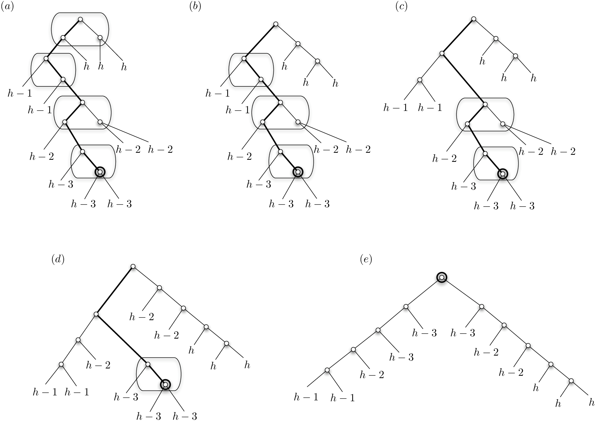
Let $x$ be the deepest nodes on the top path of $A$ , such that the unmarked child of $x$ corresponds to the root of the bottom tree $A^{\prime}$ . The extraction process will separate the nodes of depth (in $P$ ) smaller than $d=d_{P}(x)+\log\log n$ from the bottom tree $A^{\prime}$ . Let a zig segment of a preferred path $p$ be a maximal sequence of nodes such that each node in the sequence is linked to its right child in $p$ . A zag segment is defined similarly such that each node on the segment is linked to its left child (see Fig. 2).

The key observation we exploit is the following: the sequence of all zig segments, ordered by their depth in the path, followed by the sequence of all reversed zag segments, ordered reversely by their depth in the path, is equal to the ordering of the nodes in key space (see Fig. 2). This implies that to extract the nodes of depth smaller than $d$ (in $P$ ) from a bottom tree, we can cut the extreme ends (in key space) of the tree, linearize them to two lists, and then combine them by a binary merge procedure using depth in $P$ as the ordering. This forms the core of the extract operation.

We have to do this using rotations, while maintaining a tree at all times. We now give the details of how to do this, with Fig. 3 illustrating the process.

Using extra fields of each node storing the minimum and maximum depth value (in $P$ ) of nodes inside its subtree, we can find the node $\ell^{\prime}$ of minimum key value that has a depth greater than $d$ in $O(\log\log n)$ time, by starting at the root of $A^{\prime}$ and repeatedly walking to the leftmost child whose subtree has a node of depth greater than $d$ . Then define $\ell$ as the predecessor of $\ell^{\prime}$ . Symmetrically, we can find the node $r^{\prime}$ of maximum key value that has depth greater than $d$ and define $r$ as the successor of $r^{\prime}$ .

First we split $A^{\prime}$ at $\ell$ to obtain two subtrees $B$ and $C$ linked to the new root $\ell$ where $B$ contains a first sequence of nodes at depth smaller than $d$ . Then we split $C$ at $r$ to obtain the subtrees $D$ and $E$ where $E$ contains a second sequence of nodes at depth smaller than $d$ .

In $O(\log\log n)$ time we convert the subtrees $B$ and $E$ into paths corresponding to an ordered sequences of zig segments for $B$ and zag segments for $E$ . To do so we perform a left rotation at the root of $B$ until its right subtree is a leaf (i.e., when its right child is a marked node). Then we repeat the following: if the left child of the root has no right child the we perform a right rotation at the root of $B$ (adding one more node to right spine, which will constitute the final path). Otherwise we perform a left rotation at the left child of the root of $B$ , moving its right subtree into the left spine. This process takes a time linear in the size of $B$ , since each node is involved in a rotation at most 3 times (once a node enters the left spine, it can only leave it by being added to the right spine). A symmetric process is performed to convert the subtree $E$ into a path.

The last operation, called a zip, merges (in term of depths in $P$ ) the two paths $B$ and $E$ , in order to form the next part of the top path. We repeatedly select the root of $B$ or $E$ that has the smallest depth in the tree $P$ . The selected root is brought to the bottom of the top path using $O(1)$ rotations. The zip operation stops when the subtrees $B$ and $E$ are both empty. Eventually, we perform a left rotation at the node $\ell$ if needed, i.e., if $r$ has a smaller depth in $P$ than $\ell$ .

The time taken is linear in the extracted number of nodes, i.e, $\log\log n$ . The process consists of a series of rotations, hence can stopped and resumed without problems.

Therefore, the discussion presented in this section allows us to conclude with the following theorem.

Theorem 2

Our hybrid tree data structure is $O(\log\log n)$ -competitive and performs each access in $O(\log n)$ worst-case time.

3.3 Hybrid Trees and the BST Model

We specify in the description of the cut operation (more precisely, in case 1) that the extraction process is executed incrementally, i.e., the work is spread over several cut operations. In order to efficiently revive an extraction process which has been stopped at some point in the past, we have to return to the position where its next rotation should take place. This location is unique for each path representation, and is always in its bottom tree. Thus, traversing its top path to reach the bottom tree would be too costly for the analysis of case 1. Instead, we store in the marked node (the first node of the top path) appropriate information on the state of the process. Additionally, we store an extra pointer pointing to the node where the next rotation in the process should take place. This allows us to revive an extraction process in constant time. Unfortunately, the structure so obtained is not in the BST model (see Section 2.1), due to the extra pointer. In the next section we show how to further develop the idea from this section into a data structure fitting the BST model.

Still, we note that the structure of this section can be implemented in the comparison based model on a pointer machine, with access sequences $X$ being served in $O(\log\log n\,{\rm OPT}(X))$ time, and each access taking $O(\log n)$ time worst-case.

4 Zipper Trees

The data structure described in the previous section is a BST, except that each marked node has an extra pointer facilitating constant time access to the point in the path representation where an extraction process should be revived. In this section, we show how to get rid of this extra pointer and obtain a data structure with the same complexity bounds, but now fitting the BST model described in Section 2.1. To do so, we develop a more involved version of the representation of preferred paths and the operations on them. The goal of this new path representation is to ensure that all rotations of an extraction process are located within distance $O(1)$ of the root of the tree of the representation. The two main ideas involved are: 1) storing the top path as lists, hanging to the sides of the root, from which the top path can be generated incrementally by merging as it is traversed during access, and 2) using a version of the split operations that only does rotations near the root. The time complexity analysis follows that of hybrid trees, and will not be repeated.

4.1 Path Representation

For all preferred paths in $P$ we decompose its highest part into two sequences, containing its zig and its zag segments, respectively. These are stored as two paths of nodes, of increasing and decreasing key values, respectively. As seen in Section 3.2 (cf. Fig. 2), both will be ordered by their depth in $P$ . Let $\ell$ and $r$ be the highest node in the zig and zag sequence respectively. The node $\ell$ will be the root of the auxiliary tree (the marked node). The remainder of the zig sequence is the left subtree of $\ell$ , $r$ is its right child, and the remainder of the zag sequence is the right subtree of $r$ . We call this upper part of the tree a zipper. We repeat this decomposition once again for the next part of the path to obtain another zipper which is the left subtree of $r$ . Finally the remaining of the nodes on the path are stored as a red-black tree of height $O(\log\log n)$ , hanging below the lowest zipper. Fig. 4 illustrates the construction. The two zippers constitute the top path, and the red-black tree the bottom tree. Note that the root of the bottom tree is reachable in $O(1)$ time from the root of the path representation. We will maintain the invariant that individually, the two zippers contain at most $\log\log n$ nodes each, while (if the bottom treeis non-empty) they combined contain at least $(\log\log n)/2$ nodes.

A zipper tree consists of all the preferred paths of $P$ , represented as above, linked together to form one large tree.

4.2 Maintaining Zipper Trees under Accesses

We now give the differences, relative to Section 3.2, of the operations during an access.

CUT:

When searching a path representation, we incrementally perform a zip operation (i.e., a merge based on depth order) on the top zipper, until it outputs either the node searched for, or a node that leads to the next path representation. If the top zipper gets exhausted, the lower zipper becomes the upper zipper, and an incremental creation of a new lower zipper by an extraction operation on the bottom tree is initiated (during which the lower zipper is defined to have size zero). Each time one more node from the top zipper is being output (during the current access, or during a later access passing through this path representation), the extraction advances $\Theta(1)$ steps. The speed of the extraction process is chosen such that it finishes with $\log\log n$ nodes extracted before $(\log\log n)/2$ nodes have been output from the top zipper. The new nodes will make up a fresh lower zipper, thereby maintaining the invariant.

If the access through a path representation overlaps (in time) at most one extraction process (either initiated by itself or by a previous access), it is defined as a case 1 cut. No further actions takes place, besides the proper remarkings of roots of path representations, as in Section 3.2. If a second extraction process is about to be initiated during an access, we know that $\Theta(\log\log n)$ nodes have been passed in this path representation, and we define it as a case 2 cut. Like in Section 3.2 this now ends by converting the path representation to a red-black tree, cutting it like in tango trees, and then converting the red-black tree remaining into a valid path representation (as defined in the current section), all in $\Theta(\log\log n)$ time.

CONCATENATE:

There is no change from Section 3.2, except that the final path representation produced is as defined in the current section.

EXTRACT:

The change from Section 3.2 is that the final zip operation is not performed (the process stops at step (d) in Fig. 3), and that we must use a search and a split operation on red-black trees where all structural changes consist of rotations a distance $O(1)$ from the root²² 2 As no actual details of the split operation used are given in [2], we do not know whether their split operation fulfills this requirement. It is crucial for our construction that such a split operation is possible, so we describe one solution here. (of the bottom tree, which is itself at a distance $O(1)$ from the root of the zipper tree). Such a split operation is described in the appendix (Part I). Note that searching takes place incrementally as part of the split procedure.

5 Conclusion

The main goal in this area of research is to improve the competitive ratio of $O(\log\log n)$ . Here we have been able to tighten other bounds, namely the worst-case search time. We think this result helps providing a better understanding of competitive BSTs. It could be that competitiveness is in conflict with balance maintenance, i.e., an $O(1)$ -competitive binary search tree could possibly not guarantee an $O(\log n)$ worst-case search time. For instance splay-tree [10] and GreedyFuture tree [9, 3], the two BSTs that are conjectured to be dynamically optimal, do not guarantee optimal worst-case search time. Thus even if dynamically optimal trees exist, our result could still be a good alternative with optimal worst-case performance.

We also think that the ideas developed to achieve our result have their own interest. They can be used to improve the worst-case performance of a data structure while maintaining the same amortized performance. For example we show in the appendix (Part II) how to adapt them in order to improve the worst-case running time of the multipop operation on a stack.

References

[1] T. H. Cormen, C. E. Leiserson, R. L. Rivest, and C. Stein. Introduction to Algorithms. MIT Press, 2001. Section 10.1: Stacks and queues, pages 200–204.
[2] E. Demaine, D. Harmon, J. Iacono, and M. Pătraşcu. Dynamic optimality—almost. SICOMP, 37(1):240–251, 2007. Also in Proc. FOCS 2004.
[3] E. D. Demaine, D. Harmon, J. Iacono, D. M. Kane, and M. Patrascu. The geometry of binary search trees. In Proc. of the 10th ACM-SIAM Symp. on Disc. Alg. (SODA), pages 496–505, 2009.
[4] J. Derryberry, D. D. Sleator, and C. C. Wang. ${O}(\log\log n)$ -competitive dynamic binary search trees. In Proc. of the 7th ACM-SIAM Symp. on Disc. Alg. (SODA), pages 374–383, 2006.
[5] G. F. Georgakopoulos. Chain-splay trees, or, how to achieve and prove loglogn-competitiveness by splaying. Inf. Process. Lett., 106(1):37–43, 2008.
[6] L. J. Guibas and R. Sedgewick. A dichromatic framework for balanced trees. In Proc. of the 19th Found. of Comp. Sci. (FOCS), pages 8–21, 1978.
[7] J. Iacono. Personal communication, July 2009.
[8] J. Kujala and T. Elomaa. Poketree: A dynamically competitive data structure with good worst-case performance. In Proc. ISAAC 2006, volume 4288 of LNCS, pages 277–288, 2006.
[9] J. I. Munro. On the competitiveness of linear search. In Proc. of the 8th Annual European Symposium (ESA), volume 1879 of LNCS, pages 338–345, 2000.
[10] D. D. Sleator and R. E. Tarjan. Self-adjusting binary search trees. J. ACM, 32(3):652–686, 1985.
[11] C. C. Wang. Multi-Splay Trees. PhD thesis, Computer Science Department, School of Computer Science, Carnegie Mellon University, 2006.
[12] R. Wilber. Lower bounds for accessing binary search trees with rotations. SICOMP, 18(1):56–67, 1989.
[13] S. L. Woo. Heterogeneous Decomposition of Degree-Balanced Search Trees and Its Applications. PhD thesis, Computer Science Department, School of Computer Science, Carnegie Mellon University, 2009.

APPENDIX

Part I

We present the split operation on red-black trees where all structural changes consist of rotations a distance $O(1)$ from the root.The end result should be a tree where the root is the node $x$ split on, with a left child that is a red-black tree on the nodes smaller than $x$ , and a right child that is a red-black tree on the nodes larger than $x$ . Red-black trees are binarized (2,4)-trees, i.e., multi-way nodes are substituted by small, perfectly balanced binary search trees, with the color annotation keeping track of the boundaries between them. For ease of exposition, we describe the split process partly in (2,4)-tree terms.

The overall idea of a normal split operation on (2,4)-trees is to follow the search path towards $x$ and cleave (2,4)-tree nodes passed, then later glue the two parts of cleaved nodes (now maybe of too low degree) to their level-wise siblings (now maybe of too high degree), and then split (in the sense of rebalancing of (2,4)-nodes) these if necessary. By cleaving a (2,4)-node, we mean dividing the keys (here, binary nodes) inside the (2,4)-node, and the subtrees of the (2,4)-node, into two parts, based on whether they order-wise are smaller or larger than $x$ .

Normally, cleaving is top-down, and gluing and splitting is bottom-up. However, to keep the working point, where the rotations take place, fixed at the root—and maintain a BST at all times—we instead fold the two sides of the cleaved path around during searching-and-cleaving (treating each side of the cleaved path sort of as a rope in a pulley, the pulleys being the working point), while keeping track of heights (in (2,4)-tree terms) of subtrees. Later, the gluing process is done in a reverse action (running the ropes the other way), while making use of the heights of subtrees.

We now describe the details of the cleaving process. We assume wlog. that the search path initially proceeds to the left child of the root (the other case being symmetric). During the cleaving process, we maintain the following shape of the binary tree: Let $P$ be the search path of the initial red-black tree traversed so far, and let $P_{(2,4)}$ be the (2,4)-nodes touched by $P$ . The top of the right spine (including the root) consists of the binary nodes in $P_{(2,4)}$ whose keys are larger than $x$ . The subtrees hanging from these nodes are the subtrees of $P_{(2,4)}$ which are larger than $x$ . The top of the left spine (excluding the root) consists of the binary nodes in $P_{(2,4)}$ whose keys are smaller than $x$ . The subtrees hanging from these nodes are the subtrees of $P_{(2,4)}$ which are smaller than $x$ , except for the topmost of the subtrees, which is the remaining part of the initial tree. See Fig. 5.

Advancing the cleaving process by one more (2,4)-node of the search path means rebuilding a subtree consisting of at most the root, its left child, and the up to three binary nodes of the next (2,4)-node. This rebuilding can be done in $O(1)$ rotations on these nodes. The cleaving process ends when the (2,4)-node containing $x$ is the next such node, with a final rebuilding which brings $x$ up as root.

We now need to change both subtrees of the root into valid red-black trees. This will be done in a downwards fashion, one spine at a time. We describe the process for one spine.

The heights, as (2,4)-trees, of the subtrees hanging from the top of the spine are increasing when going downwards. There are initially between zero and three subtrees of each height. For sake of induction, we assume there are between zero and five subtrees of each height. If there are at least two subtrees of the next height $h$ , one or two (2,4)-nodes of height $h+1$ , hanging from the spine, are formed by rotations on the top nodes of the spine. These nodes will take part in the next group of (2,4)-nodes of heights $h+1$ , and the process continues with these. Otherwise, there is at most one subtree of height $h$ , and we will look to the next non-empty group of subtrees (of height $h+k$ for some $k>0$ ) hanging from the spine. Of these subtrees, all valid (2,4)-trees, we fold the top-most one around its root: the binary nodes in its (2,4)-tree root are moved onto the spine using rotations, making its (2,4)-tree subtrees hang from the spine. This is repeated $k$ times, which leaves hanging from the spine between one and three new subtrees of height $h+k-i$ , for $i=1\dots k-1$ , and between two and four new subtrees of height $h$ , at the cost of $O(k)$ rotations. There are now at least two subtrees of height $h$ hanging from the spine, and the process continues with these. By induction, there will never be more than five trees of any size during this process, and we will end up with a legal (2,4)-tree, hence a legal red-black tree.

The total time of the split is bounded by the height of the initial tree.

Part II: Stack with Improved Multipop Operation

A stack [1] is a fundamental data structure that asks for the following operations:

•

PUSH( $x$ ) – insert the element $x$ on the top of the stack.
•

POP() – delete the element from the top of the stack if it is not empty.
•

MULTIPOP( $k$ ) – deletes $k$ elements from the top of the stack, or deletes all elements if the stack has less than $k$ elements.

In a pointer machine, a stack is usually implemented as a simple linked list. The operation PUSH( $x$ ) creates an element with value $x$ and insert it as the new head of the list. The operation POP() removes the head of the list if this one is not empty. The operation MULTIPOP( $k$ ) is performed using $k$ times the POP() operation.

Over a sequence of stack operations the amortized cost of each operation is $O(1)$ since an element that has been pushed on the stack can only be popped once from it. Concerning the worst-case performance of the operations it is clear that PUSH( $x$ ) and POP() take O(1) wost-case time whereas MULTIPOP( $k$ ) takes $O(k)$ worst-case time. Thus the worst-case running time of this operation can reach $O(n)$ if $k\geq n$ where $n$ is the number of elements in the stack. Here we develop a stack that improves the running time of MULTIPOP().

The structure is composed of two parts: first a linked list $L$ of size $\Theta(\log n)$ that contains the most recently pushed elements (as in the original structure) and secondly a red-black tree [6] $T$ containing the remaining elements. Each element $x$ in the stack has a height $h(x)$ which is defined as the number of elements that were in the stack before $x$ was pushed in. The tree $T$ is ordered based on the height of the elements so that the elements in the left (or the right) subtree of an element $x$ have a smaller (or greater) height than $h(x)$ . The size $|T|$ of the tree is stored at its root.

The stack operations PUSH( $x$ ) and POP() (MULTIPOP() is considered later) are essentially performed as in the standard structure. They either add a new head element to the list $L$ or remove it. Thus $L$ is modified and the invariant about its size has to be maintained, i.e., $|L|=\Theta(\log n)$ . More specifically we maintain $\log n\leq|L|\leq 5\log n$ . In order to do so we use an extraction and a contraction process, described below, which transfer $\log n$ elements from the tree into the list or from the list into the tree, respectively, in $O(\log n)$ steps. These processes run incrementally: Whenever an element is popped/pushed from the list, the ongoing extraction/contraction process is advanced by $\Theta(1)$ steps and then the process is suspended until the next operation occurs. Thus the work of an extraction/contraction process is spread over several operations (if not stopped before by a specific kind of MULTIPOP() operation, see below) which means that PUSH( $x$ ) and POP() still take $O(1)$ worst-case time. The speed of the process is chosen such that the extraction/contraction of $\log n$ elements is completed before $\log n$ push/pop operations have been performed. Whenever $|L|$ reaches $4\log n$ a contraction process is launched and when $|L|$ reaches $2\log n$ an extraction process is launched. Hence there is no more than one extraction/contraction process running at the same time and the size of the list is always maintained between $\log n$ and $5\log n$ .

The operation MULTIPOP(k) is performed in the following way: if $k\leq\log n$ then we perform $k$ times the POP() operation which takes $O(k)$ worst-case time. Otherwise we finish any pending extraction/contraction process in the stack. We perform $O(1)$ contraction processes until all the elements are contained in the tree $T$ . Then we binary search in $T$ for the element $x$ with $h(x)=|T|-k$ and we perform a cut of the tree at the element $x$ using the standard cut operation of red-black trees [6]. The tree containing the $k$ highest elements of the stack is discarded. Finally we perform three extraction processes so that the stack satisfies the invariant. This takes $O(\log n)$ worst-case time in total.

We present the extraction and the contraction process mentioned in the previous description:

EXTRACT() is the operation that transfers the $\log n$ highest elements from the red-black tree into the linked list in $O(\log n)$ time. It first binary searches in $T$ the element $x$ with $h(x)=|T|-\log n$ . Once $x$ is found, the tree $T$ is split at $x$ using the standard split operation of red-black trees [6]. The extracted tree containing the highest elements is converted in a linked list in $O(\log n)$ time and finally attached to the end of the list of the stack.

CONTRACT() is the operation that performs the inverse of EXTRACT() with the same running time. It transfers the set $S$ of the $\log n$ lowest elements from the linked list into the red-black tree in $O(\log n)$ time. The operation performs a walk along the list to find the position of the first element of $S$ , then the list is cut at this precise point. The sublist containing the elements of $S$ is converted into a red-black tree in $O(|S|)=O(\log n)$ time. Finally the newly obtained tree is joined, in $O(\log n)$ , with the red-black tree of the stack.

Theorem 3

A stack can be implemented such that the operations PUSH() and POP() take $O(1)$ wost-case time and the operation MULTIPOP( $k$ ) takes $O(\min\{k,\log n\})$ worst-case time. All these operations take $O(1)$ amortized time.

An O⁡(log⁡log⁡n)O(\log\log n)-Competitive Binary Search Tree with Optimal Worst-Case Access Times

Abstract

1 Introduction

2 Preliminaries

2.1 BST Model

2.2 Interleave Lower Bound

Theorem 1

2.3 Tango Trees

3 Hybrid Trees

3.1 Path Representation

Lemma 1

3.2 Maintaining Hybrid Trees under Accesses

CUT:

CONCATENATE:

EXTRACT:

Theorem 2

3.3 Hybrid Trees and the BST Model

4 Zipper Trees

4.1 Path Representation

4.2 Maintaining Zipper Trees under Accesses

CUT:

CONCATENATE:

EXTRACT:

5 Conclusion

References

APPENDIX

Part I

Part II: Stack with Improved Multipop Operation

Theorem 3

An $O(\log\log n)$ -Competitive Binary Search Tree with Optimal Worst-Case Access Times