Quantum Bose Josephson Junction with binary mixtures of BECs
Abstract
We study the quantum behaviour of a binary mixture of Bose-Einstein condensates (BEC) in a double-well potential starting from a two-mode Bose-Hubbard Hamiltonian. We focus on the small tunneling amplitude regime and apply perturbation theory up to second order. Analytical expressions for the energy eigenvalues and eigenstates are obtained. Then the quantum evolution of the number difference of bosons between the two potential wells is fully investigated for two different initial conditions: completely localized states and coherent spin states. In the first case both the short and the long time dynamics is studied and a rich behaviour is found, ranging from small amplitude oscillations and collapses and revivals to coherent tunneling. In the second case the short-time scale evolution of number difference is determined and a more irregular dynamics is evidenced. Finally, the formation of Schroedinger cat states is considered and shown to affect the momentum distribution.
pacs
03.75.Lm, 67.85.Fg, 74.50.+rI Introduction
The experimental discovery of Bose-Einstein condensation [1] in dilute systems of trapped alkali-metal atoms, such as rubidium (), lithium (), sodium () and ytterbium (), has spurred a renewed interest into the investigation of macroscopic quantum phenomena and interference effects, allowing for a deeper understanding of the conceptual foundations of quantum mechanics [2]. This fascinating research area has been growing up thanks to the high degree of experimental manipulation and control [3]. Interference between condensates released in a potential with a barrier was first observed in 1997 [4] and that paved the way for further investigations on the problem of Bose condensates in a double well potential. Then Josephson oscillations have been observed in one dimensional optical potential arrays [5]. A single bosonic Josephson junction was produced for the first time in 2005 with atoms and its dynamics was experimentally investigated both within tunneling as well as self-trapping regime [6][7][8]. More recently, mixtures of and atoms have been produced and experimentally investigated [9] as well, whose intraspecies scattering lengths could be tunable via magnetic and optical Feshbach resonances. Furthermore the realization of heteronuclear mixtures of and atoms with tunable interspecies interactions [10] paved the way to the exploration of double species Mott insulators and, in general, of the quantum phase diagram of two species Bose-Hubbard model [11]. The interplay between the interspecies and intraspecies scattering produces deep consequences on the properties of the condensates, such as the density profile [12] and the collective excitations [13]. However, the wide tunability of such interactions makes a BEC mixture a very interesting subject of investigation, both from experimental and theoretical side as a mean of studying new macroscopic quantum tunneling phenomena as well as the interplay between quantum coherence and nonlinearity. Indeed novel and richer behaviours are expected in such a multicomponent BEC.
On the theoretical side, a bosonic Josephson junction with a single species of BEC has been widely investigated by means of a two-mode approximation [14][15][16], within the classical as well as the quantum regime. In the classical regime, characterized by large particle numbers and weak repulsive interactions, the Gross-Pitaevskii equation provides a reliable description. Within the two mode approximation it reduces to two generalized Josephson equations which describe the time evolution of the relative phase and the population imbalance between the wells [15] and differ from their superconducting counterpart [17] by the presence of a nonlinear term which couples the variables. Because of such a term, a bosonic Josephson junction exhibit a variety of novel phenomena which range from -oscillations to macroscopic quantum self-trapping (MQST) [15]. While the -oscillations, as well the usual Josephosn ones, deal with a symmetric oscillation of the condensate about the two wells, the MQST phenomenon is characterized by a broken symmetry phase with a population imbalance between the wells. In the quantum regime, characterized by smaller values of the particle number and strong interactions, an increasing of phase fluctuations is observed together with the suppression of number fluctuations. Furthermore the time evolution is characterized by phase collapse and revival [18]. The quantum behaviour of bosonic Josephson junctions has been deeply investigated by means of the usual quantum phase model [19][20][21] as well as by starting from a two-mode Bose-Hubbard Hamiltonian [22][23][24]. In this context the phase coherence of the junction has been characterized by studying the momentum distribution [25][20]. The generation and detection of Schroedinger cat states has been investigated as well; indeed the presence of such a kind of states reflects in the strong reduction of the momentum-distribution contrast [24][26].
More recently such a theoretical analysis has been successfully extended to a binary mixture of BECs in a double well potential [27][28] [29][30]. The semiclassical regime in which the fluctuations around the mean values are small has been deeply investigated and found to be described by two coupled Gross-Pitaevskii equations. By means of a two-mode approximation such equations can be cast in the form of four coupled nonlinear ordinary differential equations for the population imbalance and the relative phase of each species. The solution results in a richer tunneling dynamics. In particular, two different MQST states with broken symmetry have been found [29], where the two species localize in the two different wells giving rise to a phase separation or coexist in the same well respectively. Indeed, upon a variation of some parameters or initial conditions, the phase-separated MQST states evolve towards a symmetry-restoring phase where the two components swap places between the two wells, so avoiding each other. Recently, the coherent dynamics of a two species BEC in a double well has been analyzed as well focussing on the case where the two species are two hyperfine states of the same alkali metal [31].
In this paper we study the quantum behaviour of a binary mixture of Bose-Einstein condensates (BEC) in a double-well potential starting from a two-mode Bose-Hubbard Hamiltonian. We analyze in detail the small tunneling amplitude regime where number fluctuations are suppressed and a Mott-insulator behaviour is established. We perform a perturbative calculation up to second order in the tunneling amplitude and study the stationary states and the dynamics of the two species bosonic Josephson junction. Finally, the dynamical generation of Schroedinger cat states is investigated starting from an initial coherent spin state and shown to affect the time-dependent population imbalance and momentum distribution[25][20]. We focus on the contrast in the momentum distribution between the two wells and show how it vanishes for a two-component cat state. That could be interesting in view of the experimental realization of macroscopic superpositions of quantum states [26][32].
The paper is organized as follows. In Section 2 we introduce our model Hamiltonian within the two-mode approximation and define the various parameters. Then we adopt the angular momentum representation and focus on the small tunneling amplitude regime. In Section 3 we apply perturbation theory in the tunneling amplitude to our Hamiltonian and find analytical expressions for the energy eigenvalues and eigenstates up to second order. Section 4 and 5 are devoted to the study of the quantum evolution of the number difference of bosons between the two wells in correspondence of two different initial conditions: completely localized states and coherent spin states. In the first case both the short and the long time dynamics is studied and a rich behaviour is evidenced, ranging from small amplitude oscillations and collapses and revivals to coherent tunneling. In the second case the short-time scale evolution of number difference is determined and a more irregular dynamics is evidenced, with suppression of the dominant frequency when the number of bosons increase. Then, Schroedinger cat states are shown to generate as a result of the time-evolution of an initial coherent state when the tunneling between the two wells is suppressed, and their influence on the contrast in the momentum distribution is studied. Finally, in Section 6 some conclusions and outlooks of this work are presented.
II The model
A binary mixture of Bose-Einstein condensates [28][29] loaded in a double-well potential is described by the general many-body Hamiltonian:
| (1) |
where
| (2) |
| (3) |
are the Hamiltonians for bosons of species and respectively and
| (4) |
is the interaction term between bosons of different species. For dilute mixtures one can replace the interaction potentials , and with the effective contact interactions:
| (5) |
where and are the intraspecies coupling constants of the species and respectively, and being the atomic masses and , the -wave scattering lengths; furthermore is the interspecies coupling constant, where is the reduced mass and is the associated -wave scattering length. In this way the Hamiltonian (1)-(4) can be rewritten as:
| (6) |
| (7) |
Here is the double well trapping potential and, in the following, we assume ; , are the bosonic creation and annihilation operators for the two species, which satisfy the commutation rules:
| (8) | |||||
| (9) |
and the normalization conditions:
| (10) |
, being the number of atoms of species and respectively. The total number of atoms of the mixture is .
Now a weak link between the two wells produces a small energy splitting between the mean-field ground state and the first excited state of the double well potential and that allows us to reduce the dimension of the Hilbert space of the initial many-body problem. Indeed for low energy excitations and low temperatures it is possible to consider only such two states and neglect the contribution from the higher ones, the so called two-mode approximation [14] [15][16]. In this way, by taking into account for each of the two species and the mean-field ground states , and the mean-field excited states , , the wave functions , , can be rewritten as:
| (11) |
where , , and , and , (, and , ) are the creation (annihilation) operators for a particle of the species , in the ground and the excited state respectively. They satisfy the usual bosonic commutation relations . Furthermore , are assumed real for simplicity and such that , which simplifies the calculations. Let us change the basis and switch to the atom number states in such a way that the expectation value of the population of the left and right well can be defined. The new annihilation operators are , and , for the species and respectively, so that the wave functions (11) become:
| (12) |
By substituting Equations (12) into the Hamiltonian (6)-(7), after some algebra we obtain its second quantized version within the two-mode approximation:
| (13) | |||||
where , , is the number of atoms of species and respectively, expressed as a sum of numbers of atoms in the left and right well. The parameters are defined as follows:
| (14) |
| (15) |
| (16) |
| (17) |
| (18) |
| (19) |
| (20) |
| (21) |
| (22) |
In Eq. (13), the terms proportional to , , describe tunneling of particles of species and from one to the other well while the terms proportional to , , deal with the local interaction within the two wells and the terms proportional to correspond to additional two-particle processes. Finally the terms proportional to and couple the two species and then various constant terms follow, which we will drop for simplicity.
In this paper we focus on the small tunneling amplitude regime where number fluctuations are suppressed and a Mott-insulator behaviour is established, so it is convenient to introduce the angular momentum representation for the species and as follows:
| (23) |
where the operators , , , obey to the usual angular momentum algebra and the following relations hold:
| (24) |
In particular, the components , give the difference of the number of bosons of the species , and , occupying the two minima of the double well potential, i. e. the population imbalances, which are experimentally observable quantities. Thus Hamiltonian (13) can be cast in the following form:
| (25) | |||||
where the constant terms have been dropped. Let us now simplify the notation by introducing the following parameters:
| (26) |
and rewrite the Hamiltonian (25) as:
| (27) | |||||
Within the experimental parameters range it is possible to show that , , and [7][29], then in the following we put and , which corresponds to neglecting the spatial overlap integrals between the localized modes in the two wells. In this way the binary mixture of BECs within two-mode approximation maps to two Ising-type spin model in a transverse magnetic field.
In the following we will focus on the symmetric case and because it allows us to perform analytical calculations while capturing many relevant phenomena characterizing the physics of the system. So the model Hamiltonian (25) becomes:
| (28) |
| (29) |
| (30) |
where, in the small tunneling amplitude regime, is considered as a perturbation. The total Hamiltonian commutes with and , which leads to the conservation of total angular momentum with quantum numbers and respectively. So the whole Hilbert space has finite dimension, equal to , thus it depends on the number of bosons of the species and respectively. The whole basis is given by the eigenvectors of () and () with and .
As a first step we need to diagonalize the unperturbed Hamiltonian (29), which can be done by performing the following rotation on the operators , :
| (31) |
while an analogous rotation needs to be carried out on , entering the perturbation (30). As a result we get:
| (32) |
which, by defining , , and , , , , can be cast in the final form:
| (33) |
In the following Section we will find analytical expressions for the eigenvalues and the eigenvectors up to second order by performing perturbation theory in the tunneling amplitude.
III Stationary states
In the present Section we apply second-order perturbation theory to the Hamiltonian of Eq. (33) in the small tunneling amplitude limit, which allows us to derive analytical expressions for the stationary states of the system.
In order to pursue this task let us rewrite Eq. (33) in dimensionless form by assuming as unit of energy:
| (34) |
where and , then take
| (35) |
as unperturbed Hamiltonian and
| (36) |
as a small perturbation term. Here , , obey the usual angular momentum algebra and the following relation holds:
| (37) |
where:
| (38) |
In principle, the rotated basis of the unperturbed Hamiltonian (35) is given by the eigenvectors of () and () with and , whose corresponding eigenvalues are .
The presence of the operator , which does not commute with the perturbation term , makes the problem of finding eigenvalues and eigenvectors of the full Hamiltonian (34) within perturbation theory much more involved. In order to simplify the treatment and carry out analytical calculations while retaining the relevant phenomenology, we concentrate on the particular case of a binary mixture where the two species are equally populated, i. e. , and have the same population imbalance between the two wells, i. e. . This situation allows us to describe the quantum dynamics of the system in correspondence of the MQST regime, for which we need a completely localized initial state. That fixes while could be an even or odd integer depending on even or odd, and leads to the following zero-order eigenvalues: . Each eigenvalue is two-fold degenerate, with the only exception of the ground state for even, , which is nondegenerate. The two-dimensional subspace of degeneracy is spanned by the states (where ) and the corresponding zero-order eigenvectors are:
| (39) |
By switching on the perturbation term (36) it is possible to show that the degeneration is lifted starting from the levels with smaller ; in general the double degeneracy of the zero-order eigenvalues will be lifted at the -th order of perturbation theory [22]. By applying perturbation theory [33] up to order , we obtain the following corrected eigenvalues:
| (40) |
| (41) |
| (42) |
where . Furthermore, for even, the nondegenerate ground state belongs to the symmetry class of . The corresponding eigenvectors, up to order , are given in the Appendix.
IV Dynamics: completely localized initial states
In this Section we investigate the quantum evolution of the number difference of bosons of species and between the two wells assuming a completely localized state as initial condition. That could be interesting in order to elucidate the quantum behavior of the system in correspondence of the classical MQST regime and to put in evidence new phenomena including quantum coherence in a multicomponent system. In such a case we will study both the short and the long time dynamics: as a result a rich behaviour emerges, ranging from small amplitude oscillations and collapses and revivals to coherent tunneling. Although such a physics is well known for the single component Bose Josephson junction, in our case the dynamics shows that the two species can coexist in the same potential well as if there would be an attractive interaction between them.
As a first step let us recall the general formula which gives the time evolution of the mean value of [33]:
| (43) |
where is the dimensionless time, the sums are over all the eigenvectors , being or , and are the projections of the initial state on the basis :
| (44) |
So it is clear how the knowledge of eigenvalues and eigenvectors is enough in order to study the quantum evolution of , the Bohr frequencies involved, , and the corresponding weights .
Let us now study the dynamics of the system when all the bosons of species and are initially contained in one of the two wells of the potential, say the right one, and then the imbalances of the two species coincide, so that , , , ; furthermore the two species are equally populated, i.e. . That implies and in our center of mass rotated basis. The corresponding initial condition is:
| (45) |
In order to investigate the short timescales evolution we need to keep terms up to second order in the tunneling amplitude when we compute the weights in Eq. (43). We find that:
| (46) |
where the frequency involved is:
| (47) |
At short timescales small amplitude oscillations with frequency around the initial condition (, ) are observed and that coincides with a strongly self-trapped regime.
In order to investigate the dynamics at longer timescales we have to take into account also the small splittings and of the two higher pairs of quasidegenerate eigenvalues which provide two further frequencies (see Ref. [23] for the derivation):
| (48) |
The whole result is:
| (49) | |||||
and, by putting , the short timescale dynamics, Eq. (46), is recovered. Summarizing, at longer timescales the two species bosons are still localized in the initial potential well but the quantum dynamics exhibits collapses and complete revivals. Indeed the coefficient , which multiplies the higher frequency term , gives rise to the beat, which is responsible for the observed collapses and revivals at timescales fixed by , as shown in Fig. 1. Finally, at very large timescales determined by the frequency all the bosons tunnel coherently back and forth between the two traps; only the first term is responsible of such a coherent tunneling, since all harmonic functions containing the frequency and are small in amplitude and proportional to , thus they are unable to transfer bosons from one trap to the other.
The tunneling dynamics within macroscopic quantum self-trapping regime described above is analogous to that of the -mode fixed point obtained by the Gross-Pitaevski approach [29], where the two species localize in the same well despite the repulsive interaction between them. Let us finally note that, despite the explicit dependence on of the frequencies (47)-(48), the different physics related to the three time scales described above is simply due to the energy splitting introduced by the renormalized tunneling for small . Thus in the case of a mixture of BECs with equal population the dynamics remains similar to that of a single component BEC, apart the coexistence of the two species in the same well.
As for the experimental detection of the long timescales phenomena (collapses/revivals and coherent tunneling), since the time for their appearance is abruptly increased with , this implies a rapid decrease of the characteristic frequencies rendering more difficult the observation of the intermediate and long time behavior in current BEC experiments. Indeed pure condensates consisting of atoms of loaded in a double well have been recently realized [6][7] thus rendering the detection of the intermediate time behavior possible. Mixtures with a number of atoms ranging from and ( and [9]) to and ( and [10]) have also been recently realized, but in this case very small characteristic frequencies are implied. However, these phenomena may be relevant for molecular systems where the number of vibrational excited quanta is small.


In the next Section we will further investigate the dynamics of the system by assuming as initial state a simple coherent state and then study the formation of a particular superposition of such coherent states, the so called Schroedinger cat states.
V Dynamics: coherent spin initial states and Schroedinger cat states
In this Section we choose as initial condition a simple coherent spin state [34] and study the short-time scale evolution of number difference; in this way a more complex dynamics will appear. Finally, we study the generation of Schroedinger cat states; in particular, we focus on the contrast in the momentum distribution and show how it vanishes for a two-component cat state.
Let us start by considering as initial condition the following coherent spin state [34]:
| (50) |
where the coefficient is:
| (51) |
and and are two angles characterizing the superposition. The time evolution of the mean value of up to first order in the tunneling amplitude is given by:
| (52) | |||||
where
| (53) |
with frequencies . Furthermore the coefficients and are given by:
| (54) |
| (55) |
for even, and
| (56) |
| (57) |
for odd, respectively. Finally, for even, the zero-order mean value is given by:
| (58) | |||||
where the dominant frequency is equal to . The corresponding expression for odd is:
| (59) | |||||
where . As one can see, the dominant frequency is gradually suppressed with the number of bosons [22]. This
is clearly seen in Fig. 2 where the boson number
difference between the two traps is plotted for different (even)
values as a function of the dimensionless time . One also notices a decrease of the oscillation amplitude at
increasing .
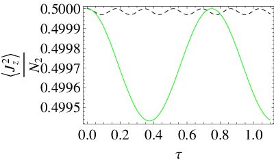
The effect of is instead shown in Fig. 3
where the short-time dynamics of the boson number difference is analyzed for
two values of the interspecies interaction. When increases the
amplitude of the oscillations decreases. The detection of the mixture
dynamics is thus more favorable for values of smaller than unity.

.
.
V.1 Cat states
Let us consider the coherent spin state (50); the expectation value of the Hamiltonian (34) on such state is given by:
| (60) |
where and has the maximum value for . This result also corresponds to the mean-field result for the energy. Now, starting from the coherent spin state (50) we are interested in looking for Schroedinger cat states. Such states are quantum superposition of macroscopic states and their realization has already been suggested for a single species Bose-Josephson junction in [24]. Also in the case of a Bose-Josephson junction with binary mixtures one might realize cat states from the time-evolution of an initially coherent state following a sudden rise of the barrier between the two wells. Thus we consider at time a zero inter-well coupling , i.e. the time evolution is governed by the Hamiltonian in Eq. (35). For each basis vector of the coherent state (50), the time-evolution is given by , where is the so-called revival time such that . Considering now the times , integer, the time evolution of the coherent state is governed by the factor which satisfies the property , depending on the parity of . For the choice of even , a discrete Fourier transform leads to the cat state:
| (61) |
i.e. a superposition of coherent states, where . In particular, the cat state affects the momentum distribution. This dependence could be important to probe experimentally their existence. In particular, when considering the two-component cat state, i.e. for the choice , one obtains that the contrast in the momentum distribution, i.e. the expectation value of on the unperturbed state, vanishes[24]. Furthermore, the amplitude of the intervals of time in which the contrast is zero increases with increasing as clearly shown in Fig. 4.
It should be noted that despite the close similarity in the behavior of the contrast between the single component BJJ and the double one, the mixture will be a better candidate for the creation and detection of cat states. In fact their creation time is and since for repulsive interaction between the two species and we get , such time can be made short enough to render their detection more favorable. For example by fixing the ratio of interaction to interaction to be 2.13, a parameter accessible in the JILA setup[9], the detection time is twice smaller than the case of a single component BEC.

VI Conclusions and perspectives
In this paper we investigated the quantum dynamics of a Bose Josephson junction made of a binary mixture of BECs loaded in a double well potential within the two-mode approximation. We focused on the small tunneling amplitude limit and adopted the angular momentum representation for the Bose-Hubbard dimer Hamiltonian. Perturbation theory up to second order in the tunneling amplitude enabled us perform analytical calculations in the symmetric case where and . In this way we obtained the energy eigenvalues and eigenstates, whose knowledge is mandatory in order to investigate the quantum evolution of the number difference of bosons between the two potential wells. In order to study the quantum dynamics more easily and analitycally, we restricted to the case in which the two species are equally populated and imposed the condition of equal population imbalance of the species and between the two wells. We concentrated on the two following initial conditions: completely localized states and coherent spin states, and found a rich and complex behaviour, ranging from small amplitude oscillations and collapses and revivals to coherent tunneling. Finally, we considered the generation of Schroedinger cat states and pointed out their influence on the momentum distribution through the vanishing of the contrast. We showed that the creation time can be rendered short enough in the case of a mixture in order to render their detection more favorable. That could be crucial in order to build up an experimental protocol to produce and detect cat states within such systems.
We stress that in this work we have chosen to study the symmetric case. This allowed us to obtain analytical results, while giving rise to the relevant phenomenology which characterizes the physics of the junction. The general case of different couplings between the two bosonic species and/or different populations needs to resort to numerical calculations and will be the subject of a future publication [35]. Another interesting issue which deserves further investigation is a careful analysis of the quantum manifestations of the self-trapping transition and in general of the MQST phenomenon in this more general context.
The complex dynamics of the generalized Bose Josephson junctions investigated in the present paper could be experimentally testable within the current technology. For instance, the JILA group recently [9] succeeded in producing a mixture of and atoms, whose interactions are widely tunable via Feshbach resonances. In particular it is possible to fix the scattering length of as well as the interspecies one and to tune the scattering length of . That allows one to explore the parameter space in a wide range and also to realize the symmetric regime . Because of the high degree of experimental control, such a setup could be employed to reproduce the phenomenology described in this work.
Acknowledgements.
The authors would like to thank M. Salerno for driving their attention on the topic of Bose Josephson junctions and E. Orignac and A. Minguzzi for discussions and for a critical reading of the manuscript.Appendix: Order eigenvectors
The eigenvectors of the full Hamiltonian (34), up to order , are:
| (62) |
| (63) | |||||
| (64) | |||||
| (65) | |||||
| (66) | |||||
where the coefficients are defined as:
| (67) |
| (68) |
| (69) |
References
- [1] M. H. Anderson, J. R. Ensher, M. R. Matthews, C. E. Wieman, E. A. Cornell, Science 269 (1995) 198; C. C. Bradley, C. A. Sackett, J. J. Tollett, R. G. Hulet, Phys. Rev. Lett. 75 (1995) 1687; K. B. Davis, M. O. Mewes, M. R. Andrews, N. J. van Druten, D. S. Durfee, D. M. Kurn, W. Ketterle, Phys. Rev. Lett. 75 (1995) 3969.
- [2] A. J. Leggett, F. Sols, Found. Phys. 21 (1991) 353; A. J. Leggett, Rev. Mod. Phys. 73 (2001) 307.
- [3] C. E. Wieman, D. E. Pritchard, D. J. Wineland, Rev. Mod. Phys. 71 (1999) S253.
- [4] M. R. Andrews, C. G. Townsend, H. J. Miesner, D. S. Durfee, D. M. Kurn, W. Ketterle, Science 175 (1997) 637.
- [5] F. S. Cataliotti, S. Burger, C. Fort, P. Maddaloni, F. Minardi, A. Trombettoni, A. Smerzi, M. Inguscio, Science 293 (2001) 843.
- [6] M. Albiez, R. Gati, J. Folling, S. Hunsmann, M. Cristiani, M. K. Oberthaler, Phys. Rev. Lett. 95 (2005) 010402; R. Gati, M. Albiez, J. Folling, B. Hemmerling, M. K. Oberthaler, Appl. Phys. B 82 (2006) 207.
- [7] R. Gati, M. K. Oberthaler, J. Phys. B: At. Mol. Opt. 40 (2007) R61.
- [8] S. Levy, E. Lahoud, I. Shomroni, J. Steinhauer, Nature 449 (2007) 579.
- [9] S. B. Papp, C. E. Wieman, Phys. Rev. Lett. 97 (2006) 180404; S. B. Papp, J. M. Pino, C. E. Wieman, Phys. Rev. Lett. 101 (2008) 040402.
- [10] G. Thalhammer, G. Barontini, L. De Sarlo, J. Catani, F. Minardi, M. Inguscio, Phys. Rev. Lett. 100 (2008) 210402.
- [11] J. Catani, L. De Sarlo, G. Barontini, F. Minardi, M. Inguscio, Phys. Rev. A 77 (2008) 011603(R); P. Buonsante, S. M. Giampaolo, F. Illuminati, V. Penna, A. Vezzani, Phys. Rev. Lett. 100 (2008) 240402.
- [12] T. L. Ho, V. B. Shenoy, Phys. Rev. Lett. 77 (1996) 3276; H. Pu, N. P. Bigelow, Phys. Rev. Lett. 80 (1998) 1130.
- [13] H. Pu, N. P. Bigelow, Phys. Rev. Lett. 80 (1998) 1134.
- [14] G. J. Milburn, J. Corney, E. M. Wright, D. F. Walls, Phys. Rev. A 55 (1997) 4318.
- [15] A. Smerzi, S. Fantoni, S. Giovanazzi, S. R. Shenoy, Phys. Rev. Lett. 79 (1997) 4950; S. Raghavan, A. Smerzi, S. Fantoni, S. R. Shenoy, Phys. Rev. A 59 (1999) 620; S. Giovanazzi, A. Smerzi, S. Fantoni, Phys. Rev. Lett. 84 (2000) 4521.
- [16] D. Ananikian, T. Bergeman, Phys. Rev. A 74 (2006) 039905.
- [17] A. Barone, G. Paternò, Physics and Applications of the Josephson Effect, Wiley, New York (1982).
- [18] J. Javanainen, M. Yu. Ivanov, Phys. Rev. A 60 (1999) 2351; M. Greiner, O. Mandel, T. W. Haensch, I. Bloch, Nature 419 (2002) 51.
- [19] I. Zapata, F. Sols, A. J. Leggett, Phys. Rev. A 57 (1998) R28.
- [20] L. P. Pitaevskii, S. Stringari, Phys. Rev. Lett. 87 (2001) 180402.
- [21] J. R. Anglin, P. Drummond, A. Smerzi, Phys. Rev. A 64 (2001) 063605.
- [22] G. Kalosakas, A. R. Bishop, Phys. Rev. A 65 (2002) 043616; G. Kalosakas, A. R. Bishop, V. M. Kenkre, Phys. Rev. A 68 (2003) 023602.
- [23] G. Kalosakas, A. R. Bishop, V. M. Kenkre, J. Phys. B: At. Mol. Opt. 36 (2003) 3233.
- [24] G. Ferrini, A. Minguzzi, F. W. J. Hekking, Phys. Rev. A 78 (2008) 023606.
- [25] L. P. Pitaevskii, S. Stringari, Phys. Rev. Lett. 83 (1999) 4237.
- [26] G. Ferrini, A. Minguzzi, F. W. J. Hekking, Phys. Rev. A 80 (2009) 043628.
- [27] X. Q. Xu, L. H. Lu, Y. Q. Li, Phys. Rev. A 78 (2008) 043609.
- [28] G. Mazzarella, M. Moratti, L. Salasnich, M. Salerno, F. Toigo, J. Phys. B: At. Mol. Opt. 42 (2009) 125301.
- [29] I. I. Satija, R. Balakrishnan, P. Naudus, J. Heward, M. Edwards, C. W. Clark, Phys. Rev. A 79 (2009) 033616.
- [30] B. Julia-Diaz, M. Guilleumas, M. Lewenstein, A. Polls, A. Sanpera, Phys. Rev. A 80 (2009) 023616.
- [31] B. Sun, M. S. Pindzola, Phys. Rev. A 80 (2009) 033616.
- [32] F. Piazza, L. Pezzè, A. Smerzi, Phys. Rev. A 78 (2008) 051601.
- [33] C. Cohen-Tannoudji, B. Diu, F. Laloe, Quantum Mechanics, Wiley-Interscience, Paris (1977).
- [34] F. T. Arecchi, E. Courtens, R. Gilmore, H. Thomas, Phys. Rev. A 6 (1972) 2211.
- [35] R. Citro, A. Naddeo, work in preparation.