A Condition for Cooperation in a Game on Complex Networks
Abstract
We study a condition of favoring cooperation in a Prisoner’s Dilemma game on complex networks. There are two kinds of players: cooperators and defectors. Cooperators pay a benefit to their neighbors at a cost , whereas defectors only receive the benefit . The game is a death-birth process with weak selection. Although it has been widely thought that is a condition of favoring cooperation [1], we find that is the condition. We also show that among three representative networks, namely, regular, random, and scale-free, a regular network favors cooperation the most, whereas a scale-free network favors cooperation the least. In an ideal scale-free network where network size is infinite, cooperation is never realized. Whether or not the scale-free network and network heterogeneity favor cooperation depends on the details of a game, although it is occasionally believed that scale-free networks favor cooperation irrespective of game structures. If the number of players are small, then the cooperation is favored in scale-free networks.
Keywords:
Games, Cooperation, Prisoner’s Dilemma , Complex Networks1 Introduction
Although a player incurs a lot of cost for cooperative behavior and being selfish is usually more beneficial than being cooperative as one player, cooperative behavior is ubiquitously observed in various forms of life system including even single cell. Cooperation is even the basis of life system, eco-system, and animal society including human being. Thereby, the research on how cooperation emerges and being enhanced have attracted much attention [2] in game theory. To answer the question Prisoner’s Dilemma game is often used, in which being defector is always better off than being cooperator and, however, both of the players being cooperators are always better off than both of them being defectors. This game structure reflects the situation of interest in reality.
The seminal paper [3] introduced a spatial structure in the game theory and showed that a lattice structure enhanced cooperation in Prisoner’s Dilemma game. Since then, it has been well recognized that the spatial structure is one factor affecting the emergence of cooperation and thus a lot of effort has been made in this direction [4, 5, 6, 7, 8, 9, 10, 11, 12, 13, 14, 15, 16]. In contrast, cooperation is often inhibited by spatial structure in snow drift games [17]. The spatial structure is regarded as a network. Many networks in reality are not often regular lattice; rather, they are often small-world; scale-free; or heterogenous heterogeneous networks. It has also been recognized that underlying network structures crucially determine an outcome of the models such as percolation, synchronization, epidemic spread, the Ising , voter, and a lot of other models [18, 19]. Thereby, many researchers have expressed interest in games on such complex networks recently (see review [20]) and explored especially how network structures such as the small-world characteristics, the scale-freeness, the network heterogeneity, and so on, affect the emergence of cooperation. For instance, Refs. [21, 22, 23] showed that the scale-free network enhanced cooperation. Contrary to them, in the present paper we will conclude for the Prisoner’s Dilemma model defined in section 2 that cooperation is inhibited by scale-free or heterogeneous network and enhanced by regular network, agreeing with Refs. [3, 24].
The review [2] entitled “Five rules for the evolution of cooperation” listed five mechanisms for the evolution of cooperation: kin selection, direct reciprocity, indirect reciprocity, network reciprocity, and group selection. We will show that the condition of favoring cooperation exactly corresponds to the network reciprocity of the five mechanisms. More specifically, the condition is for general uncorrelated networks (in which the degree and the nearest neighbor degree do not correlate), where and are the benefit and the cost of the Prisoner’s Dilemma game, and is the mean degree of the nearest neighbors. Although many preceding researches are numerical simulations, we will analytically derive the condition by using pair approximation and mean-field approximation in heterogenous networks.
Previously, however, it was widely believed for the same model that the general condition for favoring cooperation is [1] (and reviews [2, 20]), where is the mean degree. The point here is the difference between and . The difference is essential in network theory, producing interesting results in complex networks; see Refs. [25, 26, 27]. It is not too much to say that owing to the difference network theory can exist. If a network has no degree-degree correlation, then . The probability that an end of a link is attached to a vertex with degree , , is given by
| (1) |
where is the degree distribution. Therefore, we have
| (2) |
The present paper is organized as follows. In section 2 we will explain the model. From section 3 to 6, we will derive the condition. In section 7 we will give an intuition why is the condition. In section 10 we will confirm the condition by numerical simulations. Finally, we will conclude in section 11.
2 Model
Let us introduce the model. We consider two kinds of players: cooperators (C) and defectors (D). Cooperators pay a benefit to their neighbors at a cost , while defectors only receive the benefit. The game is a Prisoner’s Dilemma (PD) game. The payoff matrix of the game is given by
| (3) |
The game proceeds as follows. (See also Fig. 1.)

At each time step, a randomly selected player dies. The adjacent players compete for the empty vertex, occupying it with a probability proportional to their fitness defined below; this is called the death-birth process. There is another interpretation of an evolutionary game [28]. At each time step, an player is randomly chosen and updates his strategy by imitating his neighbors’ strategy with a probability proportional to their payoff. We can thereby regard the model as a model of human behavior, which is called imitation dynamics in social sciences.
The fitness of each player is given by the sum of constant term, the baseline fitness and the payoff from the game multiplied by ; namely, . We set , which is called weak selection. Then the probabilities of strategies change only slowly.
In Fig. 1, for example, the total payoff of cooperators around the randomly chosen shaded vertex is , while that of defectors is . The central randomly chosen player will be updated to a cooperator with the probability and to be a defector with the probability .
The update rule is a replicator dynamics extended to a network. If a network is complete, it is equivalent to a replicator dynamics:
| (4) |
where is the probability of strategy , is the mean payoff from the game of the player adopting strategy , and is the mean payoff from the game over all players. This is called replicator equation on graphs [29].
In the following, we explain the criterion whether a network favors cooperation or not. As the initial condition, we prepare a network in which all the vertices are occupied by defectors only. Next, we replace one of them by a single cooperator and run the evolutionary games until all the vertices are occupied either by only defectors, or by only cooperators. There are only two terminal states: one is that the whole network is occupied by cooperators only and the other is that it is occupied by defectors only. We iterate the same game a number of times and obtain the probability that only cooperators occupy the vertices. This probability is called the fixation probability [30]. If the selection neither favors nor opposes cooperation, the fixation probability is , where is the network size, because the density of the cooperators in the initial condition is . If the fixation probability is larger than , we say that the network structure favors cooperation, and vice versa.
We want to know the dynamics of the probability of cooperators . However, we first study the more general problem of the following payoff matrix with strategy and :
| (5) |
A player is set on each vertex and plays games with its neighbors only. We consider a network without degree-degree correlations. We want to know the dynamics of the probability distribution of cooperators . However, we first study the problem of the general setting in Eq. (5), and then of the Prisoner’s Dilemma game. Let denote the number of vertices with degree and let denote degree distribution. Let denote the probability that an adjacent vertex has degree ; is the degree distribution of nearest neighbors, which is different from the degree distribution . Let denote the probability of strategy on a vertex with degree . We use the pair approximation [31]. Let denote the conditional probability of finding an -player, given that the adjacent vertex is occupied by a -player, and that the degrees of the -player and the -player are and , respectively. For example, the probability that a randomly chosen vertex is a -player with degree and a next neighboring vertex is a -player with degree is in pair approximation.
We now provide the outline of derivation. We need to know the dynamics of , where is the probability of strategy in the whole network. For this purpose, we also need the dynamics of the conditional probabilities such as . As such, we first calculate , and then calculate . Then, we calculate the fixation probability by a diffusion approximation. The terminal state of the probability is either or only and the fixation probability of strategy , , is the probability that reaches in one game. At the final stage, we substitute the payoff matrix (5) with the Prisoner’s Dilemma game (3), and then we have the condition of favoring cooperation .
We will follow the derivation of Ref. [1]. The difference is that we consider the heterogeneity of degree distribution explicitly. Therefore, a probability of strategy and a conditional probability depend on the degree and nearest neighbor degree , so that we write them as and as defined above. In addition, in order to deal with a heterogenous network we use a mean-field approximation for network structure that we will explain in the following. As a result of the mean-field approximation we will have two kinds of the probability of strategy and , and two kinds of the conditional probability and . The definitions will be given below.
In the mean-field approximation for a heterogenous network structure, the degree of a vertex adjacent to any randomly chosen vertex is replaced by the mean degree of nearest neighbors as illustrated in Fig. 2(a). Subsequently, a vertex with degree is also surrounded by vertices with degree as illustrated in Fig. 2(b). Further, a degree of any randomly chosen vertex is replaced by the mean degree . Thus, in the mean-field approximation the probability of strategy on a randomly chosen vertex is given by , and the probability of strategy on a neighbor of a randomly chosen vertex is given by .

3 Dynamics of probability of strategy
First, we study the case where a -player with degree is randomly chosen with probability and changes the strategy from to , and consequently increases by . Because we need and , we compute first and then substitute and later on.
Let and denote the number of -players and -players in the neighborhood of that randomly chosen -player. As such, . Because of the mean-field approximation we replace the degree of any neighboring vertex by , and the degrees of -players and -players around the randomly chosen -player by both . We define . Degrees of neighboring vertices of the neighbors of any randomly chosen vertex are as illustrated in Fig. 2(b). Thus, for example, the probability that a neighbor of an -player neighboring to the randomly chosen vertex is a -player is given by . Therefore, the expected fitness of -players and -players adjacent to the chosen -player, and , respectively, are given by
| (6) | ||||
| (7) |
The probability that the randomly chosen -player changes the strategy from to is then given by
| (8) |
The probability that a randomly chosen -player has -players and -players in the neighborhood is given by
| (9) |
Therefore, the probability that a -player is randomly chosen and changes the strategy from to , and consequently increases by is given by
| (10) |
Next, we consider the case where an -player is randomly chosen and then the -player changes the strategy from to , and consequently decreases by .
The probability that an -player with degree is chosen is . Suppose that around the randomly chosen -player, there are -players and -players and the probability that such a configuration occurs is given by
| (11) |
The expected fitness of -players and -players adjacent to the randomly chosen -player, and , respectively, are given by
| (12) | ||||
| (13) |
Thus the probability that the randomly chosen -player changes strategy from to is given by
| (14) |
Therefore, the probability that an -player is randomly chosen to update the strategy and then changes the strategy from to , and consequently the probability of strategy with degree decreases by is given by
| (15) |
Combining Eqs. (10) and (15), we have
| (16) |
Because the degree of any randomly chosen vertex is , thus the probability of strategy in the network is in the mean-field approximation. Thus we have
| (17) |
Recall that .
We also need to have , where is the probability of strategy in the neighborhood of a randomly chosen player. Substituting with of Eq. (16), we have
| (18) |
The fact that the set of equations is closed here is due to the mean-field approximation.
4 Dynamics of conditional probability
We then go on to the dynamics of conditional probabilities and . We again use the mean-field approximation, replacing degree of any randomly chosen vertex by and that of any adjacent vertex by . First, we study the dynamics of .
We now study the case where increases. For this purpose, suppose that a -player is randomly chosen and then changes the strategy from to . Suppose that the randomly chosen -player is linked to -players and -players. The probability that the -player with this configuration is chosen is given by
| (19) |
The probability that the randomly chosen -player changes the strategy from to is given by
| (20) |
After the -player changes the strategy, the conditional probability increases by
| (21) |
because conditional probability is given by the number of linked pairs of an -player with degree and an -player with degree divided by the number of linked pairs of an -player with degree and a player of any strategy with degree . Using the fact that changes of order , which will be confirmed later, the above equation becomes
| (22) |
Next, we are going to study the case where decreases. Suppose that an -player is randomly chosen and the -player has -players and -players in the neighborhood. The probability that the -player with such a configuration is chosen is
| (23) |
The probability that the -player changes the strategy from to is
| (24) |
After the -player changes the strategy, the conditional probability decreases by
| (25) |
Therefore, we have
| (26) |
Analogously, we will compute , where .
| (27) |
The derivation is given in detail in A.
5 The System of Equations
We now simplify the master equations in Eqs. (17), (18), (26), and (27). Transforming in Eq. (17), we have
| (28) |
where
| (29) | ||||
while the conditional probability in Eq. (26) is transformed to
| (30) |
We confirmed that is of order , whereas is of order . To derive Eq. (28), we used the mean-field relation
| (31) |
the reason why it holds is discussed in B. Owing to this relation the terms in Eq. (28) vanish.
Equations (18) and (27) lead to
| (32) |
where
| (33) | ||||
and
| (34) |
We thus confirmed that is of order and is of order . To derive Eq. (32), we used the relation . Owing to this relation the terms in Eq. (32) vanish.
We now have the following system of equations:
| (35) | ||||
where the functions are defined in Eqs. (28), (32), (30), and (34). The equations of and are of order , whereas the equations of and of are of order . Because meaning weak selection, the conditional probabilities and converge to stationary values much faster than and do. Thus the system very quickly converges to the slow manifold given by and . Therefore, we assume that the following equations always hold:
| (36) | ||||
Because the relations concerning the strategy pair, and , hold, the probabilities of strategies , , and and the conditional probabilities , , , , and can be expressed in terms of , , and . Further, using Eqs. (36), we can express the conditional probabilities in terms of and . In other words, only and are sufficient to express the other probabilities and conditional probabilities.
6 The condition of favoring cooperation
Remember that our concern is the dynamics of . We now approximate the dynamics of as a diffusion process [32, 33]. Eliminating the conditional probabilities from Eqs. (36) and using Eqs. (10, 15), we have the expectation value of and the variance of as follows:
| (37) | ||||
| (38) |
where
| (39) | ||||
| (40) | ||||
| (41) |
The dynamics of is approximated by the diffusion process with the drift and the variance for unit time step .
The fixation probability of strategy , , for the initial probability
, satisfies the following differential equation:
| (42) |
Now, we use the Prisoner’s Dilemma pay-off matrix given by
| (43) |
The differential equation (42) becomes
| (44) |
Since , , and , we have the solution of Eq.(44) in the form
| (45) |
As we discussed in section 2, the criterion that a network favors cooperation is . Therefore, we have
| (46) |
This is the condition that a network favors cooperation.
7 Intuition: Why is the condition?
We present intuitive reasoning of why the condition for favoring cooperation is . The point is that the mean degree of players competing for the vacant vertex is . In the mean-field picture, any vertex is surrounded by vertices with degree , as illustrated in Fig. 3.

After we transform the second equation of Eq. (36), replacing by C and B by D, and using obtained from , the equation becomes
| (47) | ||||
| (48) |
Subtracting the second equation from the first one, we have
| (49) |

Now, suppose that a C-player and a D-player compete for a vacant vertex V as illustrated in Fig. 4. Because the payoff matrix of the Prisoner’s Dilemma game is given by Eq. (43), the expected payoff from the game for a C-player, , and that of a D-player, , are respectively, given by
| (50) | ||||
| (51) |
where V is either C or D. If holds, the network favors cooperation. Using , and in Eq. (49), we have
| which yields | ||||
| (52) | ||||
Thus, if the condition is satisfied, cooperators are favored in the network.
In other words, we see from Eq. (49) that the C-neighbors of the vacant vertex V have, on average, one more C neighbor among their other neighbors than the D-neighbors of V do. This extra benefit must outweigh the cost incurred by the C-neighbors of V. Thus we must have . In the example illustrated in Fig. 5, the C-neighbor of the vacant vertex V has three cooperators as the neighbors, while the D-neighbor has two cooperators. The payoff from the game of the cooperator, , must outweigh that of the defector, . Thus, we have the condition (46).

8 Which networks favor cooperation the most and the least
Because our condition depends on , we can see which of the three representative networks, regular, random, and scale-free, favors cooperation the most and the least. For this comparison purposes, we fix for the three networks. Even though is the same, can be different.
In general, we have
| (53) |
where is the variance of the degree distribution. For a regular network, since . The degree distribution of a random network is Poisson. Because the mean and the variance of Poisson distribution are the same, we have for a random network. Therefore, . A scale-free network is a network in which the degree distribution follows typically with . The mean degree of the nearest neighbors of a scale-free network of infinite size is
for . Thus, the inequality holds for almost all the cases of interest.
Among the three network classes, a regular network favors cooperation the most and a scale-free network favors it the least. In an ideal scale-free network of infinite size and with , cooperation is unfeasible because is infinite. Because of Eq. (53), the network heterogeneity increases . In other words, a heterogenous network suppresses cooperation. The feature that the scale-free network suppresses cooperation is seen in the numerical simulations in Ref. [1] and also agrees with Ref. [24]. However, Refs. [21, 22, 23] claim that the scale-free network and the heterogenous network conversely favors cooperation. This is probably because the rule of the games are different. Whether or not the scale-free network and the heterogenous network favor cooperation depends on the details of the game, although it is occasionally believed that these favor cooperation irrespective of the rule of a game.
9 If the number of players are small, then the cooperation is favored
As is stated yet, scale-free networks are ubiquitously observed networks in the reality and cooperation is widely observed in nature. We show that cooperation is not favored in scale-free networks. You may think that they are contradicting. However, the key is the number of players. The mean degree of the nearest neighbors increases with the number of players in scale-free networks. Therefore, If the number of players are small, then the mean degree of nearest neighbors is small, and then the cooperation is favored. This would not be the case if the condition were determined by the mean degree , since the mean degree is a fixed value determined by the exponent when the network size is large enough. We are considering typcial scale-free networks by which we mean
10 Simulations
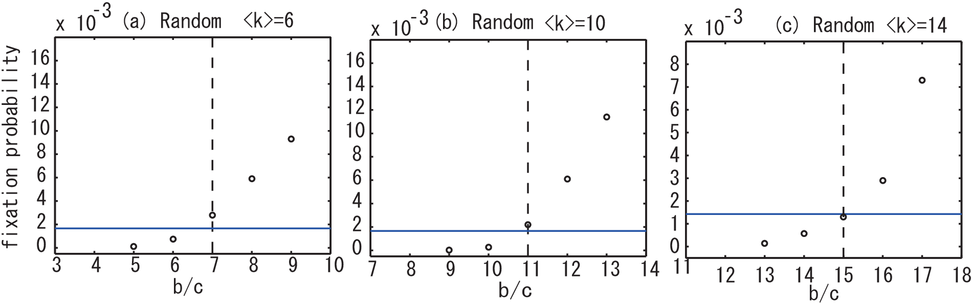

In the following, we show numerically that the condition (46) holds well, verifying our approximations. We simulate the game on several networks with set to different values. The random networks are Erdos-Reyni random networks [34]. The scale-free networks are made by a preferential attachment mechanism [35, 36]. In Fig. 6 and Fig. 7, the axis indicates , while the axis does the fixation probability. The horizontal straight line corresponds to the neutral probability given by . If a point is above the horizontal line, the network favors cooperation by definition; if the point is below the horizontal line, the network suppresses cooperation. The vertical broken line indicates the point where . Our condition holds exactly if a point falls onto the crossing of the horizontal and vertical lines. Figure 6 and Fig. 7 show that for both random and scale-free networks, our condition holds well.
We constructed the scale-free networks in the following way. First, we prepare a complete network consisting of vertices, in which all the vertices are connected to each other. Next, a new vertex with links enters into the existing network. The probability that the new vertex is connected to an existing vertex is where is the degree of vertex . Next, another new vertex enters the exiting network in the same way. After repeating this process, we have a scale-free network. As gets large enough the exponent of the degree distribution of the scale-free network asymptotically converges to . In the simulation, we use , , , and is such that , so that the exponent is .

In Fig. 8, we compare the random and the scale-free networks. The network size , , and the mean degree are taken to be the same. The comparison shows that random networks favor cooperation more than scale-free networks do, because the fixation probabilities for random networks are greater for all the points.
11 Conclusion
We study the Prisoner’s Dilemma game where the payoff matrix is given by
| (54) |
and analytically derive the condition of favoring cooperation for uncorrelated networks. The game is done under a death-birth process with weak selection. In summary, we obtained the following four results.
(i) Although it has been widely thought that is the condition of favoring cooperation, we show that is the condition. The mean degree of players competing for a vacant vertex is and the fitness of these adjacent players are determined by ; then, determines the outcome.
(ii) We show that among three representative networks, regular, random, and scale-free, a regular network favors cooperation the most and a scale-free network the least. This is because the condition depends on the mean degree of nearest neighbors, . Whereas the scale-free network has the largest mean degree of nearest neighbors, the regular network has the least for the same value of the mean degree .
(iii) In an ideal typical scale-free network characterized by the infinite number of vertices with , cooperation is unfeasible.
(iv) Although the scale-free network and the heterogeneous network favor cooperation in some cases, they suppress cooperation in our case. The scale-free network does not always favor cooperation irrespective of the game structure, although some occasionally believe so. Whether the scale-free network enhances or diminishes cooperation depends on details of the game.
(v) We show that if the number of players is small, then the cooperation is favored in scale-free networks.
This would not be the case if the condition were determined by the mean degree , since the mean degree is a fixed value determined by the exponent when the network size is large enough.
Acknowledgement
The author would like to thank Z.R. Struzik, N. Hatano, H. Ohtsuki, H. Yoshikawa, M. Kandori, M. Nakamaru, and two anonymous referees for their valuable comments, and Japan Society for the Promotion of Science for the financial support.
Appendix A The derivation of
In the present appendix, we derive in Eq. (27). First, we are going to study the case where increases. Suppose that a -player with degree that is linked to -players and -players in the neighborhood is randomly chosen. The probability that an -player is chosen is given by
| (55) |
where . The probability that the chosen -player changes the strategy from to is
| (56) |
If the -player changes the strategy from to , the conditional probability increases by
| (57) |
where we have used the fact that changes only of order , which will be confirmed later.
Note the factor in the numerator of Eq. (57). We are going to explain the reason of the factor in Fig. 9.

The conditional probability increases when a -player on the vertex 1 changes the strategy from to and the player is linked to an -player on the vertex 2. The point is that when both of the degrees of the vertex 1 and the vertex 2 are , the factor appears. Let A1 denote the strategy of the vertex 1 and A2 that of the vertex 2. Thus, both of the pairs A1–A2 and A2–A1 resulting from the change of strategy contribute to the increase in the conditional probability; one is seen from the vertex 1 and the other is seen from the vertex 2. When the vertex 1 was a -player, on the other hand, the pair was B1–A1. In the case of , from the assumption that a randomly chosen vertex has the degree and the vertices adjacent to the randomly chosen one has the degree the conditional probability would increase in one way seen from the vertex with the degree in Eq. (25).
Suppose that the vertex 1 changes the strategy from to ; then the pairs of and increases by one. On the other hand, suppose that the vertex 3 changes the strategy from to ; then the pairs of and increases by two. One is seen from the vertex 3 to 4 and the other is seen from the vertex 4 to 3.
Next, we are going to study the case where decreases. Suppose that an -player with degree linked to -players and -players in the neighborhood is randomly chosen to update the strategy. The probability that it happens is given by
| (58) |
The probability that the randomly chosen -player changes strategy from to is
| (59) |
If the -player changes the strategy from to B, then the conditional probability increases by
| (60) |
We thus have Eq. (27):
| (61) |
Appendix B The reason holds
In the present appendix, we argue the relation (31). The point is that in the mean-field approximation the degree of any randomly chosen vertex is , that of any neighboring degree is , and that of a vertex attached to a randomly chosen link is also . Note also that is the conditional probability between randomly chosen vertex and its neighbor, and is the conditional probability between vertices on both ends of a randomly chosen link.
Pair probabilities are computed by two methods. In one method, we first choose a vertex randomly and check the strategy of the vertex. Then, we check the strategies of all vertices linked to the chosen vertex. The conditional probability of finding a strategy on another vertex is . This procedure is carried out iteratively for all vertices. Because every link is connected to two vertices and every pair is counted twice, in this method, we count pairs in total, where denotes the number of links in the network. The pair probabilities computed by this method let us understand the relation .
In the other method of computing pair probability, we first choose a link and check the strategies of vertices of both ends of the chosen link. The probability of finding a strategy on one end is , and the conditional probability of finding a strategy on the other end given that the strategy is already found is . Then, we carry out this procedure iteratively for all links. In this method, we count pairs in total. The pair probabilities computed by this method let us understand the relation . Because of the mean-field relation , the term in Eq. (28) vanishes.
We also give another explanation of the relation . The pair probability is given by
| (62) |
and the pair probability is given by
| (63) |
Further, the relation holds. Therefore, the following equation holds:
| (64) | ||||
| (65) |
Because of the mean-field approximation we replace the degree of nearest neighbors by and the degree by :
| (66) | ||||
| (67) |
Therefore, holds in the mean-field approximation. Similarly, holds. Thus, holds in the mean-field approximation.
References
- [1] H. Ohtsuki, C. Hauert, E. Lieberman, M. A. Nowak, A simple rule for the evolution of cooperation on graphs and social networks, Nature 441 (7092) (2006) 502–505.
- [2] M. Nowak, Five rules for the evolution of cooperation, Science 314 (5805) (2006) 1560–1563.
- [3] M. A. Nowak, R. M. May, Evolutionary games and spatial chaos, Nature 359 (1992) 826–829.
- [4] J. Hofbauer, K. Sigmund, Evolutionary Dynamics and Population Dynamics, Cambridge University Press, 1998.
- [5] M. A. Nowak, A. Sasaki, C. Taylor, D. Fudenberg, Emergence of cooperation and evolutionary stability in finite populations, Nature 428 (2004) 646–650.
- [6] T. Killingback, M. Doebeli, Spatial evolutionary game theory: Hawks and doves revisited, Proc. R. Soc. Lond. B 263 (1996) 1135–1144.
- [7] M. Nakamaru, H. Matsuda, Y. Iwasa, The evolution of cooperation in a lattice-structured population, J. Theor. Biol. 184 (1997) 65–81.
- [8] M. van Baalen, D. A. Rand, The unit of selection in viscous populations and the evolution of altruism, J. Theor. Biol. 193 (1998) 631–648.
- [9] P. D. Taylor, T. Day, G. Wild, Evolution of cooperation in a finite homogeneous graph, Nature 447 (7143) (2007) 469–472.
- [10] J. Mitteldorf, D. S. Wilson, Population viscosity and the evolution of altruism, J. Theor. Biol. 204 (2000) 481–496.
- [11] M. Ifti, T. Killingback, M. Doebeli, Effects of neighbourhood size and connectivity on the spatial continuous prisoner’s dilemma, J. Theor. Biol. 231 (2004) 97–106.
- [12] E. Lieberman, C. Hauert, M. A. Nowak, Evolutionary dynamics on graphs, Nature 433 (2005) 312–316.
- [13] G. Szabo, J. Vukov, Cooperation for volunteering and partially random partnership, Phys. Rev. E 69 (2004) 036107.
- [14] D. S. Wilson, G. B. Pollock, L. A. Dugatkin, Can altruism evolve in a purely viscous population?, Evol. Ecol. 6 (1992) 331–341.
- [15] N. Masuda, Participation costs dismiss the advantage of heterogeneous networks in evolution of cooperation, Proceedings of the Royal Society B: Biological Sciences 274 (1620) (2007) 1815–1821.
- [16] S. Morita, Extended Pair Approximation of Evolutionary Game on Complex Networks, Progress of Theoretical Physics 119 (2008) 29–38.
- [17] C. Hauert, M. Doebeli, Spatial structure often inhibits the evolution of cooperation in the snowdrift game, Nature 428 (2004) 643–646.
- [18] S. N. Dorogovtsev, A. V. Goltsev, J. F. F. Mendes, Critical phenomena in complex networks, Reviews of Modern Physics 80 (4) (2008) 1275.
- [19] M. E. J. Newman, The structure and function of complex networks, SIAM Review 45 (2) (2003) 167–256.
- [20] G. Szabo, G. Fath, Evolutionary games on graphs, Physics Reports 446 (4-6) (2007) 97–216.
- [21] F. C. Santos, J. M. Pacheco, Scale-free networks provide a unifying framework for the emergence of cooperation, Phys. Rev. Lett. 95 (2005) 098104.
- [22] F. Santos, M. Santos, J. Pacheco, Social diversity promotes the emergence of cooperation in public goods games, Nature 454 (7201) (2008) 213–216.
- [23] F. Santos, J. Pacheco, T. Lenaerts, Evolutionary dynamics of social dilemmas in structured heterogeneous populations, Proceedings of the National Academy of Sciences 103 (9) (2006) 3490.
- [24] F. Fu, L. Wang, M. Nowak, C. Hauert, Evolutionary dynamics on graphs: Efficient method for weak selection, Physical Review E 79 (4) (2009) 46707.
- [25] R. Cohen, K. Erez, D. ben Avraham, S. Havlin, Resilience of the internet to random breakdowns, Phys. Rev. Lett. 85 (21) (2000) 4626–4628.
- [26] R. Pastor-Satorras, A. Vespignani, Epidemic spreading in scale-free networks, Physical Review Letters 86 (14) (2001) 3200.
- [27] R. Albert, H. Jeong, A. Barabasi, Attack and error tolerance of complex networks, Nature 406 (6794) (2000) 378–382.
- [28] J. Smith, G. Price, The logic of animal conflict, Nature 246 (5427) (1973) 15–18.
- [29] H. Ohtsuki, M. Nowak, The replicator equation on graphs, Journal of theoretical biology 243 (1) (2006) 86–97.
- [30] M. Nowak, Evolutionary Dynamics, Belknap Press, 2006.
- [31] H. Matsuda, N. Ogita, A. Sasaki, K. Sato, Statistical mechanics of population, Prog. Theor. Phys 88 (6) (1992) 1035–1049.
- [32] M. Kimura, J. Crow, An Introduction to Population Genetics Theory, Harper & Row, 1970.
- [33] N. van Kampen, Stochastic processes in physics and chemistry, North Holland, 1992.
- [34] P.Erdos, A.Renyi, On random graphs, Publicationes Mathematicae 6 (1959) 290–297.
- [35] A.-L. Barabasi, R. Albert, Emergence of scaling in random networks, Science 286 (5439) (1999) 509–512.
- [36] S. Dorogovtsev, J. Mendes, A. Samukhin, Structure of growing networks with preferential linking, Physical Review Letters 85 (21) (2000) 4633–4636.