Chiral magnetic effect in the PNJL model

We analyze, within the PNJL model, the response of quark matter to $\bm{B}$ at $\mu_{5}=0$. In particular we are interested in the interplay between chiral symmetry restoration and deconfinement crossover in the presence of a magnetic field which leads to the so-called chiral magnetic catalysis [14]. Our model parameter set is

These parameters correspond to $f_{\pi}=92.4\;\text{MeV}$ and the vacuum chiral condensate $\langle\bar{u}u\rangle^{1/3}=-245.7\;\text{MeV}$, and the constituent quark mass $M=339\;\text{MeV}$. The critical temperature for chiral restoration in the NJL part at $\bm{B}=0$ is $T_{c}\approx 190\;\text{MeV}$. We set the deconfinement scale $T_{0}$ in the Polyakov loop potential (see Eq. (6)) as $T_{0}=270\;\text{MeV}$, which is the value of the known deconfinement temperature in the pure $SU(3)$ gauge theory.

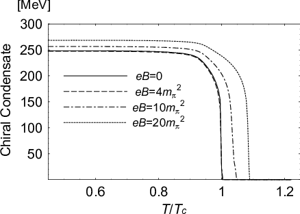
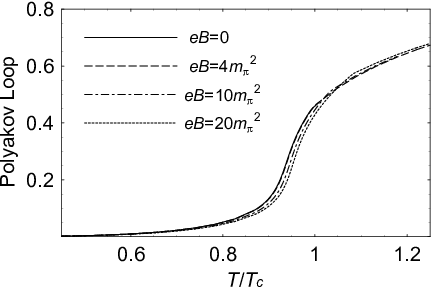
In Fig. 1 we plot the absolute value of the chiral condensate $\langle\bar{u}u\rangle^{1/3}$ (upper panel) and expectation value of the Polyakov loop (lower panel) as a function of $T$ computed at several values of $eB$ (expressed in unit of $m_{\pi}^{2}$). The chiral condensate $\langle\bar{u}u\rangle$ and the Polyakov loop $\Phi$ are the solution of the gap equations $\partial\Omega/\partial\sigma=\partial\Omega/\partial\Phi=0$ in the model at hand.

Figure 1 is interesting for several reasons. First of all, the role of $\bm{B}$ as a catalyzer of chiral symmetry breaking is evident. Indeed, the chiral condensate and thus constituent quark mass increase in the whole $T$ region as $eB$ is raised (for graphical reasons, we have plotted our results starting from $T=100\;\text{MeV}$. There is nevertheless no significant numerical difference between the $T=0$ and $T=100\;\text{MeV}$ results). This behavior is in the correct direction consistent with the well-known magnetic catalysis revealed in Ref. [14] and also discussed recently in Ref. [41] in a slightly different context of the PNJL-model study on the response of quark matter to external chromomagnetic fields.

Secondly, we observe that the deconfinement crossover is only marginally affected by the magnetic field. We can identify the deconfinement $T_{c}$ by the inflection point of $\Phi$ as a function of $T$. This simple procedure gives results nearly in agreement with those obtained by the peak position in the Polyakov loop susceptibility, which is a common prescription to locate the so-called pseudo-critical temperature. Also we can identify the deconfinement $T_{c}$ with the temperature at which $\Phi=0.5$. We note that $T_{c}$ in Fig. 1 is the chiral $T_{c}=228\;\text{MeV}$ where the chiral condensate vanishes, but not the deconfinement $T_{c}$ in both figures.

From Fig. 1 we notice that, increasing $eB$ from $4m_{\pi}^{2}$ to $20m_{\pi}^{2}$, the shift of the chiral transition temperature $\Delta T_{\chi}\approx 20\;\text{MeV}$, while the shift of the deconfinement crossover temperature is as small as $\Delta T_{\Phi}\approx 5\;\text{MeV}$. Hence, the chiral phase transition is more easily influenced by the magnetic field than the deconfinement as anticipated. Consequently, under a strong magnetic field, there opens a substantially wide $T$-window in which quarks are deconfined but chiral symmetry is still spontaneously broken. This result, valid for $\mu_{5}=0$, does not necessarily hold, in general, for $\mu_{5}\neq 0$, as we will see in the next subsection.

We next turn to the study of the effect of a finite $\mu_{5}$ on the QCD phase transitions using the PNJL model. We recall that $\mu_{5}$ cannot be a true chemical potential since its conjugate variable $n_{5}$ is only approximately conserved due to axial anomaly. Nevertheless, because the time derivative of the strong $\theta$ angle translates into $\mu_{5}$, as explained in the introduction section, $\mu_{5}$ itself is a physically meaningful quantity. We specifically look into the behavior of the critical line for chiral symmetry restoration, which is well defined in the chiral limit, at differing $\bm{B}$ while keeping $\mu_{5}$ fixed. This study will be useful, among other things, in order to understand the relation between the chirality density $n_{5}$ and $\mu_{5}$ that we compute numerically in later discussions.

One effect of $\mu_{5}\neq 0$ is lowering of the critical temperature of the chiral phase transition. This is evident from the upper panels of Fig. 2. Firstly we discuss the case of $eB=5m_{\pi}^{2}$ corresponding to the left upper and left lower panels of Fig. 2. We see that increasing $\mu_{5}$ at low $T$ results in slight enhancement of the chiral condensate. As $T$ approaches $T_{c}$, however, the chiral phase transition at larger $\mu_{5}$ takes earlier place below $T_{c}$. As a result of the coupling between the chiral condensate and the Polyakov loop, the deconfinement crossover as shown in the lower panels of Fig. 2 is also shifted earlier as $\mu_{5}$ becomes greater.

In view of the right upper and right lower panels of Fig. 2 for large $eB=10m_{\pi}^{2}$ the $\mu_{5}$-effect on the chiral condensate at low $T$ is less visible. This is understood from the fact that the chiral magnetic catalysis effect is predominant over the minor enhancement due to $\mu_{5}$. In contrast, as $T$ is increased toward $T_{c}$, the qualitative behavior of the shift in the critical temperature is just the same as what we have seen previously for $eB=5m_{\pi}^{2}$.

An interesting prediction from the PNJL model is that, at a given value of $eB$, there exists a critical $\mu_{5}$, above which the chiral phase transition becomes first order. In the case $eB=5m_{\pi}^{2}$ as shown in Fig. 2 the critical $\mu_{5}$ is found between $300\sim 400\;\text{MeV}$. As a matter of fact, at $\mu_{5}=400\;\text{MeV}$, the chiral condensate and the Polyakov loop both exhibit discontinuity at the critical temperature. We see that, as compared to the $\mu_{5}=300\;\text{MeV}$ case, the slopes of the chiral condensate and the Polyakov loop sharply change as a function of $T$ for the $\mu_{5}=400\;\text{MeV}$ case. Hence, our data plotted in Fig. 2 suggest the existence of a critical $\mu_{5}$ in the range $300\;\text{MeV}<\mu_{5}^{c}<400\;\text{MeV}$ at which the weakly first-order transition becomes a true second-order one. The phase diagram in the $\mu_{5}$-$T$ plane has a tricritical point (TCP) accordingly. We will discuss more on the TCP in the next subsection. We notice that this picture is qualitatively robust regardless of the chosen value of $eB$, as is already implied from Fig. 2. The first-order phase transition in the high-$mu_{5}$ and low $T$ region leads to a discontinuity in the chirality density as a function of $\mu_{5}$. This point will be also addressed in some details in the next section.

As a final remark in this subsection we note that, in Figs. 1 and 2, the slope of the curve quickly changes at some point (at $T/T_{c}=1$ for $eB=0$ for example). This is because of the second-order phase transition which is the case for chiral restoration in the chiral limit.

The results we have revealed so far can be summarized into the phase diagram in the $\mu_{5}$-$T$ plane. In the upper panel of Fig. 3 we show the phase diagram at $eB=5m_{\pi}^{2}$. In the lower panel for comparison we plot the phase diagram at $eB=15m_{\pi}^{2}$. The line represents the chiral phase transition. It is of second order for small values of $\mu_{5}$ (shown by a thin line) and becomes of first order at large $\mu_{5}$ (shown by a thick line). The location of the TCP on the phase diagram depends only slightly on $eB$, while the topology of the phase diagram is not sensitive to the magnetic field.

The general effect of $\mu_{5}$ is to lower the chiral transition temperature. One may argue that the critical line can hit $T=0$ eventually at very large $\mu_{5}$, though the PNJL model is of no use at such large $\mu_{5}$ because the ultraviolet cutoff causes unphysical artifacts. The locations of the TCP are estimated from the PNJL model as

The axial anomaly relates the topological charge $Q_{W}$ to the chirality charge $N_{5}$ with $N_{5}=n_{5}V$ where $V=L_{x}L_{y}L_{z}$ is the volume of topological domains. We can read $n_{5}$ from

It is useful information to relate $n_{5}$ and $\mu_{5}$ for various temperatures and magnetic field strength. In the next section we will use the results of $n_{5}(\mu_{5})$ to express the current density as a function of the chirality density.

The relation between $n_{5}$ and $\mu_{5}$ can be found analytically only in simple limiting cases [19]. In general one has to determine it numerically using an effective model. We show $n_{5}(\mu_{5})$ for $eB=5m_{\pi}^{2}$ at three temperatures around $T_{c}$ in Fig. 4. The qualitative picture is hardly modified even if we change the magnetic field.

From Fig. 3 we can read the critical temperature at $\mu_{5}=0$ that is $T_{c}=228\;\text{MeV}$. At temperatures well below $T_{c}$, as seen in the $T=160\;\text{MeV}$ case in Fig. 4, the discontinuity associated with the first-order phase transition with respect to $\langle\bar{u}u\rangle^{1/3}$ and $\Phi$ is conveyed to the relation $n_{5}(\mu_{5})$, which is a typical manifestation of the mixed phase at critical $\mu_{5}$. Naturally, as $T$ gets larger, the chirality density as a function of $\mu_{5}$ becomes smoother, since the chiral phase transition is of second order at higher $T$ as is clear from Fig. 3.

It is interesting to compute the chirality charge susceptibility $\chi_{5}$, as well as $n_{5}$, defined as

where $\beta=1/T$ and $V$ the volume. We note that this definition of the susceptibility is different from that in Ref. [27] by $V$. It should be mentioned that we take a numerical derivative to compute $\chi_{5}$ including implicit dependence in $\Phi$ and $\sigma$. In Fig. 5 we plot $\chi_{5}$ as a function of $eB$ for several $\mu_{5}$ values. The upper panel corresponds to $\mu_{5}=0$, middle one to $\mu_{5}=200\;\text{MeV}$, and lower one to $\mu_{5}=400\;\text{MeV}$. For completeness, in the right panels of the same figure 5 we plot the chiral condensate $|\langle\bar{u}u\rangle^{1/3}|$ for the same $T$ and same $\mu_{5}$. The oscillations in $\chi_{5}$ are artificial results because of the momentum cutoff $\Lambda$. As shown in Ref. [41], choosing a regulator which is smoother than used in this work, the oscillations of the various quantities could be erased. The qualitative picture is, nevertheless, unchanged even with a different regulator. For this reason we do not perform a systematic study here on the cutoff scheme dependence.

A notable aspect is the suppression of the chirality-charge fluctuations at large $T$ and large $eB$. This is evident, for example, in the result with $\mu_{5}=0$ and $T=1.1T_{c}$ in Fig. 5. As long as $eB$ is small, $\chi_{5}$ is a monotonously increasing function of $eB$ as expected naively. When $eB$ reaches a critical value around $20m_{\pi}^{2}$, however, $\chi_{5}$ has a pronounced peak and then decreases with increasing $eB$, which is a result of mixture with diverging chiral susceptibility at the chiral phase transition. It should be mentioned that $\chi_{5}$ at $\mu_{5}=0$ (as shown in the upper left panel of Fig. 5) does not diverge at the critical $eB$ since the mixing with the chiral susceptibility is vanishing due to $\mu_{5}=0$. This behavior below and above the chiral critical point can be easily understood in terms of the chiral symmetry breaking by virtue of the magnetic field. As a matter of fact, at $T>T_{c}$ the chiral condensate stays zero identically as long as $eB$ is small enough, leading to zero quasiparticle masses. Once $eB$ exceeds a critical value, the chiral symmetry is broken spontaneously even at high $T$ (see the upper right panel of Fig. 5) and the quasiparticle masses can then jump to a substantially large number then. Such dynamical quark masses result in appreciable suppression of the chirality-charge fluctuations. As it will be shown in the next section, this interesting and intuitively understandable effect appears in the current susceptibility as well.

The current density $j_{3}$ (and its susceptibility as well) is the most important quantity to compute for the Chiral Magnetic Effect [27]. It corresponds to the charge per unit volume that moves in the direction of the applied magnetic field in a domain where an instanton/sphaleron transition takes place, which causes chirality change of quarks. The current has been computed analytically in Ref. [19] in four different ways.

To compute the current density along the magnetic field, i.e. $j_{3}=q\langle\bar{\psi}\gamma_{3}\psi\rangle$, we follow the common procedure to add an external homogeneous vector potential along the magnetic field, $A_{3}$, coupled to the fermion field. Then,

The derivative of the thermodynamic potential in the presence of a background field is computed in the following way. The coupling of quarks to $A_{3}$ is achieved by shifting $p_{z}$ in Eq. (10) as $p_{z}\rightarrow p_{z}+q_{f}A_{3}$. After putting regularization in the momentum integral with an ultraviolet cutoff $\Lambda$ (we know that the current is ultraviolet finite, hence the choice of the regularization method does not affect the final result) we change the order of the momentum integral and the derivative with respect to $A_{3}$. Then we make use of the following replacement,

to obtain,

The ellipsis represents irrelevant matter terms. After summing over the spin $s$, the contribution of the integrand from the Landau levels with $n>0$ turns out to be an odd function of $p_{z}$. Therefore, only the lowest Landau level gives a non-vanishing contribution to the current and we get from the surface contribution [19],

which is certainly ultraviolet finite as it should be. Generally speaking we should utilize a gauge-invariant regularization. Nevertheless the above (21) indicates that a naive momentum cutoff can reproduce a correct expression for the anomalous chiral magnetic current.

The current density as given by Eq. (21) does not depend on quark mass explicitly, and on temperature either. The reason is that the current is generated by the axial anomaly and it receives contributions only from the ultraviolet momentum regions (as the above derivation shows), and so it is insensitive to any infrared energy scales. Also, the Polyakov loop does not appear explicitly in Eq. (21). This is easy to understand; the Polyakov loop is a thermal coupling between quark excitations and the gluonic medium, and thus the Polyakov loop only enters the thermal part of $\Omega$. Since the current originates from the anomaly, however, the thermal part of $\Omega$ just drops off for the current generation. The effect of the Polyakov loop will appear implicitly through the relation between $\mu_{5}$ to $n_{5}$.

To confirm that our numerical prescription works well, we have computed $j_{3}$ by means of Eq. (18) with $\Omega$ given in Eq. (10). In Fig. 6 we show the results from our numerical computation as a function of $\mu_{5}$. In the figure we have plotted the normalized current,

with a choice of $\mu_{0}=1\;\text{GeV}$, which we defined so to make the comparison transparent at a glance. In Fig. 6 the dashed line represents $\tilde{j}_{3}$ at $T=160\;\text{MeV}$; on the other hand, the dot-dashed line the case at $T=240\;\text{MeV}$. We notice that our numerical results are perfectly in agreement with Eq. (21). We conclude that our numerical procedure correctly reproduces the expected dependence of $j_{3}$ on $\mu_{5}$ with the correct coefficient insensitive to infrared scales regardless of whether $T$ is below or above $T_{c}$.

The result shown in the upper panel of Fig. 6 gives us confidence in our numerical procedure but the figure itself is not yet more informative than Eq. (21). We express now $j_{3}$ as a function of $n_{5}$ using Eq. (21) and the results discussed in the previous section. The result of this computation is shown in the lower panel of Fig. 6, in which we plot the (not normalized) current density (measured in fm^-3) as a function of $n_{5}$ (measured in fm^-3), at $eB=5m_{\pi}^{2}$ and at three different temperatures.

From Fig. 6 we notice that, at a fixed value of $n_{5}$, the larger the temperature is, the smaller $j_{3}$ becomes. This seemingly counter intuitive result is easy to understand. As a matter of fact, as the temperature gets larger, the corresponding $\mu_{5}$ for a given $n_{5}$ should decrease because of more abundant thermal particles at higher temperature. Since $j_{3}$ depends solely on $\mu_{5}$, a higher temperature requires a larger $n_{5}$ to give the same $j_{3}$.

Besides $j_{3}$, another interesting quantity is the current susceptibility defined by

If we naively use the above definition (23) for the cutoff model like the PNJL model, $\chi_{J}$ is non-zero proportional to $\Lambda^{2}$ even at $T=B=0$ as discussed in Ref. [27]. This is in contradiction with the gauge invariance, which requires the above susceptibility to vanish because the current susceptibility is nothing but the $33$-component of the photon polarization tensor at zero momentum. Therefore, in order to deal with the physically meaningful quantity, we subtract the vacuum part from the above equation and compute,

to fulfill the requirement that photons are unscreened at $T=B=0$ regardless of any value of $\mu_{5}$.

We plot our results for $\beta V\bar{\chi}_{J}$ as a function of $eB$ in Fig. 7 at $\mu_{5}=0$ (upper panel), $\mu_{5}=200\;\text{MeV}$ (middle panel), and $\mu_{5}=400\;\text{MeV}$ (lower panel). The oscillations in the susceptibility behavior are an artifact of the momentum cutoff. In these plots $T_{c}=228\;\text{MeV}$ denotes the critical temperature for chiral symmetry restoration at $\mu_{5}=B=0$.

Let us first focus on the case at $\mu_{5}=0$. At $T=0$ and $T=0.95T_{c}$ the system is in the broken phase with $\langle\bar{u}u\rangle\neq 0$ over the whole range of $eB$. On the other hand, at the temperature $T=1.1T_{c}$, the system is in the chiral symmetric phase for $eB$ smaller than a critical value. There is a phase transition from the symmetric to the broken phase with increasing $eB$. This transition is driven by the presence of the magnetic field as the catalysis of chiral symmetry breaking, as mentioned before. The effect of the phase transition leads to a cusp in the susceptibility $\chi_{J}$ as a function of $eB$. We also notice that there seems to exist a range in $eB$ in which $\bar{\chi}_{J}<0$. This is a mere artifact of the momentum cutoff, which causes unphysical fluctuations in $\bar{\chi}_{J}$. The qualitative picture is similar also at $\mu_{5}\neq 0$.

To distinguish physically meaningful information from cutoff artifacts, we have computed $\chi_{J}$ using a smoother regulator with $N=5$ in Eq. (12). We have readjusted the NJL parameters to keep the physical quantities ($f_{\pi}$ and $\langle\bar{u}u\rangle$) unchanged. Figure 8 is the result in which oscillations are suppressed and $\chi_{J}>0$ for any $T$ and $B$.

In view of Figs. 7 and 8 we can conclude that it is certainly a physical effect that the chiral phase transition critically affects the susceptibility $\chi_{J}$ as well as $\chi_{5}$. As shown in Ref. [27] the susceptibility difference between the longitudinal and transverse directions has an origin in the axial anomaly and is insensitive to the infrared information. Nevertheless, $\chi_{J}$ (and transverse $\chi_{J}^{T}$ too) should be largely enhanced near the chiral phase transition through mixing with the divergent chiral susceptibility, which is not constrained by anomaly. Such enhancement in $\chi_{J}$ would ease the confirmation of the CME signals at experiment.