The universal distribution of halo interlopers
in projected phase space
Abstract
When clusters of galaxies are viewed in projection, one cannot avoid picking up a fraction of foreground/background interlopers, that lie within the virial cone, but outside the virial sphere. Structural and kinematic deprojection equations are known for the academic case of a static Universe, but not for the real case of an expanding Universe, where the Hubble flow (HF) stretches the line-of-sight distribution of velocities. Using 93 mock relaxed clusters, built from the dark matter (DM) particles of a hydrodynamical cosmological simulation, we quantify the distribution of interlopers in projected phase space (PPS), as well as the biases in the radial and kinematical structure of clusters produced by the HF. The stacked mock clusters are well fit by an =5 Einasto DM density profile (but only out to 1.5 virial radii), with velocity anisotropy (VA) close to the Mamon-Łokas model with characteristic radius equal to that of density slope . The surface density of interlopers is nearly flat out to the virial radius, while their velocity distribution shows a dominant gaussian cluster-outskirts component and a flat field component. This distribution of interlopers in PPS is nearly universal, showing only small trends with cluster mass, and is quantified. A local =2.7 sigma velocity cut is found to return the line-of-sight velocity dispersion profile (LOSVDP) expected from the NFW density and VA profiles measured in three dimensions. The HF causes a shallower outer LOSVDP that cannot be well matched by the Einasto model for any value of . After this velocity cut, which removes 1 interloper out of 6, interlopers still account for 23% of all DM particles with projected radii within the virial radius (surprisingly very similar to the observed fraction of cluster galaxies lying off the Red Sequence) and over 60% between 0.8 and 1 virial radius. The HF causes the best-fit projected NFW or =5 Einasto model to the stacked cluster to underestimate the true concentration measured in 3D by 66% (167%) after (before) the velocity cut. These biases in concentration are reduced by over a factor two once a constant background is included in the fit. The VA profile recovered from the measured LOSVDP by assuming the correct mass profile recovers fairly well the VA measured in 3D, with a slight, marginally significant, bias towards more radial orbits in the outer regions. These small biases in the concentration and VA of the galaxy system are overshadowed by important cluster-to-cluster fluctuations caused by cosmic variance and by the strong inefficiency caused by the limited numbers of observed galaxies in clusters. An appendix provides an analytical approximation to the surface density, projected mass and tangential shear profiles of the Einasto model. Another derives the expressions for the surface density and mass profiles of the NFW model projected on the sphere (for future kinematic modeling).
Key Words.
Galaxies: clusters: general — Cosmology: miscellaneous — (Cosmology): dark matter — Galaxies: halos — Gravitational lensing: weak — Methods: numerical1 Introduction
The galaxy number density profiles of groups and clusters of galaxies falls off slowly enough at large radii that material beyond the virial radius (within which these structures are thought to be in dynamical equilibrium) contribute non-negligibly to the projected view of cluster, i.e. to the radial profiles of surface density, line-of-sight velocity dispersion and higher velocity moments.
In principle, this contamination of observables by interlopers, defined here as particles that lie within the virial cone but outside the virial sphere, is not a problem, since we know how to express deprojection equations when interlopers extend to infinity along the line-of-sight. Consider the projection equation
| (1) |
where and are the projected and space number densities, respectively, while and are the projected and space radial distances (hereafter, radii), respectively. Equation (1) can be deprojected through Abel inversion11 1 Alternatively, the projection equation (1) corresponds to a convolution and can therefore be deprojected with Fourier methods (see Discussion in Mamon & Boué 2010 and references therein). to yield
| (2) |
The projection to infinity is explicit in equations (1) and (2).
However, the Hubble expansion complicates the picture, as the Hubble flow moves background (foreground) objects to high positive (negative) line-of-sight velocities.


This is illustrated in Figure 1 which shows how the line-of-sight velocity vs. real-space distance relation is affected by the Hubble flow. The line-of-sight distances are computed as the segment length QP in Figure 2.

Now, clipping the velocity differences to, say, times the cluster velocity dispersion (averaged over a circular aperture, hereafter aperture velocity dispersion), , gets rid of all the distant interlopers. More precisely, the radius, , where the Hubble flow matches is found by solving (where is the Hubble constant) yielding
| (3) |
where is the virial radius where the mean density is times the critical density of the Universe, (where is the gravitational constant), and where is the circular velocity at the virial radius. Clusters are thought to have density profiles consistent with the Navarro, Frenk, & White profile (1996, hereafter NFW) profiles,
| (4) |
where is the radius of density slope , in number (Lin, Mohr, & Stanford 2004), luminosity (Łokas & Mamon 2003) and mass (Łokas & Mamon; Biviano & Girardi 2003; Katgert, Biviano, & Mazure 2004), with a concentration, , of 3 to 5. For isotropic NFW models, the aperture velocity dispersion is (Appendix A of Mauduit & Mamon 2007) , where (weakly dependent on concentration), and equation (3) then becomes
| (5) |
Equation (5) indicates that a 3-sigma clipping will remove all material beyond 13 () or 19 () virial radii.22 2 With our chosen cosmology, the overdensity at the virial radius is , but many authors prefer to work with , and we will do so too. So, in the deprojection equation (2), the upper integration limit must be set to this value of . Although this effective cutoff in line-of-sight distances is quite far removed from the cluster, it is not clear whether there may still be a measurable bias in the concentration of clusters that one measures by comparing the surface density distribution of galaxies in clusters with NFW models projected out to infinity. Moreover, it is not clear how accurate are such measures given the finite number of galaxies observed within clusters.
Finally, it is not clear how the stretching of the velocities affects the kinematic analyses of clusters, especially in the case of nearby clusters where the opening angle of the cone is non-negligible, leading to an asymmetry between the foreground and background absolute velocity distributions. For example, is the anisotropy of the 3D velocity distribution (hereafter velocity anisotropy or simply anisotropy)
| (6) |
or equivalently33 3 enters the Jeans equation of local hydrostatic equilibrium, while is a more physical definition of velocity anisotropy.
| (7) |
affected by the Hubble flow? One can add interlopers beyond the virial radius as a separate component to the kinematical modeling (van der Marel et al. 2000; Wojtak et al. 2007). Unfortunately, we have no knowledge of the distribution of interlopers in projected phase space (projected distance to the halo center and line-of-sight velocity).
This paper provides the distribution of interlopers in projected phase space (projected distance to the halo center and line-of-sight velocity) as measured on nearly 100 stacked halos from a well-resolved cosmological simulation. We additionally measure the bias in the measured surface density and line-of-sight velocity dispersion and kurtosis profiles compared to those obtained in a Universe with no Hubble flow, and estimate how this bias affects the recovered concentration and velocity anisotropy of the cluster. In this paper, we use interchangeably the terms ‘clusters’ and ‘halos’.
We present in Sect. 2 the cosmological simulations we use and how the individual halos were built. In Sect. 3 we explain how we stack these halos. In Sect. 4, we present the statistics on the halo members and the interlopers in projected phase space. Then in Sect. 5, we explain how we remove the outer interlopers and show analogous statistics on the cleaned stacked halo in Sect. 6. We proceed in Sect. 7 to measure the biases induced by the Hubble flow and the imperfect interloper removal on the estimated concentration parameter and anisotropy profile. We discuss our results in Sect. 8.
2 Data from cosmological -body simulations
The halos analyzed in this paper were extracted by Borgani et al. (2004) from their large cosmological hydrodynamical simulation performed using the parallel Tree+SPH GADGET–2 code (Springel 2005). The simulation assumes a cosmological model with present day parameters , , , , and . The box size is Mpc. The simulation used dark matter particles and (initially) as many gas particles, for a dark matter particle mass of . The softening length was set to until and fixed afterwards (i.e., kpc). The simulation code includes explicit energy and entropy conservation, radiative cooling, a uniform time-dependent UV background (Haardt & Madau 1996), the self-regulated hybrid multi-phase model for star formation (Springel & Hernquist 2003), and a phenomenological model for galactic winds powered by Type-II supernovae.
Dark matter halos were identified by Borgani et al. at redshift by applying a standard Friends-of-friends (FoF) analysis to the dark matter particle set, with linking length 0.15 times the mean inter-particle distance. After the FoF identification, the center of the halo was set to the position of its most bound particle. A spherical overdensity criterion was then applied to determine the virial radius, of each halo. In this manner, 117 halos were identified within the simulated volume, among which 105 form a complete subsample with virial mass larger than , thus representing a sample of mock galaxy clusters. Their mean and maximum masses are respectively and .
To save computing time, we worked on a random subsample of roughly 2 million particles among the . Although the simulation also produced galaxies, we chose to use the dark matter particles as tracers of the galaxy distribution for two reasons: 1) Simulated galaxy properties in cosmological simulations depend on details of the baryon physics implemented in the code, and can show some mismatch with observed properties (e.g. Saro et al. 2006); 2) only a handful of simulated clusters had over 50 galaxies (Saro et al.), so we would have strongly suffered from small-number statistics. There is some debate on whether the velocity distribution of galaxies is biased relative to the dark matter. On one hand, the galaxy velocity distribution, although close to the dark matter one, shows a preference for lower velocities (Biviano et al. 2006), perhaps as a consequence of dynamical friction. On the other hand, the velocity distribution of subhalos, selected with a minimum mass before entering their parent cluster-mass halos, is similar to that of the dark matter (Faltenbacher & Diemand 2006).
We visually inspected each of the 105 clusters in redshift space along three orthogonal viewing axes, and removed 12 clusters that appeared, within , to be composed of two or three sub-clusters of similar mass (where the secondary had at least 40% of the mass of the primary). Most observers would omit such clusters when analyzing their radial structure or internal kinematics. This leaves us with 93 final mock clusters.44 4 Including all 105 halos makes virtually no difference for the results of this article. The median values (interquartile uncertainties) of their virial radii, virial masses, virial circular velocities, and velocity dispersions (within their virial spheres) are respectively 864, 1.50, 865, and 584.
3 Stacking the virial cones
For each cluster, we projected the coordinates along the virial cone (circumscribing the virial sphere, see Fig. 2), as follows. We first renormalized the 6 coordinates of phase space of the entire simulation box to be relative to the cluster. So the cluster most bound particle should be at the origin and its mean peculiar (bulk) velocity should be zero.55 5 Observers usually adopt the position of the brightest cluster galaxy as the center, and this corresponds to the most bound galaxy, so they should not suffer from important centering errors, although admittedly some clusters like Coma have two brightest galaxies. To take into account the periodic boundaries of the simulation box, we added or subtracted a box length to those particles situated at over a half-box length from the cluster center. In this fashion, each cluster now effectively sits at the center of the simulation box. We then placed an observer at coordinates , , or , with . We present here the results for , corresponding to a typical distance of observed clusters in the local Universe. At this distance, the median virial angular radius of our 93 clusters is 33. We do not expect that the results of this paper should depend on the adopted value of . We assume that the observer’s peculiar velocity is equal to the cluster’s bulk velocity, so that the observer’s velocity is zero in the renormalized coordinate system.66 6 In our simulation, the one-dimensional cluster bulk velocity dispersion is , so given our adopted distance of , the typical cluster bulk velocity is only . Therefore, our neglect of the observer’s peculiar motion relative to the cluster is an adequate assumption.
We then measured, for each cluster and for each of these three observers, the coordinates of all 2 million particles in both the observer frame and the cluster frame. Given the distance of the particle to the observer and the projected coordinate of the particle in cylindrical coordinates , we determined the projected distances in the observer frame (measured in a plane perpendicular to the line-of-sight passing through the cluster center) as (see Fig 2, where , , , and ). This projection ensures that particles along the surface of the virial cone have . We were then able to select all particles within a cone circumscribing the sphere of radius , where we chose , as well as . In practice, we extracted data from a wider cone, circumscribing the sphere of radius .
We next added the Hubble flow (for both the observer and cluster frames), using .77 7 All our positions and cluster virial radii were expressed in ; the choice of does not matter as long as we normalize to the virial quantities and , which we computed with the same value of . We then limited in depth to line-of-sight velocities within from the cluster. As mentioned in Sect. 1, the Hubble flow effectively limits the depth of the cones to a half-length of virial radii (see eq. [3]), where the cut in velocity space in units of virial velocity is and the virial overdensity is .88 8 Throughout this paper, we use to express quantity in virial units. Our results should not depend much on the distance of our observer ( virial radii), as our first cut at 4 virial velocities limits the line of sight to 40% of the observer’s distance.
We finally normalized the particle relative positions and velocities to the virial radius, and circular velocity at the virial radius, , respectively, and finally computed the projections of the velocities in spherical coordinates (to later measure the 3D radial profiles of density and velocity anisotropy). For clarity, we will sometimes use the notation for the virial radius and for the virial velocity.
In the end, we have roughly 84 thousand particles for each of the three cartesian stacked virial cones, which we then stack together into our global stacked virial cone, with a grand total of roughly a quarter-million particles, among which nearly three-quarters lie within the virial radius. Hence, roughly 1/30th of all the particles in the simulation box lie within the virial radius, , of our 93 clusters. Note that with our stacking method, some of the particles inside virial cones but outside virial radii can end up being selected in more than one of the three cartesian stacked virial cones. However, this fraction is small (27% of the interlopers, i.e. less than 8% of all particles in virial cones), so the three cartesian stacked virial cones are virtually independent (except that their halos are common), hence can be stacked into the global virial cone.

Figure 3 shows the projected phase space (line-of-sight velocity, , versus projected radius, ) distribution of particles of the stacked cluster, highlighting the halo particles (lying within the virial sphere) and interlopers (lying in the virial cone but outside of the virial sphere). Note that the halo particles are confined to fairly small velocities (the largest absolute halo particle velocity is ). One notices an excess of positive velocity outliers in comparison with negative velocity ones, as expected from the conical projection used here.
4 Interloper statistics before the velocity cut
We now measure the distribution of interlopers in projected phase space and study its dependence on halo mass.
4.1 Global statistics

Figure 4 displays contours of the density in projected phase space. Note that the projected phase space density of Figure 4 is proportional to , hence the different shapes than seen in Figure 3. The interlopers have a very different projected phase space density than the halo particles. In particular, their horizontal contours mean that the interloper projected phase space density is fairly independent of projected radius. Moreover, the interloper contours do not extend beyond , except for a few islands (caused by cosmic variance), indicating that the velocity distribution of interlopers is close to flat at large velocities (the islands thus represent small, probably statistical, fluctuations in a flat background).
These issues can be looked in more detail through slices of the projected phase space density in velocity and radial space.
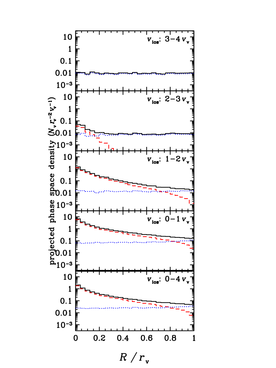
Figure 5 shows how the projected phase space density varies with projected radius in different wide velocity bins. The halo particles display a negative gradient, i.e. a decreasing surface number density profile, as expected. However, one immediately notices that in all line-of-sight velocity bins, the density of interlopers in projected phase space is roughly independent of projected radius. In other words, interlopers have a nearly flat surface density profile.
For low velocities, one can notice a small rise of the interloper surface density at high projected radii. This small rise is a geometric effect: the line-of-sight distance between the virial sphere and a sphere of virial radii is virial radii at but virial radii at , which is times greater. We will return to this rise in Sect 4.2.

Figure 6 displays the distribution of line-of-sight velocities of the halo and interloping particles. The interloper distribution shows a flat component that dominates at large velocities and a gaussian-like component. Figure 6 confirms, once more (see Figs. 4 and especially 5) that the density of interlopers in projected phase space is fairly independent of radius.
The total surface density of particles in velocity space shows an inflection point at about (bottom plot of Fig. 6). Kinematical modelers attempt to throw out the high-velocity interlopers by identifying this gap by eye (Kent & Gunn 1982; Łokas & Mamon 2003) or automatically (Fadda et al. 1996) or by rejecting outliers, either using a global criterion (Yahil & Vidal 1977) or a local one (e.g. Łokas et al. 2006; Wojtak & Łokas 2010). Interestingly, the criterion was first motivated on statistical grounds, but the inflection point one sees in the plots of Figure 6 happens to correspond to . In other words, the criterion is not only a consequence of statistics, but also motivated by the combination of cluster dynamics and cosmology.
While visual attempts to separate interlopers from halo particles in projected phase space look for gaps in the line-of-sight velocity distribution, the different panels of Figure 6 indicate that, on average, one should not expect such gaps in the projected phase space diagram of stacked clusters, as the number of interlopers also decreases with velocity to reach a plateau at about .
4.2 Universality

The three panels of Figure 7 illustrate the universality of the line-of-sight velocity distribution of interlopers, in terms of projected radius and halo mass. Figure 7a confirms that the projected phase space density of interlopers depends little on projected radius. This will be quantified later in this sub-section.
As mentioned above, to first order, the density of interlopers in projected phase space has a constant component and a quasi-gaussian component, which we write
| (8) |
Maximum likelihood estimation (MLE, see appendix C) yields
| (9) | |||||
where is in units of , while , and are in units of , where is the number of particles within the virial sphere. Figures 7a and 7c show that this gaussian+constant model is an excellent fit to the distribution of interloper line-of-sight velocities.
The origin of these two components is clarified in Figure 7b: cutting the halo interlopers in two subsamples at different 3D distances from the halo, one finds that the flat component corresponds roughly to the interlopers beyond , while the quasi-gaussian component corresponds to the closer interlopers ().
Figure 8 shows the radial dependence of the parameters of the interloper phase space distribution. We also show the mean surface densities of interlopers measured on the stacked halo.

The normalization of the gaussian component and the surface density both increase slowly at small projected radii, but sharply near the virial radius. A good fit for the normalization and the standard deviation of the gaussian component is provided by
| (10) | |||||
| (11) |
where and .
The solid magenta curve of Figure 8 indicates that the interloper surface density profile is well recovered from , and by integrating over the model velocity distribution (eq. [8]) from 0 to :
| (12) |
Alternatively, the surface density profile of interlopers is also well recovered (dashed magenta curve in Fig. 8) by the prediction from an NFW model, i.e. as the difference between the standard surface density integrated to infinity and the surface density limited to the virial sphere:
| (13) |
where the expression for is provided in equation (B.1). According to equation (13), the rise at radii close to the virial radius is almost independent of the concentration (with relative differences of less than 4% at all projected radii). Hence, one can adopt a unique empirical model for . These two estimates of are in very good agreement, except that the difference of the cylindrical and spherical NFW surface density profiles (eq. [13]) rises somewhat faster than our fit at projected radii very close to the virial radius.
The bottom panel of Figure 7 shows that the density of interlopers in projected phase space as a function of line-of-sight velocity remains the same for low and high mass clusters (where we took the dividing line at the median cluster virial mass of ). The interlopers of high mass clusters have a cluster-outskirts component whose density in projected phase space is roughly 15% lower than that of the low-mass clusters.

Figure 9 provides a closer look at the variation with halo mass of the parameters of equation (8). The best fitting logarithmic slopes, obtained by least-squares fits to the points shown in Fig. 9 are , , and for , , , and , respectively. The 90% confidence lower limits on the slopes are thus , , and for , , , and , respectively, while the 90% upper limits are less than 0.1 except for (where is it 0.5). These shallow limits to the logarithmic slopes illustrate the near-universality of the distribution of interlopers in projected phase space.
However, the universality of the distribution of interlopers in projected phase space may hide an important level of cosmic variance. Performing MLE for parameters , , and , for each of the 93 clusters, each viewed in turn along each of three orthogonal viewing axes, we find standard deviations of
| (14) |
So, while the dispersion of the gaussian component of the interloper velocity distribution is fairly constant (29% typical variations) from one cluster to the next, there is more scatter in the normalization of the gaussian component (factor 1.7 typical variations) and a large scatter in the flat component (factor 2.5 typical variations).
5 Interloper removal
We remove the interlopers of the stacked cluster proceeding along similar lines as Łokas et al. (2006) (see also Wojtak et al. 2007), by clipping the velocities beyond times the local line-of-sight velocity dispersion. We assume that our stacked cluster has an NFW profile (eq. [4]), or, alternatively, an Einasto (1965) profile:
| (15) |
where is the incomplete gamma function. The density model of equation (15) fits the density profiles of CDM halos even better than the NFW model (as first discovered by Navarro et al. 2004), at the expense of an additional parameter, .
The velocity cut requires an estimate of the line-of-sight velocity dispersion profile of the halo. One could measure this in bins of projected radius, iteratively rejecting the outliers. This gives a profile that shows important radial fluctuations, and we would need to either smooth the profile or fit a smooth analytical function to it.
Instead, we choose to predict the line-of-sight velocity dispersion profile given the typical density and velocity anisotropy profiles of halos. The line-of-sight velocity dispersion profile can be written (Mamon & Łokas 2005b)
| (16) |
where is the circular velocity profile, is the anisotropy radius, while the dimensionless kernel is
| (17) |
for isotropic orbits (Tremaine et al. 1994; Prugniel & Simien 1997) and
| (18) |
where
| (19) |
(Mamon & Łokas 2005b) for the anisotropy profile
| (20) |
which Mamon & Łokas (2005b) (hereafter, ML) found to be a good fit to the anisotropy profiles of CDM halos.
Since the space density model enters equation (16) expressing (through the tracer density and the total mass , which are related since we are considering single component mass models), we first need to determine the best fitting model to the distribution of particle radii in the stacked halo: we performed MLE of the NFW and Einasto models to the distribution of 3D radii of our stacked cluster. The minimum radius was chosen as to avoid smaller radii, since our halo centers appear to be uncertain to about 1% of the virial radius. We varied the outer radii of the fit, starting at . Since we will later fit the surface density profile out to the virial radius and beyond, we need to remember that the space radii extend beyond the maximum projected radius of the future surface density fits. So we also performed 3D fits beyond the virial radius: at (which corresponds to the radius where , i.e. the largest radius where the halos should be close to virial equilibrium), and for a broader view of halos far beyond .
When Prada et al. (2006) fit the density profiles of CDM halos out to , they found them to be well approximated by the sum of an Einasto model and a constant term . We therefore also experimented with the addition of a constant background component of density equal to the density of the Universe. In virial units, this background is expected to be equal to (with and ).
| Model | ||||
|---|---|---|---|---|
| NFW | 1 | 0 | 4.080.050.17 | 0.0021 |
| NFW | 1 | (0.036) | 4.100.050.17 | 0.0023 |
| NFW | 1 | 0.416 | 4.260.070.23 | 0.0069 |
| Einasto | 1 | 0 | 4.000.050.17 | 0.31 |
| Einasto | 1 | (0.036) | 4.020.050.17 | 0.3 |
| Einasto | 1 | 0.002 | 4.000.070.20 | 0.31 |
| NFW | 1.35 | 0 | 4.200.050.14 | 0.0023 |
| NFW | 1.35 | (0.036) | 4.230.050.14 | 0.0021 |
| NFW | 1.35 | 0.002 | 4.200.040.15 | 0.002 |
| Einasto | 1.35 | 0 | 4.140.040.13 | 0.016 |
| Einasto | 1.35 | (0.036) | 4.170.040.13 | 0.0058 |
| Einasto | 1.35 | 0.002 | 4.140.040.14 | 0.015 |
| NFW | 3 | 0 | 4.800.040.24 | 0 |
| NFW | 3 | (0.036) | 5.010.040.24 | 0 |
| NFW | 3 | 0.001 | 4.800.030.19 | 0 |
| Einasto | 3 | 0 | 4.260.030.22 | |
| Einasto | 3 | (0.036) | 4.500.030.23 | |
| Einasto | 3 | 0.042 | 4.540.040.13 |
Table 1 shows the resulting best-fit concentrations1010 10 In this paper, concentrations refer to . obtained by MLE fits of NFW and =5 Einasto models, plus an optional fixed or free constant background, to the distribution of 3D radii of the stacked halo.1111 11 We also experimented with free index Einasto models: we generally found that the best fit index was in the range . The best-fit concentrations increase with the maximum allowed projected radius when the NFW model is used. This indicates the inadequacy of the NFW model at large radii, as it fails to capture the steepening of the slope of the density profile beyond the virial radius (Navarro et al. 2004). In fact, a Kolmogorov-Smirnov test (last column in Table 1) indicates that the NFW model is not an adequate representation of the distribution of radii, whether a constant background is added or not, regardless of the maximum radius used in the fit.
On the other hand, the concentration of the Einasto model appears to be somewhat less dependent of the outer radius, as also noted by Gao et al. (2008). At , the Einasto model is an adequate representation of the distribution of radii. At , the =5 Einasto model is inconsistent with the distribution of radii, but not by a large amount. However, the distribution of radii extending far beyond the virial radius, is not consistent with either NFW or =5 Einasto models.1212 12 For , the KS test showed that the free Einasto model with free or fixed background (or without any) failed to provide an adequate representation of the distribution of radii.
The inclusion of the background in the fits leads to even higher concentrations when the maximum radius considered is .

The density profile of the 93 stacked clusters is shown in Figure 10 for maximum fit radii of and . The maximum likelihood NFW model produces clearly worse fits to the density profile than the maximum likelihood Einasto model for , while the NFW model reproduces better the measured density profile at . As clearly seen in the bottom panel of Figure 10, neither model is adequate near , even when considering the cosmic variance measured by our cluster bootstraps (see the error bars in the top panel of Fig, 10).
In most of what follows, we restrict our analysis to . For these analyses, we adopt the , NFW and =5 Einasto models, as these models are simple and the latter is consistent with the radial distribution without and with a constant background.

The radial profile of velocity anisotropy (eq. [6]) of the stacked cluster, shown in Figure 11, is reasonably well fit by (reduced ) the ML model1313 13 Other anisotropy models such as constant and Osipkov-Merritt (Osipkov 1979; Merritt 1985) produce much worse best fits (reduced and 20, respectively). (eq. [20]), with anisotropy radius (where reaches its half-value of 1/4) , as found with a weighted fit for between and 0. With a concentration parameter , the anisotropy radius is , i.e. the velocity anisotropy reaches its value intermediate between the center and the outer regions close to the radius of density slope .
We now measure the velocity dispersion of the stacked profile using different schemes for interloper removal to find a scheme that produces a velocity dispersion profile (on the data with Hubble flow and the velocity cut) in agreement with the predictions (with no Hubble flow nor velocity cut) for the NFW and Einasto models whose density profiles we just fit in 3D. Since the surface density profile enters equation (16), and no analytical formula is known for the Einasto model, we derived an accurate approximation for the Einasto surface density profile (for a large range of projected radii and of indices ) in Appendix A (eqs. [42] and [41]).
The red open triangles in the top panel of Figure 12 show the line-of-sight velocity dispersion profiles “measured” with our standard velocity cut at 3 times the predicted isotropic line-of-sight velocity dispersion (hereafter ) for an NFW model with concentration (as measured in 3D, see above).


In comparison, (red solid curve in the top panel of Fig. 12) is typically 10% lower than the “measured” velocity dispersion profile for radii . This discrepancy is decreased to 4% if one compares the measured velocity dispersions after clipping at 3 times the line-of-sight velocity dispersion, computed with the ML anisotropy (hereafter , eqs. [16] and [18], black filled triangles) to (black solid curve in the top panel of Fig. 12). This suggests that the clipping generally used is too liberal. A near perfect match (typically better than 1% for ) is obtained by cutting at (black filled circles vs. black solid curve in the top panel of Fig. 12).
When the =5 Einasto model is used to compute before applying the velocity cut, the best match between the measured and predicted line-of-sight velocity dispersion profiles is for a cut at (bottom panel of Fig. 12).
The Hubble flow (HF) causes a shallower slope at projected radii close to the virial radius (one notices in both panels of Fig. 12 an inflection point in the measured profiles [filled circles] of vs. near half a virial radius). Indeed, we obtained results similar to those of Figure 12 when we did not incorporate the HF to the peculiar velocities of the simulation: the measured fell more sharply, with no inflection point, even somewhat more sharply than predicted by the Einasto model (because the velocity anisotropy without the HF is more radial at in comparison with the case where the HF is incorporated, where roughly corresponds to the turnaround radius where the velocities are mostly tangential). So, although the steeper Einasto density profile ought to catch better the steeper line-of-sight velocity dispersion profile at large projected radii, the NFW model performs slightly better, because its shallower line-of-sight profile mimics better the effects of the Hubble flow.
In summary, Figure 12 indicates that if one wishes to recover the correct line-of-sight velocity dispersion profile, one should use 2.6 or clipping instead of clipping, where the line-of-sight velocity dispersion is either measured or modeled with anisotropic velocities.
The choice of model and is not obvious. We prefer the NFW model, as it is simpler and, with , it presents a slightly better match between measured and predicted line-of-sight velocity dispersion profiles than does the =5 Einasto model (compare the ratios of measured to predicted in both plots of Fig. 12, especially at large radii).
Mass modelers of clusters may wish to avoid performing the integral of equation (16) with the kernel of equations (18) and (19). The line-of-sight velocity dispersion profile (eq. [16]) for the NFW and =5 Einasto models with ML anisotropy with can be approximated as
| (21) |
where the coefficients are given in Table 2 for both models. These two approximations are accurate to better than 0.5% (rms) for .
| NFW | =5 Einasto | |
|---|---|---|
| –0.1478 | –0.1520 | |
| –0.1109 | –0.1242 | |
| –0.1357 | –0.1637 | |
| 0.001948 | –0.01688 | |
| 0.02317 | 0.01892 | |
| 0.0006310 | 0.001844 | |
| –0.003234 | –0.002044 | |
| –0.0006370 | –0.0004103 |
Then, one can write in terms of using equation (21) and
| (22) |
(e.g., Navarro et al. 1996 for NFW and trivially derived from the Einasto mass profile first derived by Mamon & Łokas 2005a).
In the absence of information on the mass profile (e.g. from X ray observations), neither the concentration parameter, , nor the scale radius are known, so one has to work iteratively, first guessing a plausible value of , applying the velocity filter, then re-estimating from the data and re-applying the velocity filter. This process should converge in a one or two iterations.
6 Interloper statistics after the velocity cut
We now show the statistics of interlopers after our adopted velocity cut. The motivation is to allow observers to compare with their own data. With the velocity cut (), the line-of-sight distances are now effectively limited to from the center of the stacked halo (eq. [5]). The qualitative features of the projected phase space distribution are robust to variations of the method to cut the velocities.
Figure 3 shows the velocity cut at — with our adopted NFW model with ML anisotropy with anisotropy radius — on top of the projected phase space (using eqs. [21] and [22]). Only 0.4% of the halo particles are rejected by the velocity cut, which is a low enough fraction that the shot noise in the structural and kinematical modeling is not significantly increased. The velocity cut in Figure 3 seems very reasonable as it is close to optimizing the completeness of the selection of particles within the virial sphere. However, less than 17% of the interlopers are identified as such by the velocity cut. Therefore, the great majority of interlopers cannot be removed by a velocity cut.
The green curves in Fig. 4 show the velocity cut on top of the phase space density distribution. The velocity cut appears to occur in a region where the interloper phase space density is roughly constant.
This can be seen in a clearer fashion in Figure 6, where the velocity cut is shown as green vertical lines. While the highest velocity interlopers are removed by the velocity cut, there remains signs of the field component, which we had identified with particles beyond 8 virial radii, at low () projected radii.

The fraction of particles outside the virial sphere is displayed in Figure 13. Interestingly, at (magenta histogram) the interlopers account for over 60% of all particles, regardless of the particle velocity up to the velocity cut (filled circles). But even at smaller radii, , interlopers account for over 20% of all particles again for all velocities up to the cut. So, unless one limits one’s kinematical analysis to very small cluster apertures, one cannot avoid being significantly contaminated by interlopers.
While there is no gap in the velocity distribution of particles (Fig. 6), Figure 13 shows local minima of the interloper fraction for all bins of projected radii, except the outermost one. Regardless of the application of a velocity cut, these local minima occur at lower velocity (1.3 to ) than the inflection points of the interloper density in projected phase space (1.6 to as seen in Fig. 6). The local minima occur at velocities that decrease with projected radius, suggesting that our local cut is preferable to a global one, since decreases with for (see Fig. 12). These local minima arise because the interloper system has a lower velocity dispersion than the halo system: (eq. [9]) while after the velocity cut the aperture velocity dispersion of the global stacked virial cone (thus including both halo particles and interlopers) is , i.e. 5% higher than predicted by Mauduit & Mamon (2007) for an isotropic NFW model, which is not surprising given the radial anisotropy of the halos (Fig. 11).
The surface density profile of the stacked halo is shown in Figure 14. The surface density profile of the interlopers is flat with small fluctuations around the mean values and , measured in the stacked virial cone, respectively before and after the velocity cut.1414 14 Figure 14 shows interloper surface densities that are lower, at , than 0.114 and , respectively before and after the velocity cut, but most of the particles lie within the highest bins of log projected radius. In comparison, our model of the surface density of interlopers (eq. [12]) combined with our MLE values for , and yields mean interloper densities of 0.114 and , respectively before and after the ( with ) velocity cut. The general agreement is excellent.

Note that, at projected radii beyond the virial radius, all particles are interlopers, so the surface density of interlopers is not constant but decreases, to first order, as the NFW or Einasto models. While the total surface density profiles of the popular NFW and Einasto models for CDM halos are convex in log surface density vs. log projected radius, an important additional background term in the surface density would lead to an inflection point and subsequent concavity at some radius. Such a feature would lead to poor fits of single NFW or Einasto profiles. Now, within the virial radius, no such inflection point and outer concavity are seen in Fig. 14 for the total surface density profile. However, extending the surface density profile out to three virial radii, as illustrated in Figure 14, one does see the inflection point of the total surface density profile (near after the velocity cut and right at before). This points to an additional background of surface density. This requirement for the additional background component is confirmed by the fairly flat ratios of data over model (bottom panel of Fig. 14) for the case where the background is fit, in comparison with larger residuals for for the fits without a background.
Such a background is expected, since the density profiles of CDM halos is the sum of an Einasto model and a constant background corresponding to the mean density of the Universe (Prada et al. 2006). Integrating along the line-of-sight (eq. [1]) within the sphere of radius (eq. [5]), one deduces that the surface density profile of (foreground/)background structures is
| (23) |
Since (eq. [5]), is roughly constant for :
| (24) |
which in dimensionless virial units () becomes
| (25) |
using equation (3). With the velocity cut, and equation (25) yields for , , and (see above). Without the velocity cut and one obtains . According to equation (23), the relative drops of from to or are 0.2% and 1.6%, respectively, so the approximation of a constant surface density background is adequate.
This background corresponds to the velocity-independent component of the interloper surface phase space density, which in our model (eq. [8]) is the term, which produces a mean surface density of (with from eq. [9] and again ). This agrees with the previous value to within 4%. This means that the constant field term in the velocity distribution corresponds precisely to the additional halos outside the test halo. In any event, the total surface density of a cosmological structure is the sum of the surface density of that structure and a constant background.
Although the mean surface density of interlopers is roughly independent of halo mass (Fig. 9), it may vary from cluster to cluster. Figure 15 shows the surface density of each of the 93 halos.

As seen in Table 3,
| Velocity cut | No | Yes |
| Arithmetic mean | 0.116 | 0.098 |
| Geometric mean | 0.102 | 0.085 |
| Standard deviation of | 0.216 | 0.229 |
| Spearman rank correlation | ||
| Probability | 0.34 | 0.44 |
the arithmetic mean value of matches well the value of the stacked virial cone, regardless of the velocity cut, which has only a minor effect on the statistics of interlopers (while the geometric means are lower). But the dispersion in is as high as 0.22, close to (eq. [14]), so that the relative dispersion of is as high as a factor .
The fraction of interlopers in the stacked virial cone is
| (26) |
(where indices ‘h’ and ‘i’ correspond to halo and interloper particles, respectively), where the second equality of equation (26) made use of , by definition. This yields before and after the velocity cut, where the error is both from binomial statistics and from a bootstrap on all the particles; a bootstrap on the halos leads to an error of 0.6%; propagating (with eq. [26]) the error on the mean of (from the standard deviation of given in Table 3) also leads to an error on of 0.6%; finally, the standard deviation of the interloper fraction for the three stacked cartesian virial cones is 1.7%. We adopt the error estimate of 0.6% on for the later discussion.
The small decrease in interloper fraction from before to after the velocity cut confirms our finding that the large majority of interlopers have too low velocities to be filtered by velocity. Cosmic variance causes huge fluctuations in the fraction or surface density of interlopers (2/3 of the mean value, independent of the presence of a velocity cut), with roughly a log-normal distribution (see the right panel of Fig. 15 and Table 3). The last two lines of Table 3 indicate that there is no statistically significant correlation of surface density of interlopers with halo mass.
7 Biases in concentration and anisotropy?
What are the effects of the Hubble flow on estimates that observers make on halos, e.g. the concentration and the velocity anisotropy of the distribution of their tracer constituents (i.e. galaxies in clusters)?
7.1 Effects of the Hubble flow
We begin by a naïve comparison of the observable distributions with and without the Hubble flow, before comparing the concentration and anisotropy measured by an observer with the corresponding quantities we directly infer in 3D from the cosmological simulations. Admittedly, the distribution of velocities without the Hubble flow is not fully realistic, since the cosmological simulation solved equations for comoving coordinates in an expanding universe.1616 16 In fact, static universes are never simulated in a cosmological context, because of their lack of realism, given the expansion of the Universe as seen in the Hubble law, and also because of the lack of knowledge of suitable initial conditions in such a static universe.

Figure 16 shows the changes in the radial profiles of surface density and line-of-sight velocity dispersion and kurtosis,1717 17 The reader should not confuse the line-of-sight velocity kurtosis with the velocity cutoff in units of line-of-sight velocity dispersion () or of virial velocity (). once the Hubble flow is added to the peculiar velocities. One striking feature of Fig. 16 is that the Hubble flow leads to a lower surface density profile at large radii. This cannot be a consequence of the restriction of the line-of-sight of the halo component to (see Sect. 1), because the NFW surface density with line-of-sight limited to the sphere of that radius (appendix B) matches the NFW surface density projected to infinity to better than 1.4% relative accuracy for (for ). Instead, it is the integral along the line of sight of the constant density (foreground/background) component that diverges when no Hubble flow is present, and is limited to half a box size here: , which corresponds to roughly 100 virial radii. In any event, the lower (40% lower at ) surface density profile found when the Hubble flow is added to the peculiar velocities might explain the lack of concavity in the (log-log) surface density profile within the virial radius (Fig. 14).
| Model | vel. cut | no bg | fixed bg | free bg | |||||||
|---|---|---|---|---|---|---|---|---|---|---|---|
| () | |||||||||||
| (1) | (2) | (3) | (4) | (5) | (6) | (7) | (8) | (9) | (10) | ||
| NFW | 1 | N | 3.460.040.21 | 4.060.050.26 | 0.18 | 2.4 (0.20) | 3.950.050.03 | 0.08 | |||
| NFW | 1 | Y | 3.840.050.19 | 0.059 | 4.100.050.21 | 0.19 | 1.0 (0.07) | 4.060.110.17 | 0.2 | ||
| Einasto | 1 | N | 3.300.040.21 | 0.00053 | 3.900.050.25 | 0.46 | 2.6 (0.18) | 3.830.050.08 | 0.27 | ||
| Einasto | 1 | Y | 3.700.040.18 | 0.32 | 3.960.050.20 | 0.42 | 0.8 (0.01) | 3.870.120.19 | 0.65 | ||
| NFW | 1.35 | N | 3.210.030.24 | 4.070.050.31 | 0.11 | 2.9 (0.08) | 4.060.070.15 | 0.25 | |||
| NFW | 1.35 | Y | 3.780.040.23 | 0.052 | 4.190.050.26 | 0.06 | 0.5 (0.29) | 3.960.070.16 | 0.22 | ||
| Einasto | 1.35 | N | 3.000.030.22 | 3.830.040.28 | 0.32 | 3.3 (0.08) | 3.950.060.16 | 0.52 | |||
| Einasto | 1.35 | Y | 3.590.040.20 | 0.04 | 3.980.040.22 | 0.46 | 0.9 (0.10) | 3.890.080.17 | 0.73 | ||
| NFW | 3 | N | 1.670.010.16 | 0 | 3.820.040.37 | 0 | 3.8 (0.03) | 4.420.040.45 | |||
| NFW | 3 | Y | 3.060.020.12 | 0 | 4.310.040.17 | 1.2 (0.12) | 4.340.050.38 | 0.00003 | |||
| Einasto | 3 | N | 1.420.010.12 | 0 | 3.190.030.34 | 0 | 4.3 (0.05) | 4.150.030.67 | 0.00003 | ||
| Einasto | 3 | Y | 2.650.020.10 | 0 | 3.750.030.12 | 1.5 (0.03) | 4.020.010.12 | 0.00055 | |||
We noticed in Sect. 5 that the line-of-sight velocity dispersion profile showed an excess at radii near the virial radius. Figure 16 confirms that the line-of-sight velocity dispersion profile is gradually overestimated at large radii, while the surface density profile is much more biased beyond half a virial radius, being underestimated at large radii. The effects of the Hubble flow on the surface density and line-of-sight velocity dispersion profile are both small at very low projected radii.
Finally, our sharp cut (Sect. 5) in the distribution of line-of-sight velocities when the Hubble flow is incorporated implies that the line-of-sight velocity kurtosis is underestimated (especially at large projected radii).
7.2 Concentration
Does the excess of interlopers at large projected radii lead to lower values of the concentration parameter in the fits of the projected NFW and Einasto profiles to the surface density profiles of clusters?
Table 4 shows the MLE fits (see appendix C) of the NFW and =5 Einasto surface density profiles to the distribution of projected radii of the three cartesian stacked cones. Different fits were performed with variations in the maximum allowed projected radius, , the presence of a constant (fixed or free) background term, and the possible removal of high-velocity outliers. The NFW surface density and projected number (or equivalently projected mass) profiles, required for the normalization of the probability used in the MLE, are given by Bartelmann (1996) and, in another form by Łokas & Mamon (2001). The surface density and projected number (mass) profiles of the Einasto model are not known in analytical form, so we have derived accurate approximations in appendix A. For these MLE, we adopt equation (44) with equation (33) for the surface density profile and equation (35) with equation (33) for the projected mass profile. When a constant background term is included in the fits, it is either free (column 8) or fixed at and 0.0126 without () and with () the velocity cut (see Sect. 6).
The concentrations measured on the projected radii with single component fits are always smaller than the characteristic value found in 3D (, 4.1, and 4.5, see bold values in Table 1). The best-fit concentrations are very low when the fits are performed out to (unless a velocity cut is performed or background component added to the model). Note that when the background is fitted together with the concentration and no velocity cut is performed, the best-fit value for the background can be over a factor two off from the value expected from equation (24), even with maximum projected radii of . The KS tests indicate that for most combinations of maximum projected radius, presence or absence of the velocity cut and how the background is handled, the =5 Einasto model usually provides a better representation of the distribution of projected radii than does the NFW model. Finally, the errors in Table 4 indicate that the cosmic variance of stacks of 93 clusters, measured using the standard deviation of the three cartesian stacked cones with the gapper1919 19 The gapper dispersion of a vector of length is (Wainer & Thissen 1976). estimate of dispersion, which is most robust to small sample sizes (Beers et al. 1990), are much greater than the intrinsic fitting errors.
| Model | ||||||||
|---|---|---|---|---|---|---|---|---|
| no -cut | -cut | |||||||
| no bg | fixed bg | free bg | no bg | fixed bg | free bg | |||
| NFW | 1 | 0.860.07 | 1.010.08 | 0.990.05 | 0.960.06 | 1.020.07 | 1.010.07 | |
| Einasto =5 | 1 | 0.820.06 | 0.970.08 | 0.960.05 | 0.930.06 | 0.990.07 | 0.970.07 | |
| NFW | 1.35 | 0.780.06 | 0.980.08 | 0.980.05 | 0.910.06 | 1.010.07 | 0.960.05 | |
| Einasto =5 | 1.35 | 0.720.06 | 0.930.07 | 0.950.05 | 0.870.06 | 0.960.06 | 0.940.05 | |
| NFW | 3 | 0.370.04 | 0.850.09 | 0.980.11 | 0.680.04 | 0.960.06 | 0.960.10 | |
| Einasto =5 | 3 | 0.320.03 | 0.710.08 | 0.920.16 | 0.590.04 | 0.830.05 | 0.890.05 | |
Table 5 shows the bias in concentrations, where the bias is the ratio between the concentration measured with the 2D fit (Table 4) and the best-fitting of the concentrations found with the 3D fits (highlighted in bold in Table 1), for given and different models and backgrounds. The concentration parameters found in the fits of the surface density profile are underestimated by typically 16%7% when we make no velocity cut, limit the projected radii to , and do not incorporate a constant background in the fit. This underestimate of the concentration is statistically significant (marginally so for NFW). The concentration bias gets worse as we increase the maximum projected radius: the concentration is underestimated by 1/4 at and by as much as 2/3 with .
But when we make the velocity cut at 2.7 (NFW) or 2.6 (Einasto) , where is obtained from equations (21) and (22), the biases in the concentration parameters are typically reduced by a factor two. When we limit the analysis at , the concentration parameters found in the fits of the surface density profiles are (only) underestimated by typically 66%. This low bias is no longer statistically significant given our fit and cosmic variance errors.2121 21 We also experimented with concentration fits on the projected radii of all particles within instead of 2.7, but the changes were very small (less than 1%, with slightly worse underestimates of the concentration for the single component fits). However, extending the analysis to , the concentration is still biased low by as much as 11% (which is marginally significant), despite the velocity cut. And if we go all the way to , the bias is still very strong, as the concentration is underestimated by over 1/3.
One may wonder whether one can recover the concentration parameter more accurately with two-component fits to the set of projected radii than with the single-component fit, since we found an additional background needs to be added (Sect. 6). For example, Lin et al. (2004) fit a projected NFW model plus a constant surface density background (hereafter NFW+bg), with no velocity cut, for projected radii . We tested the single and double-component models in the optimistic case of our stacked cluster with nearly particles. As seen in Table 5, the 3D concentration parameter is recovered better by the two-component models, regardless of the velocity cut, although the improvement is not always statistically significant. Note that the background is well recovered with and a velocity cut for both the NFW+bg and Einasto+bg models (Table 4).
In summary, the concentrations measured in 2D recover best the 3D values once the velocities are filtered and especially once a background is included in the fit (even when limited to the virial radius).
Note also that one should not attempt to model the surface density profile as the sum of the halo term (with line-of-sight limited to the sphere, with the formulae of appendix B for the NFW model) and a constant background, because the total surface density profile decreases smoothly beyond the virial radius in ways that are not simple to model, for example with a spherical halo and a constant background. Moreover, for fits where the projected radii are limited to the virial radius, these spherical plus background fits are not recommended because the background is not constant but rises with radius (Figs. 5 and 8) and is less easy to model than the surface density with line-of-sight integrated to infinity.
7.3 Velocity anisotropy
The signature of the Hubble flow on the shape of the line-of-sight velocity dispersion profile (Fig. 12) suggests that the velocity anisotropy that is recovered may be affected.

Figure 17 shows the result of the non-parametric anisotropy inversion (first developed by Binney & Mamon 1982, but we use here the simpler algorithm by Solanes & Salvador-Solé 1990), which computes the anisotropy profile assuming a smooth representation of the line-of-sight velocity dispersion profile and a mass model. Here, we adopt a =4 NFW model and fit polynomials to the binned vs. .2222 22 We cannot employ the analytical approximation of equation (21) to the line-of-sight velocity dispersion profile for an NFW model with ML anisotropy, because we place ourselves in the context of an observer who wishes to measure the velocity anisotropy with no prior on it: (s)he is thus forced to use a smooth representation of the observed line-of-sight velocity dispersion profile.
In the region where the order of the polynomial fit does not matter (), the recovered anisotropy profile reproduces very well the one measured in three dimensions (points in Fig. 17), although, beyond , the recovered anisotropy profiles are slightly more radial than that measured in 3D. This bias towards more radial motions appears statistically significant, since in all six radial bins where there is a offset, this offset is in the same direction (probability of ). Therefore, the Hubble flow produces only a slight radial velocity anisotropy bias in the envelopes of halos.
8 Summary & discussion
This work analyzes the distribution of particles in projected phase space around dark matter halos in cosmological simulations. The particles are split among halo particles within the virial sphere and interlopers within the virial cone but outside the virial sphere (Fig. 2). The reader should be careful that the analyses presented here cannot be directly applied to observations of clusters of galaxies, as they work with halo particles instead of galaxies within clusters, and assume the halo centers to be determined quite precisely (from real space measurements).
We find a universal distribution of interlopers in projected phase space, i.e. with little dependence on halo mass (Figs. 7c and 9). In particular, we note that velocity cuts cannot distinguish the quarter of particles that are interlopers from those in the virial sphere (Fig. 13), as was previously noted by Cen (1997). We find that the distribution of interlopers in projected phase space displays a roughly constant surface density (Figs. 5 and 8) and a distribution of line-of-sight velocities that is the sum of a quasi-gaussian component, caused by the halo outskirts (out to typically 8 virial radii, Fig. 7b) and a uniform component caused by particles at further distances from the halo (Figs. 6 and 7).
The cosmological simulations allow us to optimize the ratio of maximum velocity to line-of-sight velocity dispersion that recovers the latter quantity. Although this may seem to be a circular argument (since depends on the velocity cut), it has been widely used in the past, usually in iterative form, with a cutoff. We find that this cutoff is not restrictive enough and causes an overestimate of the line-of-sight velocity dispersion profile (based upon mass and velocity anisotropy models derived from the cosmological simulations): up to 10% for the isotropic NFW velocity cut, which is reduced to 5% for the ML anisotropy velocity cut (Fig. 12). We recommend instead a velocity cut at on the best iterative fit to the line-of-sight velocity dispersion for the NFW model with ML anisotropy. Alternatively, one can use a velocity cut at for the =5 Einasto model, modeled (again) with ML anisotropy, but this underestimates the line-of-sight velocity dispersion near the virial radius (Fig. 12).
We illustrate (Figs. 3, 4, 6, 13, and 14) how the distribution of particles in projected phase space is altered once the high velocity interlopers are rejected with this new velocity filter (besides limiting the line-of-sight to typically , the main effect is to remove the flat velocity component). The fraction of interlopers within the virial cone drops from 27% (with an observer at distance ) to (independent of for ) when the velocity cut is applied (where the uncertainty is taken from the end of Sect. 6).
This fraction of interlopers can be directly inferred from the NFW or Einasto model
| (27) |
where is the projected virial mass in virial units (i.e. in units of the mass within the virial sphere), while is given in equation (25). For the NFW model, one then obtains = 26.8% and 24.0%, respectively before () and after () the velocity cut, while with the =5 Einasto model with , the corresponding percentages of interlopers are 25.7% and 22.8%. These theoretical predictions are in excellent agreement with the fractions obtained from the simulations. Note that the omission of the background () term in equation (27) reduces by typically 10% in relative terms, relative to the fractions after the velocity cut. Applying equation (27) to models of different concentrations leads to roughly a power-law variation of with slope –0.32 (NFW) or –0.49 (=5 Einasto). Therefore, the fraction of interlopers should be (slightly) more important in the more massive halos, since they have (slightly) lower concentrations (Navarro et al. 1997; Macciò et al. 2008).
In comparison, using 62 clusters from the same simulation as the one we have analyzed (we have 53 clusters in common), Biviano et al. (2006) found that among particles selected in cones of projected radius around cluster-mass halos (after their velocity cut), % of them lie outside the sphere of the same radius.2323 23 The error is taken as their dispersion over the square root of their number of halos. Their halos have a median virial radius of (1.08 times our median) and hence a virial mass of . Their Figure 7 indicates that their velocity cut is roughly 1180, 1105, and , at projected radii 0.6, 1.0 and , respectively. Since NFW concentration scales as (Navarro et al. 1997; Macciò et al. 2008), their median concentration should be 3.9, hence their scale radius should be . Assuming an NFW model, we deduce that their median circular velocity at the scale radius is , and find that their velocity cuts correspond to , and 1.8, at the three projected radii chosen above. These fractions are consistent with the values of one can read off of Figure 3 of Wojtak et al. (2007) that illustrates the same velocity cut model (den Hartog & Katgert 1996). We then considered a cone of projected size . Adopting their typical , we then found that after a velocity cut, the fraction of particles with is now 21.3%. This fraction is still marginally significantly larger than Biviano et al.’s fraction of 18% (assuming the same errors as above). We attribute this discrepancy to their variable velocity cut, which differs from our fixed one. Wojtak et al. (2007) tried several interloper removal schemes and definitions (using a different CDM cosmological simulation). Their local cut leads to % of interlopers remaining within the virial cone. Given the quoted errors, the lower fraction of interlopers found by Wojtak et al. is marginally consistent with ours.
This fraction of 23% of interlopers after the velocity cut is surprisingly close to the fraction of blue galaxies (i.e. galaxies off the Red Sequence) observed within SDSS clusters, as Yang et al. (2008) find roughly 22% of blue galaxies within SDSS clusters of masses . Admittedly, it is dangerous to match the dark matter distribution with the galaxy distribution, since galaxies are biased tracers of the matter distribution. In fact, galaxies are biased relative to dark matter halos (e.g. Conroy et al. 2006), which in turn are biased relative to the dark matter particle distribution (e.g. Mo & White 1996; Catelan et al. 1998). If, in the end, the SDSS galaxies analyzed by Yang et al. are unbiased tracers of the dark matter distribution, then this close agreement would be expected if all blue galaxies are caused by projection effects. But if projections also pick up red galaxies in groups, then some blue galaxies would need to survive within the virial sphere for the match to hold. However, the Yang et al. group finder is fairly efficient in separating groups along the line-of-sight, so we conclude that the fraction of blue galaxies within the virial sphere should be small. In other words, star formation appears to be strongly quenched when galaxies penetrate the virial spheres of clusters.
When no velocity cut is performed, a maximum likelihood fit of the concentration of the projected NFW model to the projected radii of a stacked cluster of nearly particles out to () leads to a 147% (226%) underestimate of the true concentration parameter (Table 5, where most of the uncertainty comes from cosmic variance). Similar biases occur with the =5 Einasto model. But after the velocity cut, these biases decrease by a factor two, and are no longer statistically significant (Table 5). Moreover, the inclusion in such fits of a constant background as an extra parameter also strongly decreases the bias, even when the maximum projected radius is as low as (Table 5). In fact, inspection of Table 5 indicates that, for or , the background (fixed or free) has a greater influence than the velocity filter in removing the bias on measured concentration. Surprisingly, for , a physically motivated fixed background added to the NFW model is slightly less effective in reducing the concentration bias than is a free background.
When the maximum radius is and no velocity cut is performed, the NFW model with a free (respectively fixed) background underestimates the concentration (Table 5) by (). This insignificant (marginally significant) bias is caused by the strong decrease of the surface density profile once the Hubble flow is added to the peculiar velocities (Fig. 16). These small biases suggest that the fairly low concentration () for the galaxy distribution in clusters found by Lin et al. (2004), who fit an NFW model with a free constant background to the distribution of projected radii in the range , but who did not make a velocity cut for lack of velocity data, is incompatible with true cluster concentrations of at the level. The lower concentration bias with the two-component model is expected, because the single component NFW or Einasto models cannot capture the flat surface density at large radii (Fig. 14), because other halos are projected along the line-of-sight.
While a two-component model of halo (to infinity) + constant background is better able to recover the halo concentration than a single-component model (Table 5), it is not wise to estimate the halo concentration from a two-component model with a halo term whose line-of-sight is limited to the sphere (Appendix B) plus a near constant background term arising from our universal interloper surface density model (eq. [12] or simply [13]): the single-component NFW captures better the total surface density profile than this halo+background model, especially if the maximum projected radius is beyond the virial radius, as the interloper surface density has a discontinuous slope at the virial radius (Fig. 14). On the other hand, the universal distribution of interlopers in projected phase space might be useful to model the internal kinematics (hence total mass profile) of clusters of galaxies, where the full distribution of galaxies in projected phase space is the sum of these interlopers and an NFW-like model projected onto the virial sphere. We are preparing tests of the mass/anisotropy modeling of clusters, groups, and galaxies (through their satellites) using this interloper model.
We also performed 2D fits to individual halos of typically 700 particles (not shown here). The dispersion of the concentrations were much larger (typically 0.16 dex) than the biases obtained from the stacked virial cone (typically 0.05 dex, i.e. 10% errors, see Table 5), which means that shot noise and cosmic variance dominate the bias caused by the Hubble flow.
The line-of-sight velocity dispersion profile shows a concavity (in log-log) near the virial radius (Fig. 12), which is caused by the Hubble flow (Fig, 16). The velocity anisotropy profile recovered from this velocity dispersion profile, assuming the correct mass distribution, is close to the true anisotropy profile, with a slight, marginally significant, radial bias in the envelopes of clusters in comparison with the anisotropy profile recovered in 3D (Fig. 17), as was previously noted by Biviano (2007).
In summary, the density profile of CDM halos falls fast enough that the effects of the Hubble flow perturbing the standard projection equations produce only small biases in comparison with the shot noise of clusters with less than 1000 galaxies, as well as the large cosmic variance of the halos.
These results have been obtained with the dark matter particles of a cosmological -body simulation (with additional gas and galaxy components). They will need to be confirmed with future more realistic simulations of the galaxy distribution.
Acknowledgements.
We thank Marisa Girardi for providing the positions and masses of the mock clusters, Mike Hudson and Raphael Gavazzi for helpful comments, and Richard Trilling for a critical reading of an early version of the manuscript. We also warmly thank an anonymous referee for his thorough reading of the manuscript and several important comments, especially his insistence on our use of cluster bootstraps to estimate the errors from cosmic variance. AB acknowledges the hospitality of the Institut d’Astrophysique de Paris. This research has been partly financially supported by INAF through the PRIN-INAF scheme. The simulation has been carried out at the Centro interuniversitario el Nord-Est per il Calcolo Elettronico (CINECA, Bologna) with CPU time assigned thanks to an INAF-CINECA grant.References
- Bartelmann (1996) Bartelmann, M. 1996, A&A, 313, 697
- Beers et al. (1990) Beers, T. C., Flynn, K., & Gebhardt, K. 1990, AJ, 100, 32
- Binney & Mamon (1982) Binney, J. & Mamon, G. A. 1982, MNRAS, 200, 361
- Biviano (2007) Biviano, A. 2007, http://adlibitum.oats.inaf.it/biviano/sesto07.pdf
- Biviano & Girardi (2003) Biviano, A. & Girardi, M. 2003, ApJ, 585, 205
- Biviano et al. (2006) Biviano, A., Murante, G., Borgani, S., et al. 2006, A&A, 456, 23
- Borgani et al. (2004) Borgani, S., Murante, G., Springel, V., et al. 2004, MNRAS, 348, 1078
- Catelan et al. (1998) Catelan, P., Lucchin, F., Matarrese, S., & Porciani, C. 1998, MNRAS, 297, 692
- Cen (1997) Cen, R. 1997, ApJ, 485, 39
- Conroy et al. (2006) Conroy, C., Wechsler, R. H., & Kravtsov, A. V. 2006, ApJ, 647, 201
- den Hartog & Katgert (1996) den Hartog, R. & Katgert, P. 1996, MNRAS, 279, 349
- Einasto (1965) Einasto, J. 1965, Trudy Inst. Astroz. Alma-Ata, 51, 87
- Fadda et al. (1996) Fadda, D., Girardi, M., Giuricin, G., Mardirossian, F., & Mezzetti, M. 1996, ApJ, 473, 670
- Faltenbacher & Diemand (2006) Faltenbacher, A. & Diemand, J. 2006, MNRAS, 369, 1698
- Gao et al. (2008) Gao, L., Navarro, J. F., Cole, S., et al. 2008, MNRAS, 387, 536
- Haardt & Madau (1996) Haardt, F. & Madau, P. 1996, ApJ, 461, 20
- Katgert et al. (2004) Katgert, P., Biviano, A., & Mazure, A. 2004, ApJ, 600, 657
- Kent & Gunn (1982) Kent, S. M. & Gunn, J. E. 1982, AJ, 87, 945
- Lin et al. (2004) Lin, Y.-T., Mohr, J. J., & Stanford, S. A. 2004, ApJ, 610, 745
- Łokas & Mamon (2001) Łokas, E. L. & Mamon, G. A. 2001, MNRAS, 321, 155
- Łokas & Mamon (2003) Łokas, E. L. & Mamon, G. A. 2003, MNRAS, 343, 401
- Łokas et al. (2006) Łokas, E. L., Wojtak, R., Gottlöber, S., Mamon, G. A., & Prada, F. 2006, MNRAS, 367, 1463
- Macciò et al. (2008) Macciò, A. V., Dutton, A. A., & van den Bosch, F. C. 2008, MNRAS, 391, 1940
- Mamon & Boué (2010) Mamon, G. A. & Boué, G. 2010, MNRAS, 401, 2433
- Mamon & Łokas (2005a) Mamon, G. A. & Łokas, E. L. 2005a, MNRAS, 362, 95
- Mamon & Łokas (2005b) Mamon, G. A. & Łokas, E. L. 2005b, MNRAS, 363, 705
- Mauduit & Mamon (2007) Mauduit, J.-C. & Mamon, G. A. 2007, A&A, 475, 169
- Merritt (1985) Merritt, D. 1985, MNRAS, 214, 25P
- Miralda-Escude (1991) Miralda-Escude, J. 1991, ApJ, 370, 1
- Mo & White (1996) Mo, H. J. & White, S. D. M. 1996, MNRAS, 282, 347
- Navarro et al. (1996) Navarro, J. F., Frenk, C. S., & White, S. D. M. 1996, ApJ, 462, 563
- Navarro et al. (1997) Navarro, J. F., Frenk, C. S., & White, S. D. M. 1997, ApJ, 490, 493
- Navarro et al. (2004) Navarro, J. F., Hayashi, E., Power, C., et al. 2004, MNRAS, 349, 1039
- Osipkov (1979) Osipkov, L. P. 1979, Soviet Astronomy Letters, 5, 42
- Prada et al. (2006) Prada, F., Klypin, A. A., Simonneau, E., et al. 2006, ApJ, 645, 1001
- Prugniel & Simien (1997) Prugniel, P. & Simien, F. 1997, A&A, 321, 111
- Saro et al. (2006) Saro, A., Borgani, S., Tornatore, L., et al. 2006, MNRAS, 373, 397
- Solanes & Salvador-Solé (1990) Solanes, J. M. & Salvador-Solé, E. 1990, A&A, 234, 93
- Springel (2005) Springel, V. 2005, MNRAS, 364, 1105
- Springel & Hernquist (2003) Springel, V. & Hernquist, L. 2003, MNRAS, 339, 289
- Tremaine et al. (1994) Tremaine, S., Richstone, D. O., Byun, Y.-I., et al. 1994, AJ, 107, 634
- van der Marel et al. (2000) van der Marel, R. P., Magorrian, J., Carlberg, R. G., Yee, H. K. C., & Ellingson, E. 2000, AJ, 119, 2038
- Wainer & Thissen (1976) Wainer, H. & Thissen, D. 1976, Psychometrica, 41, 9
- Wojtak & Łokas (2010) Wojtak, R. & Łokas, E. L. 2010, MNRAS, in press, arXiv:1004.3771
- Wojtak et al. (2007) Wojtak, R., Łokas, E. L., Mamon, G. A., et al. 2007, A&A, 466, 437
- Yahil & Vidal (1977) Yahil, A. & Vidal, N. V. 1977, ApJ, 214, 347
- Yang et al. (2008) Yang, X., Mo, H. J., & van den Bosch, F. C. 2008, ApJ, 676, 248
Appendix A Projected mass, surface density and tangential shear of the Einasto model
In this appendix, we derive an approximation to the surface density and projected mass (or, equivalently, projected number) profiles for the Einasto model.
A.1 Projected mass profile
For any density model, the projected mass is
| (28) | |||||
| (29) |
where the second equality is obtained after reversing the order of integration. Equation (28) is general, while equation (29) is only valid for models with finite total mass . For the Einasto model of total mass , the 3D mass profile is
| (30) |
where is the regularized incomplete gamma function. The ratio
| (31) |
determined from equations (30) and (29), with equation (15), varies little, as seen in the right panel of Figure 18. We fit again a two-dimensional fourth-order polynomial in and and find
| (32) | |||||
| (33) | |||||
In the interval and , equations (32) and (33) are accurate to better than 1.5% everywhere (0.23% rms).
The projected mass of the Einasto model can thus be written
| (34) | |||||
| (35) |
where again .
A.2 Surface density profile
Inserting equation (15) into equation (1), the surface density of the Einasto model of total mass and index is
| (36) | |||||
| (37) |
Writing the dimensionless mass density as
| (38) |
where the second equality derives from equation (15), we can express the ratio of dimensionless surface to space densities as
| (39) |
where . In the range (spanned by CDM halos in the redshift range according to Gao et al. 2008) and , varies little and regularly, as seen in the left panel of Figure 18.


We fit a two-dimensional 4th-order polynomial in and to . We find
| (40) | |||||
| (41) | |||||
In the interval and , equations (40) and (41) are accurate to better than 0.8% everywhere (0.12% rms).
The dimensionless surface density can then be written as
| (42) |
or equivalently, with , where is the regularized incomplete gamma function and the total mass of the Einasto model:
| (43) |
Alternatively, the surface density profile can be, self-consistently, estimated from equation (34) by differentiation over the projected mass profile, yielding after some algebra
| (44) | |||||
where is given in equation (38).
Equation (44) has the advantage of providing an approximation for the surface density profile that is consistent with that of the projected mass profile. This is crucial for maximum likelihood estimation of concentration (and possibly Einasto index and background level). On the other hand, the accuracy of equation (44) is about 5 times worse than that of equation (42).
A.3 Tangential shear profile
For any density model, the tangential shear measured by weak lensing can be written (e.g. Miralda-Escude 1991)
| (45) |
where is the mean surface density, while is the critical surface density, with the velocity of light, and where , , and are the angular diameter distances between the observer and the source, the observer and the lens, and the lens and the source, respectively. Equation (45) indicates that adding a constant term to the surface density (eq. [24]) has no effect on (this is the mass-sheet degeneracy). For the Einasto model, the tangential shear (eq. [45]) is readily computed using equations (42) with (41) and (35) with (33).

Figure 19 shows the subtle differences in the shear profile between the NFW and Einasto models of index , 5, and 6. While the tangential shear of the four models is indistinguishable in the wide range , there are potentially measurable differences at (at , the NFW shear is 1.5 times greater than that for the =5 Einasto model) and possibly at (as long as the weak linear approximation assumed for the measured shear to match the expression of of eq. [45] remains valid).
Appendix B Surface density and projected mass of the NFW model with lines of sight limited to a sphere
In this appendix, we derive the surface density and projected mass (or, equivalently, projected number) profiles of the NFW model, with the lines of sight restricted to a sphere (which we conveniently choose as the virial sphere) instead of extending to infinity.
B.1 Surface density profile
In an analogous manner as the case with line-of-sight extending to infinity (eq. [1]), the surface density at projected radius within the sphere of radius is
| (46) |
We now consider the case of the virial sphere: . The surface density can then be written
| (47) |
where
| (48) | |||||
where equation (48) is found by inserting the NFW density profile (eq. [4]) into equation (46).
B.2 Projected mass profile
Appendix C Maximum likelihood estimates
In this appendix, we illustrate the maximum likelihood calculations that we have performed.
Given parameters , and data points the MLE is found by minimizing
| (69) |
where is the likelihood.
C.1 Density profile
The probability of measuring an object (galaxy or dark matter particle) at radius in a spherical model of concentration is
| (70) |
where and are respectively the density and number (proportional to mass) profiles, and are respectively the minimum and maximum radii, is the concentration, while is the constant density background.
C.2 Surface density profile
The probability of measuring a galaxy at projected radius in a spherical model of concentration and background is
| (71) |
where and are respectively the surface density and projected number (proportional to projected mass) profiles, and are respectively the minimum and maximum projected radii, is the concentration, while is the constant surface density background.
For the surface density profile and the projected number (mass) profile , we use the formulae of Łokas & Mamon (2001) and of appendix A for the NFW and Einasto models, respectively.
C.3 Distribution of interloper velocities
According to equation (8), the distribution of interloper line-of-sight absolute velocities, , is to first order the sum of a gaussian and a constant term:
| (72) |
where the denominator is found by ensuring (eq. [12]), and where is the maximum considered value of (so in Figs. 6). If and are expressed in virial units, then the denominator of equation (72) is the surface density of particles under consideration in virial units, which we directly measure from the simulation as , where is the number of particles within the virial sphere, while is the number of particles in the radial bin (or within the full virial cone), and is the surface of the radial bin (i.e. for the full virial cone). Hence, substituting for , we can write the probability of measuring an interloper absolute velocity as
| (73) |
where . Then given the respective uncertainties and in and , we deduce the uncertainties in and as
| (74) | |||||
| (75) |
where .
C.4 Practical considerations
For one-parameter fits, we first search on a wide linear grid of equally-spaced 11 points for , then we consider the three points with the lowest values of and create a subgrid of 11 equally-spaced points (thus typically zooming in by a factor of 5), and iterate with finer subgrids until the two values of the parameter with the highest likelihoods differ by less than or when the lowest decreases by less than . We then obtain the confidence interval fitting a cubic spline to the points below and above the best-fit parameter to solve for .
For two-parameter (three-parameter) fits, we first search on a wide rectangular (cuboidal) grid of equally-spaced 11 points. Then we consider the rectangle (cuboid) obtained by searching for the lowest values of , such that there are at least 3 different values for both (all three) parameters. We create a sub-grid in this rectangle (cuboid) with again () points, and iterate with finer subgrids until the pair of each of the two (three) parameters with the highest two likelihoods differ by less than or when the lowest decreases by less than . We then obtain the contour by considering those points in parameter space for which (1.77), and then define as the minimum and maximum values for each parameter the extreme values in this contour.