Resonance clustering in wave turbulent regimes:
Integrable dynamics

Elena Kartashova^†, Miguel D. Bustamante Email: lena@risc.uni-linz.ac.at, miguel.bustamante@ucd.ie Affiliation: ^†RISC, J.Kepler University, Linz 4040, Austria
^∗School of Mathematical Sciences, University College Dublin, Belfield, Dublin 4, Ireland

Abstract

Two fundamental facts of the modern wave turbulence theory are 1) existence of power energy spectra in $k$ -space, and 2) existence of “gaps” in this spectra corresponding to the resonance clustering. Accordingly, three wave turbulent regimes are singled out: kinetic, described by wave kinetic equations and power energy spectra; discrete, characterized by resonance clustering; and mesoscopic, where both types of wave field time evolution coexist. In this paper we study integrable dynamics of resonance clusters appearing in discrete and mesoscopic wave turbulent regimes. Using a novel method based on the notion of dynamical invariant we establish that some of the frequently met clusters are integrable in quadratures for arbitrary initial conditions and some others – only for particular initial conditions. We also identify chaotic behaviour in some cases. Physical implications of the results obtained are discussed.

pacs

47.10.Df, 47.10.Fg, 02.70.Dh

I Introduction

The broad structure of modern nonlinear science born at the edge of physics and mathematics includes an enormous number of applications in cosmology, biochemistry, electronics, optics, hydrodynamics, economics, neuroscience, etc. The emergence of nonlinear science itself as a collective interdisciplinary activity is due to the awareness that its dynamic concepts first observed and understood in one field (for example, population biology, flame-front propagation, non-linear optics or planetary motion) could be useful in others (such as in chemical dynamics, neuroscience, plasma confinement or weather prediction). The theory of integrable Hamiltonian systems, a generalization of the classical theory of differential equations, is the nucleus of the whole nonlinear science. Various classifications of integrable systems are presently known which turned out to be quite useful for physical applications. Classifications are known based on the various intrinsic properties of integrable systems [53]: symmetries, conservation laws, Lax-pairs, etc. In [3] the general classification of integrable Hamiltonian systems is presented based on the form of their topological invariants. The usefulness of this classification is demonstrated in several problems on solid mechanics. In particular, it is proven that two famous problems – the Euler case in rigid body dynamics and the Jacobi problem of geodesics on the ellipsoid– are orbitally equivalent. In [12] the idea of classification is presented based on normal forms of a certain class of bi-hamiltonian PDEs. Miscellaneous hierarchies of integrable PDEs are presented in [48].

Refer to caption — Figure 1: Color online. Schematic representation of wave turbulent regimes.

The list can be prolonged further but the main point for us presently is the following: the notion of integrability itself is ambitious! There are many quite different definitions of integrability, for instance integrability in terms of elementary functions (equation $\ddot{y}=-y$ has the explicit solution $y=a\sin{(x+b)}$ ); integrability modulo class of functions (equation $\ddot{y}=f(y)$ has general solutions in terms of elliptic functions), etc. An example of less obvious definition of integrability is C-integrability, first introduced in [6]: integrability modulo change of variables, meaning that a nonlinear equation is called C-integrable if it can be turned into a linear equation by an appropriate invertible change of variables. For instance, Thomas equation $\psi_{xy}+\alpha\psi_{x}+\beta\psi_{y}+\psi_{x}\psi_{y}=0$ is C-integrable. Profound discussion on the subject can be found in [34]. In the present paper, integrability is interpreted in terms of the existence of a number of independent dynamical invariants of the system; for each in-this-sense-integrable system, solutions are then written out in quadratures.

The dynamical systems we are interested in, describe nonlinear resonance clusters appearing in evolutionary dispersive PDEs in two space variables. Nonlinear resonances are ubiquitous in physics. They appear in a great amount of typical mechanical systems [41, 13], in engineering [17, 8, 42, 57], astronomy [40], biology [15], etc. etc. Euler equations, regarded with various boundary conditions and specific values of some parameters, describe an enormous number of nonlinear dispersive wave systems (capillary waves, surface water waves, atmospheric planetary waves, drift waves in plasma, etc.) all possessing nonlinear resonances.

The classical approach of statistical wave turbulence theory in a nonlinear wave system assumes weak nonlinearity, randomness of phases, infinite-box limit, and existence of an inertial interval in wavenumber space $(k_{0},k_{1})$ , where energy input and dissipation are balanced. Under these assumptions, the wave system is energy conserving, and wave kinetic equations describing the wave spectrum have stationary solutions in the form of Kolmogorov-Zakharov (KZ) energy power spectra $k^{-\alpha},\,\alpha>0,$ ([55, 66, 63], etc.).

As it was first established in the frame of the model of laminated turbulence, [22], KZ-spectra have “gaps” formed by exact and quasi-resonances (that is, resonances with small enough resonance broadening). This yields two distinct layers of turbulence in an arbitrary nonlinear wave system – continuous and discrete – and their interplay generates three possible wave turbulent regimes: kinetic, discrete and mesoscopic as it is shown in Fig. 1 (see [10] for more discussion).

The existence of mesoscopic regime has been first confirmed in numerical simulations with dynamical equations for surface gravity waves in [67], while discrete regime has been first described in [25]. These theoretical findings are confirmed by numerous laboratory experiments. For instance, in the experiments with gravity surface wave turbulence in a laboratory flume, [11], only a discrete regime has been identified while in [62] coexistence of both types of time evolution has been established. Taking into account additional physical parameters in a wave system transition from kinetic to mesoscopic regime can be observed as it was demonstrated in [9] for capillary water waves, with and without rotation.

From a mathematical point of view, the very special role of resonant solutions has been first demonstrated by Poincaré who proved, using Calogero’s terminology, that a nonlinear ODE is C-integrable if it has no resonance solutions (see [2] and refs. therein). This statement allows the following Hamiltonian formulation [63]:

\displaystyle i\,\dot{a}_{\bf k}

\displaystyle=

\displaystyle\partial{\cal H}/\partial a_{\bf k}^{*},

(1)

where $a_{\bf k}$ is the amplitude of the Fourier mode corresponding to the wavevector ${\bf k}$ and the Hamiltonian ${\cal H}$ is represented as an expansion in powers ${\mathcal{H}}_{j}$ which are proportional to the product of $j$ amplitudes $a_{\bf k}$ . Then the cubic Hamiltonian has the form

\displaystyle{\cal H}_{3}=\sum_{{\bf k_{1}},{\bf k_{2}},{\bf k_{3}}}V^{3}_{12}a_{1}^{*}a_{2}a_{3}\delta^{1}_{23}+\mbox{ complex conj.},

where for brevity we introduced the notation $a_{j}\equiv a_{{\bf k}_{j}}$ and $\delta^{1}_{23}\equiv\delta({\bf k_{3}}-{\bf k_{1}}-{\bf k_{2}})$ is the Kronecker symbol. If ${\cal H}_{3}\neq 0$ , three-wave resonant processes are dominant. These satisfy the resonance conditions:

\displaystyle\begin{cases}\omega({\bf k}_{1})+\omega({\bf k}_{2})-\omega({\bf k}_{3})=0\\ {\bf k}_{1}+{\bf k}_{2}-{\bf k}_{3}=0,\end{cases}

(2)

where $\omega({\bf k})$ is a dispersion relation for the linear wave frequency. Further on, the notation $\omega_{k}$ is used for $\omega({\bf k}).$ The corresponding dynamical system has a general form

\displaystyle i\dot{B}_{\bf k}=\sum_{{\bf k_{1}},{\bf k_{2}}}\big(V^{\bf k}_{12}B_{1}B_{2}\delta^{\bf k}_{12}+2V^{1\,*}_{{\bf k}2}B_{1}B_{2}^{*}\delta^{1}_{{\bf k}3})

(3)

(notations $B_{j}$ are used further on for the resonant modes). If ${\cal H}_{3}=0,$ four-wave resonances have to be studied, and so on. To confirm that ${\cal H}_{3}\neq 0$ and three-wave resonances are dominant, one has to find solutions of (2) and check that $V^{\bf 3}_{12}\neq 0$ at least at some resonant triads. Afterwards the corresponding dynamical system has to be studied.

It has been first proven in [21] that for a big class of physically relevant dispersion functions $\omega$ , the set of all wavevectors satisfying (2) can be divided into non-intersecting classes and solutions of (2) can be looked for in each class separately. The method of $q$ -class decomposition first introduced in [23] has been developed specially for solving systems of the form (2) in integers; details of its implementation for various rational and irrational dispersion functions are given in [27]–[29]. General description of the $q$ -class method and corresponding programming codes are given in [26], in Ch.3 and Appendix correspondingly.

An immediate consequence of the $q$ -class method is that dynamical system (3) can be reduced to a few dynamical systems of smaller order, and each of these smaller dynamical systems can be investigated independently from all others. In [32], construction of a set of reduced dynamical systems corresponding to the solutions of (2) and the systems themselves are given explicitly (as an example, resonances of oceanic planetary waves were considered in the spectral domain $0\leq m,n\leq 50$ ). The integrability of some resonance clusters has been studied in [4].

The main goal of the present paper is to study systematically the integrable dynamics of the most frequently met resonance clusters. We begin with a brief introduction of NR-diagrams (NR for nonlinear resonance) which give a handy graphical representation of a generic resonance cluster and allow us to recover uniquely the dynamical system corresponding to each cluster [26].

II NR-diagrams

In systems with cubic Hamiltonian, a resonant triad is called primary cluster [29] (a resonant quartet is a primary cluster in a system with quadric Hamiltonian, and so on). All other clusters (formed by a few primary clusters connected via one of a few joint modes) are called generic clusters or simply clusters. The dynamical system for a complex triad in the standard Manley–Rowe form (that is, with one interaction coefficient $Z$ ) reads

\dot{B}_{1}=ZB_{2}^{*}B_{3},\quad\dot{B}_{2}=ZB_{1}^{*}B_{3},\quad\dot{B}_{3}=-ZB_{1}B_{2},

(4)

and is known to be integrable (e.g. [61]), with two conservation laws in the Manley–Rowe form being

I_{23}=|B_{2}|^{2}+|B_{3}|^{2},\ I_{13}=|B_{1}|^{2}+|B_{3}|^{2}.

Due to the criterion of nonlinear instability for a triad [16], the mode with maximal frequency, $\omega_{3}$ , is unstable while the modes $\omega_{1}$ and $\omega_{2}$ are neutral. Originally, this fact has been deduced directly from the equations of motion, [16], but it can easily be seen from the the form of Manley–Rowe constants, [31].

This means that the form of dynamical systems and accordingly time evolution of the modes belonging to a generic cluster depends crucially on the fact whether joint modes within a cluster are stable or unstable. With the purpose to distinguish between these cases, the notations A-mode (active) and P-mode (passive) are introduced for $\omega_{3}$ -mode and $\omega_{1}$ - and $\omega_{2}$ -modes respectively, [31]. This allows to describe all possible connection types within a generic cluster. For instance, 1-mode connection of two triads can be of AA-, AP- and PP-type; 1-mode connection of three triads can be of AAA-, AAP-, APP-type and PPP-type, 2-mode connection between two triads can be of AA-PP-, AP-AP-, AP-PP- and PP-PP-types, and so on.

In the topological representation [32] of the solution set of (2) this dynamical information has been kept unexplicit, as part of a programming code used to construct dynamical system, while each triad within a cluster was shown as an unmarked triangle (see Fig.2). In this representation each vertex shown as a circle denotes one resonant mode. This representation has been slightly improved in [31] where each $A$ -mode has been marked by two arrow-edges coming from $A$ -mode to both $P$ -modes in each triad. However, for a larger clusters this representation becomes too nebulous.

More compact graphical representation of a resonance cluster is given by its NR-diagram first introduced in [25], both for three- and four-wave resonance systems. In a NR-diagram each vertex represents not a resonant mode but a primary cluster, that is, a triad and a quartet in a three- and four-wave system correspondingly.

A NR-diagram in systems with cubic Hamiltonian consists of following building elements – a triangle and two types of half-edges, bold for A-mode and dotted for P-mode. It can be proven ([26], Ch.3) that in this case the form of NR-diagram defines uniquely corresponding dynamical system. Examples of NR-diagrams for some resonance clusters shown in Fig.2 are displayed in Fig.3.

Below, dynamical systems are given for three generic clusters shown in Fig.2, on the left (dynamical systems for the other clusters are omitted for sake of space):

1. Cluster consisting of two triads $a$ and $b$ , whose connecting mode is active in one triad and passive in the other triad, say $B_{3a}=B_{1b}.$ In other words, a cluster with one AP-connection. It is called AP-butterfly [31] and its dynamical system is

\displaystyle\begin{cases}\dot{B}_{1a}=Z_{a}B_{2a}^{*}B_{3a}\,,\quad\dot{B}_{3b}=-Z_{b}B_{3a}B_{2b}\,,\\ \dot{B}_{2a}=Z_{a}B_{1a}^{*}B_{3a}\,,\quad\dot{B}_{2b}=Z_{b}B_{3a}^{*}B_{3b}\,,\\ \dot{B}_{3a}=-Z_{a}B_{1a}B_{2a}+Z_{b}B_{2b}^{*}B_{3b},\end{cases}

(5)

2. Cluster consisting of three triads $a$ , $b$ and $c$ , with one AA- and one PP-connections, say, $B_{3a}=B_{3b}$ and $B_{1b}=B_{1c}.$ The dynamical system reads

\displaystyle\begin{cases}\dot{B}_{1a}=Z_{a}B_{2a}^{*}B_{3a},\quad\dot{B}_{2a}=Z_{a}B_{1a}^{*}B_{3a},\\ \dot{B}_{3a}=-Z_{a}B_{1a}B_{2a}-Z_{b}B_{1b}B_{2b}\\ \dot{B}_{1b}=Z_{b}B_{2b}^{*}B_{3a}+ZB_{2c}^{*}B_{3c},\\ \dot{B}_{2b}=Z_{b}B_{1b}^{*}B_{3a},\ \ \dot{B}_{2c}=Z_{c}B_{1b}^{*}B_{3c},\\ \dot{B}_{3c}=-Z_{c}B_{1b}B_{2c}.\end{cases}

(6)

3. Cluster consisting of four triads $a$ , $b$ , $c$ and $d$ , with two AA- and one PP-connections, say, $B_{3a}=B_{3b}=B_{3c}$ and $B_{1c}=B_{1d}.$ The corresponding dynamical system is of the form

\displaystyle\begin{cases}\dot{B}_{1a}=Z_{a}B_{2a}^{*}B_{3a},\ \ \dot{B}_{2a}=Z_{a}B_{1a}^{*}B_{3a},\\ \dot{B}_{3a}=-Z_{a}B_{1a}B_{2a}-Z_{c}B_{1c}B_{2c}-Z_{d}B_{1d}B_{2d},\\ \dot{B}_{1b}=Z_{b}B_{2b}^{*}B_{3a},\ \ \dot{B}_{2b}=Z_{b}B_{1b}^{*}B_{3a},\\ \dot{B}_{3b}=-Z_{b}B_{1b}B_{2b}\\ \dot{B}_{1c}=Z_{c}B_{2c}^{*}B_{3a}+Z_{d}B_{2d}^{*}B_{3d},\\ \dot{B}_{2c}=Z_{c}B_{1c}^{*}B_{3a},\ \ \dot{B}_{2d}=Z_{d}B_{1c}^{*}B_{3d}.\end{cases}

(7)

The Manley–Rowe constants can be written out immediately for each of these systems, being combinations of corresponding constants for each triad. For instance, for (5) they have the form

\displaystyle\begin{cases}I_{12b}=|B_{1b}|^{2}-|B_{2b}|^{2},\quad I_{23b}=|B_{2b}|^{2}+|B_{3b}|^{2},\\ I_{ab}=|B_{1b}|^{2}+|B_{3a}|^{2}+|B_{3b}|^{2}.\end{cases}

(8)

NR-diagrams also give us immediate qualitative information about the energy percolation within bigger resonance clusters, for the case when two P-modes, forming a PP-connection, have small initial amplitudes compared to the amplitudes of A-modes in the connected triads. It follows then from the Hasselmann’s criterion of instability [16] that a PP-connection can be regarded as an obstacle for the energy percolation in both directions and this cluster can be then regarded practically as two independent triads. Analogous considerations show that AA-connection allows energy percolation in two directions while AP-connection - in one direction. In this sense one can define, for certain initial conditions, PP-reductions of resonance clusters, whereby a cluster is approximated by smaller clusters obtained by cutting off the PP-connections from the original cluster.

While planning laboratory experiments, one has to be very careful with these theoretical findings. For instance, in the experiments reported in [7], a chain-like cluster of three connected triads has been identified with one PP-connection. However, this connection could not be disregarded while a very small “parasite” frequency generated by electronic equipment was enough for initiating the energy exchange among the modes of all three triads (see [26], Ch.4, for detailed explanations).

The main difference between NR-diagram and statistical diagrams used in wave turbulence theory and originated from Feynman diagrams can be formulated as follows. Each statistical diagram corresponds to one term in the asymptotic expansion and does not allow to compute the amplitudes of the scattering process. On the other hand, a NR-diagram describes completely a resonance cluster and allows to write out explicit form of the dynamical system on the modes’ amplitudes.

As it will be shown below, connection types within a cluster define indeed the integrability of the corresponding dynamical systems. In order to demonstrate it we will use the notion of dynamical invariant first introduced in [4] which is given in the next section and illustrated by the example of harmonic oscillator.

III Dynamical invariants

III.1 Definition

From here on, general notations and terminology will follow Olver’s book [53] and Einstein convention on repeated indices and $f_{,i}\equiv\partial f/\partial x^{i}$ . Consider a general $N$ -dimensional system of autonomous evolution equations of the form:

\frac{d{x}^{i}}{dt}(t)=\Delta^{i}(x^{j}(t)),\quad i=1,\ldots,N.

(9)

Any scalar function $f(x^{i},t)$ that satisfies

\frac{d}{dt}\left(f(x^{i}(t),t)\right)=\frac{\partial}{\partial t}f+\Delta^{i}f_{,i}=0

is called a conservation law in [53]. It is easy to see that this definition gives us two types of conservation laws: (i) those of the form $f(x^{i})$ (no explicit time-dependence), and (ii) those of the form $f(x^{i},t)$ , where the time dependence is explicit. The first type determines an invariant manifold for the dynamical system (9) (time-independent conservation law) and the second type constrains the time evolution of the system within the invariant manifold(s) (time-dependent conservation law). To keep in mind the difference between these two types of conservation laws, we call the first type just a conservation law (CL), and the second type - a dynamical invariant.

We are interested in determining the solution $x^{i}(t),\quad i=1,\ldots,N,$ of a given dynamical system of the form (9). One possible way to do that is by finding $N$ functionally independent dynamical invariants for the system (9). This is equivalent to finding $(N-1)$ functionally independent conservation laws and one dynamical invariant (the equivalence can be proven, for example, using the implicit function theorem).

As it was shown in [5], in some cases the knowledge of only $(N-2)$ functionally independent CLs is enough for constructing explicitly: (i) a new CL functionally independent of the others, and (ii) a corresponding dynamical invariant, determining the solution $x^{i}(t),\quad i=1,\ldots,N.$ This follows from the Theorem on $(N-2)$ –integrability [5], whose formulation is given below for the readers’ convenience.

Theorem on $(N-2)$ –integrability. Let us assume that the system (9) possesses a standard Liouville volume density

\rho(x^{i}):\ (\rho\Delta^{i})_{,i}=0,

and $(N-2)$ functionally independent CLs, $H^{1},\ldots,H^{N-2}$ . Then a new CL in quadratures can be constructed, which is functionally independent of the original ones, and therefore the system is integrable.

III.2 Example: damped harmonic oscillator

III.2.1 Dynamical invariants, CLs and solutions

To illustrate the complementarity of conserved laws and dynamical invariants, we present an illustrative example from mechanics for the case $N=2$ . Consider the damped harmonic oscillator. The equations of motion in non-dimensional form can be written as:

\dot{q}=p\,,\quad\dot{p}=-q-\alpha p,

(10)

where $\alpha\geq 0$ is the damping coefficient. This is a dynamical system of the form (9) with $N=2$ .

Now we want to fully determine the solution of the dynamical system (10). For this we need to know both a CL and a dynamical invariant. Indeed, let us consider separately the cases $\alpha=0$ (harmonic oscillator) and $0<\alpha<2$ (sub-critically damped harmonic oscillator).

1. Case $\alpha=0$ . We have the CL

E(q,p)=1/2\left(p^{2}+q^{2}\right)

(11)

(energy) and the dynamical invariant

T(q,p,t)=t-\arctan(q/p).

(12)

Since

\frac{d}{dt}(E(q(t),p(t)))=0\,,\quad\frac{d}{dt}(T(q(t),p(t),t))=0,

then we have

E(q(t),p(t))=E_{0}\,,\quad T(q(t),p(t),t)=T_{0},

constants depending on the initial conditions $q(0),p(0)$ . This information is enough to find the solution $q(t),p(t)$ of the system:

\begin{cases}q(t)=\sqrt{2E_{0}}\sin(t-T_{0})\\ p(t)=\sqrt{2E_{0}}\cos(t-T_{0})\end{cases}

(13)

which can be checked by direct substitution in (10).

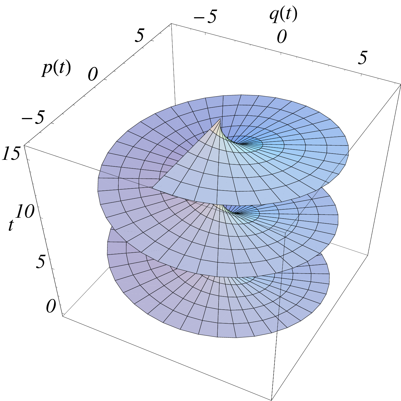
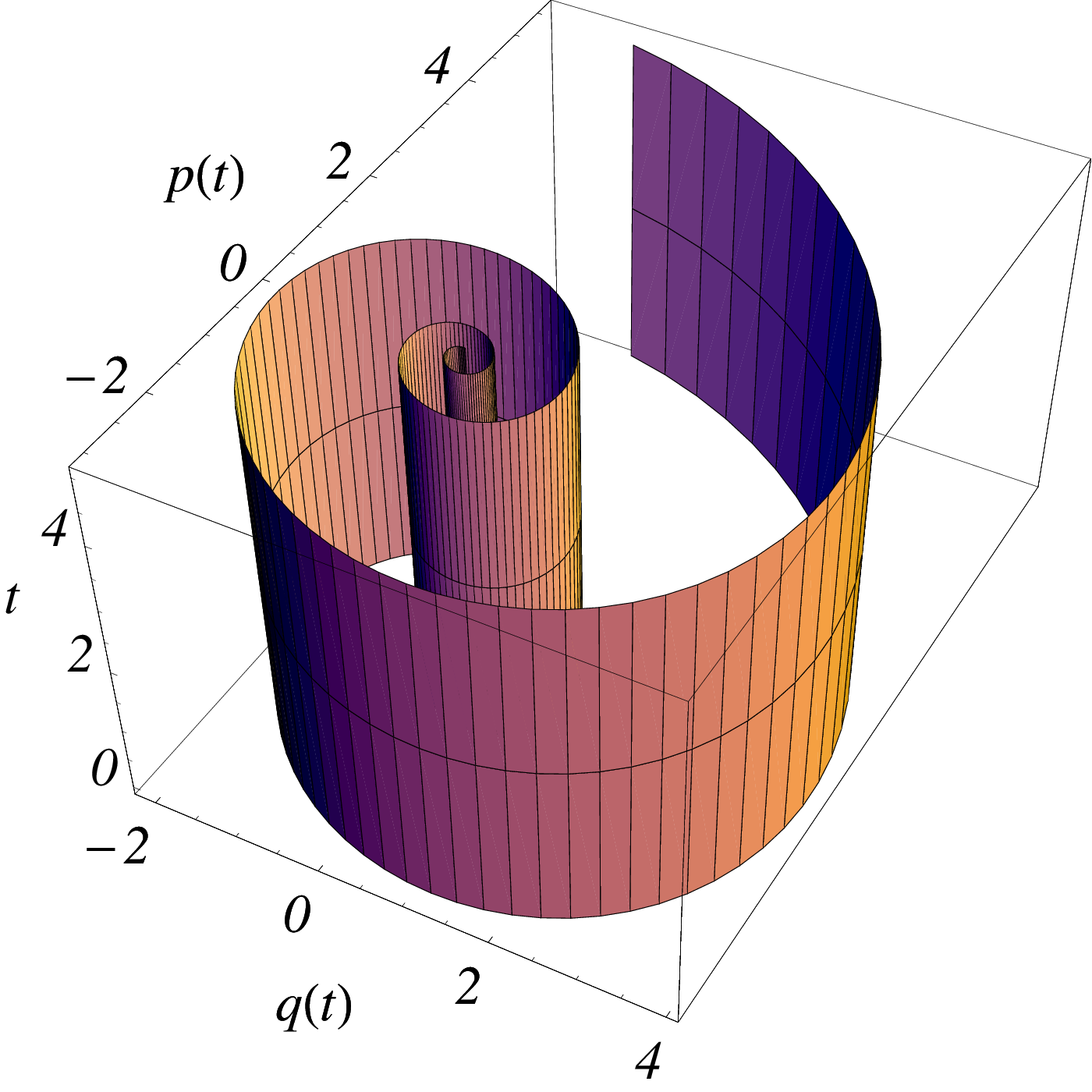
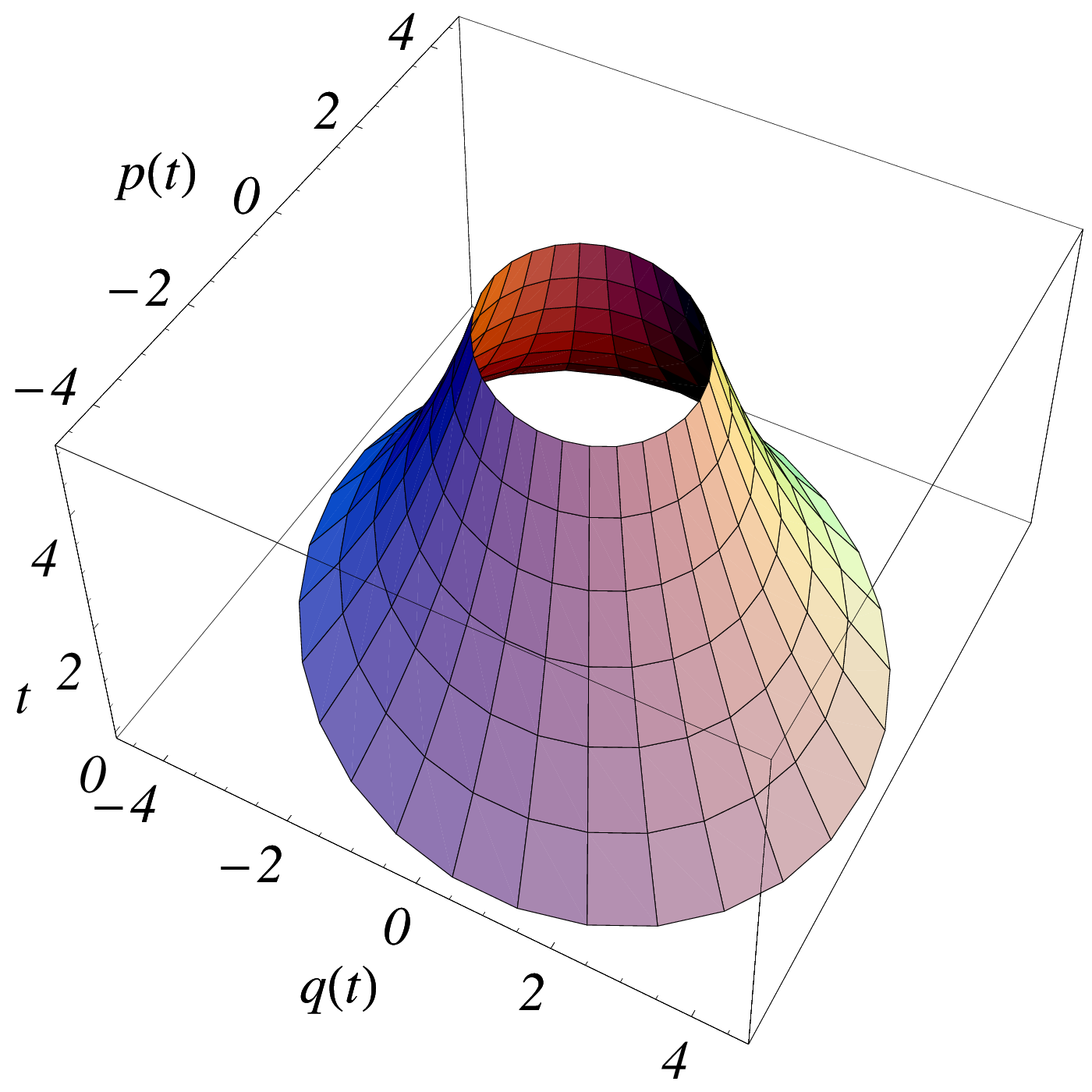
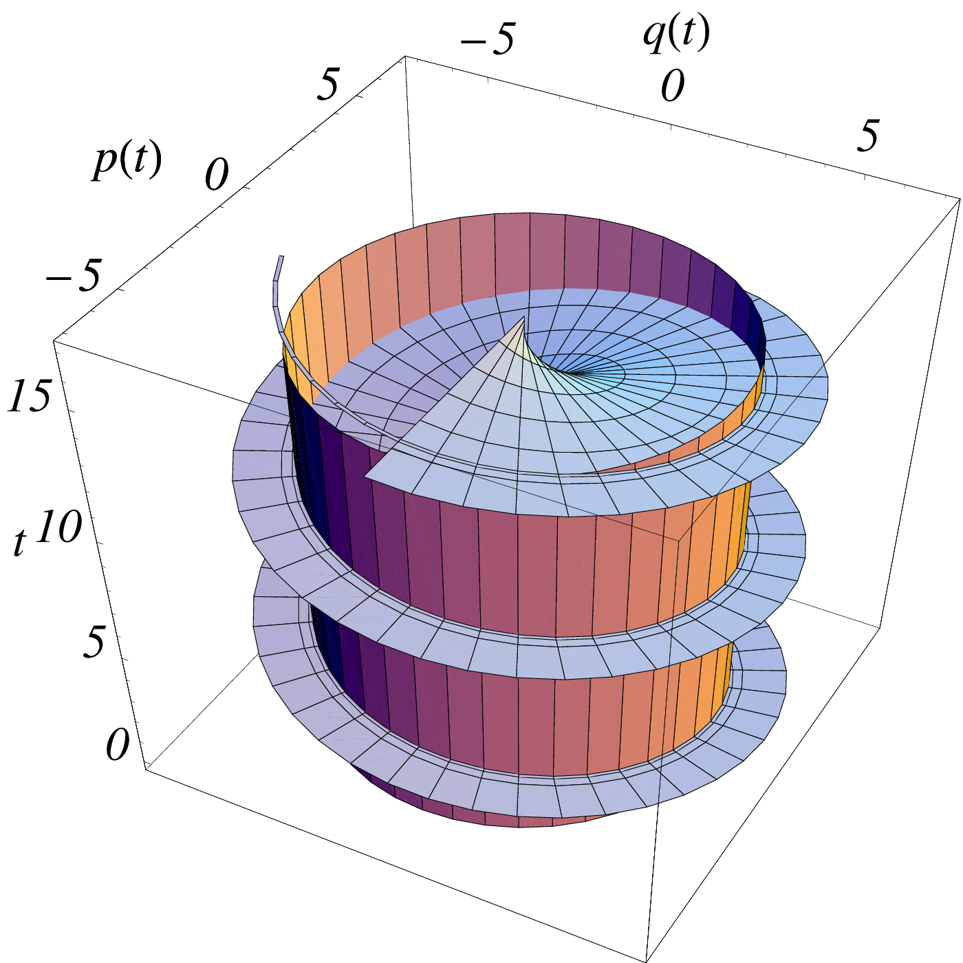
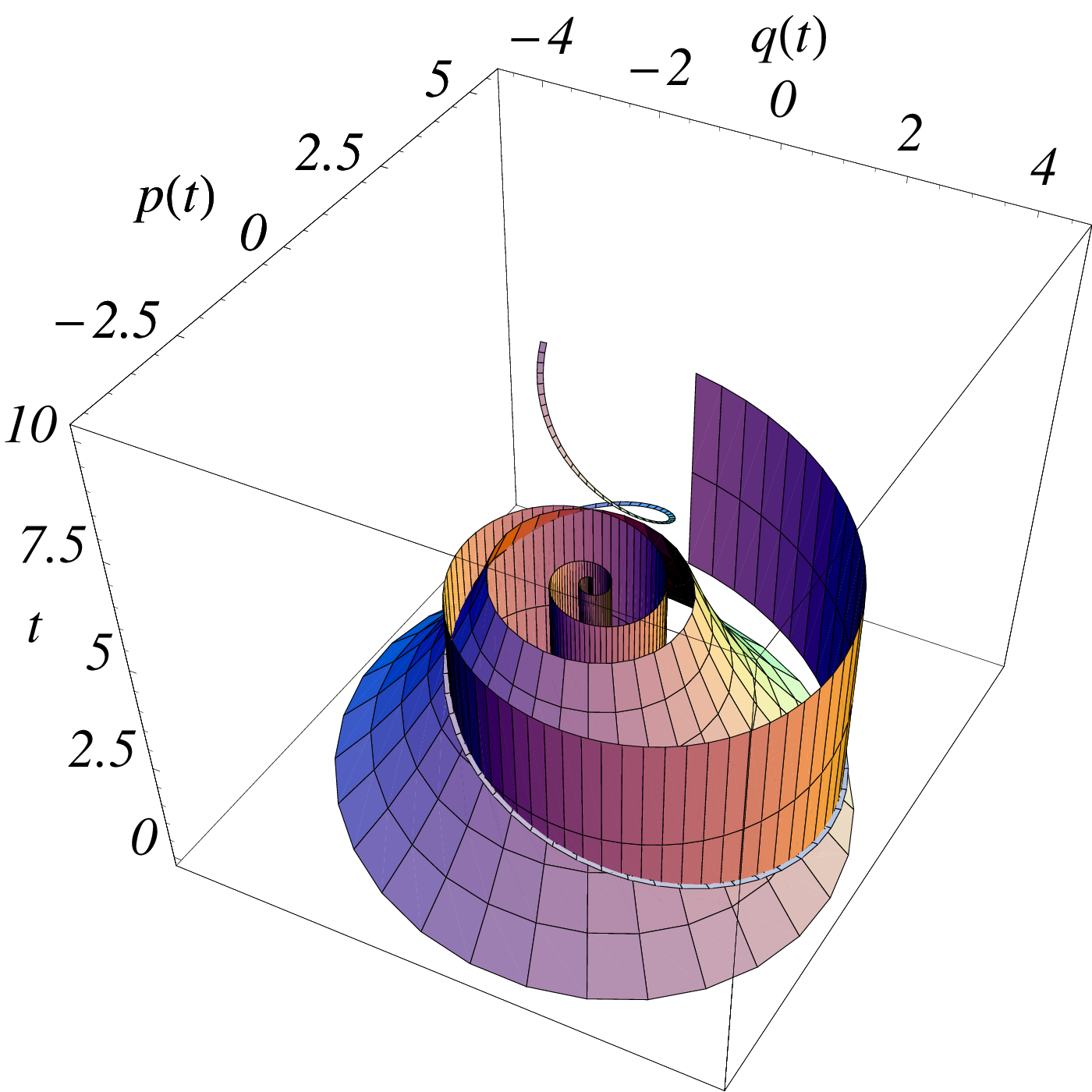
In Fig.4, upper panel, we show level surface of conservation law $E=30$ (on the left), level surface of dynamical invariant $T=0$ (middle) and solution trajectory $q(t),p(t)$ (on the right). This solution is actually the intersection of the level surfaces $E=30$ and $T=0$ ; for completeness of presentation, we show together the level surfaces and the solution in Fig.5 (left panel).

Notice that coordinates $q,p$ are not suitable for a global parametrization of dynamical invariant $T$ , (12), because $\arctan(x)$ is multi-valued. This problem can easily be overcome by using new coordinates $(R,\theta)$ :

q=R\sin\theta\,,\quad p=R\cos\theta

(14)

which allow us to rewrite $T$ as

T(q,p,t)=\tilde{T}(R,\theta,t)=t-\theta,

(15)

thereby eliminating the ambiguity. The plot of level surface $\tilde{T}=0$ in the middle upper panel of Fig.4 was done using the parameters $(R,t)$ .

2. Case $0<\alpha<2$ . Let $\alpha/2=\sin\varphi$ , then a dynamical invariant for the system is known:

D(q,p,t)=\left(p^{2}+q^{2}+2\,p\,q\sin\varphi\right)\exp(2\,t\sin\varphi).

(16)

We need to find a CL in order to determine the solution. Here we simply state the following CL:

	$\displaystyle C(q,p)$	$\displaystyle=$	$\displaystyle\frac{\cos\varphi}{2}\left(p^{2}+q^{2}+2\,p\,q\sin\varphi\right)$		(17)
		$\displaystyle\times$	$\displaystyle\exp{\Big[2\tan\varphi\arctan(\frac{q}{p}\sec\varphi+\tan\varphi)\Big]}.$		(17)

The method of construction of this CL is not important right now, it will be detailed in the next section. In Fig.4, lower panel, we show level surface of conservation law $C=30$ (on the left), level surface of dynamical invariant $D=20$ (middle) and solution trajectory $q(t),p(t)$ (on the right). This solution corresponds to the intersection of the level surfaces $C=30$ and $D=20$ ; for completeness, the level surfaces and the solution are shown together in Fig.5 (right panel).

Similar to the case of $\alpha=0$ dynamical invariant, the CL $C(q,p)$ is not globally defined. The following change of variables is needed:

q=R\,\sec\varphi\,\sin(\theta-\varphi),\quad p=R\,\cos\theta\,\sec\varphi,

(18)

in order to parameterize globally the CL. The result is

C(q,p)=\tilde{C}(R,\theta)=\frac{\cos\varphi}{2}R^{2}\exp(2\theta\tan\varphi).

(19)

It is important to realize that the two changes of variables (14) and (18) are suggested by the form of the respective invariants. Moreover, in the new variables $(R,\theta),$ both $T$ and $C$ take a simpler form (see (15),(19)). The reason for it is clear in the case $\alpha=0$ because $(R,\theta)$ are the well-known action-angle variables. In the general case, the variables $(R,\theta)$ determine a covering of the original variables.

The solution of the dynamical system is finally

	$\displaystyle q(t)$	$\displaystyle=$	$\displaystyle\frac{{\sqrt{D}}\,\sin(t\,\cos\varphi+\frac{1}{2}\log(\frac{C}{D})\cot\varphi-\varphi)}{\cos\varphi\,\exp({t\,\sin\varphi})}$		(20)
	$\displaystyle p(t)$	$\displaystyle=$	$\displaystyle\frac{{\sqrt{D}}\,\cos(t\,\cos\varphi+\frac{1}{2}\log(\frac{C}{D})\cot\varphi)}{\cos\varphi\,\exp({t\,\sin\varphi})}.$		(21)

III.2.2 Description of a laboratory experiment

To check the constancy of the conservation law $C(q,p)$ in a school laboratory experiment, we give here detailed description of the possible experiment in the case of sub-critical damping $0<\alpha<2$ . Moreover, we provide evidence of the practical and physical interest of the conservation law $C(q,p)$ : it can be used to measure the damping coefficient $\alpha$ . A simple pendulum oscillating at small amplitudes is easy to construct, consisting of a massive bob attached to the ceiling by a light (i.e. massless) string or rod. Damping can be easily introduced by attaching to the pendulum rod a sheet made of a light material. For small amplitudes, the angular frequency of the oscillations is given by $\omega=\sqrt{g/L}$ , where $g\approx 9.8[m/s^{2}]$ is the acceleration of gravity and $L$ is the pendulum length. We assume $\omega$ to be known, though of course it could be measured experimentally. From now on, we choose units where $\omega=1$ , so the damped pendulum equations for small amplitudes reduces to the system (10), where $q$ is the position of the oscillating bob and $p$ is its velocity.

With the aid of cheap electronic detection equipment it is possible to measure accurately the time $t$ , position $q$ and velocity $p$ of the oscillating bob at certain instances, namely when the bob passes near a detector. This data is sent to a computer database and analyzed with a software that comes along with the detection equipment. As a result one obtains a set of data points of the form

(q_{n},p_{n},t_{n})\,,\quad n=0,\ldots,N

(22)

With the aid of only one detector, we can in principle measure data at instances when $q_{n}=0$ . To wit, we first calibrate the detector by setting the $q=0$ coordinate as the equilibrium position of the mass. An experimental realization consists in producing a small amplitude oscillation and acquiring data points of the form (22). By looking at (18), these instances correspond to

\theta_{n}=\varphi+n\pi,\quad p_{n}=(-1)^{n}R_{n},

where $\varphi$ is the unknown parameter related to the damping coefficient by $\alpha=2\sin\varphi$ . From (19) we obtain data values

C_{n}=\frac{\cos\varphi}{2}p_{n}^{2}\exp(2(\varphi+n\pi)\tan\varphi).

If $C$ is a conservation law, then $C_{n}$ must be constant, independent of $n$ . Therefore we should have

p_{n}^{2}\exp(2n\pi\tan\varphi)=\mathop{\rm const}\nolimits=p_{0}^{2}.

In practice one can measure $\tan\varphi$ by finding a linear fit of $\log|p_{n}|$ versus $n$ :

\log|p_{n}|=\log|p_{0}|-n\pi\tan\varphi\,,\quad n=1,\ldots,N.

(23)

Once $\tan\varphi$ has been obtained, the damping coefficient $\alpha$ is readily computed.

Notice that one could use alternatively the dynamical invariant $D(q,p,t)$ to compute $\alpha$ , from the data (22). Setting $t_{0}=0,$ from (16) we obtain

D_{n}=p_{n}^{2}\exp(2t_{n}\sin\varphi)=\mathop{\rm const}\nolimits=p_{0}^{2}.

We can measure $\sin\varphi$ by finding a linear fit of $\log|p_{n}|$ versus $t_{n}$ :

\log|p_{n}|=\log|p_{0}|-t_{n}\sin\varphi\,,\quad n=1,\ldots,N.

(24)

Finally, notice that these two ways to measure the damping coefficient imply a third way: by comparing (23) and (24) we solve for the data times

t_{n}=n\pi/\cos\varphi\,,\quad n=1,\ldots,N.

In this case, a simple linear fit of $t_{n}$ as a function of $n$ will allow us to obtain $\varphi$ and thereby the damping coefficient $\alpha.$

III.2.3 Construction of conservation law

To illustrate the procedure of construction of a conservation law, we take as an example the sub-critically damped harmonic oscillator, i.e. (10) with $0<\alpha<2$ . Here $N=2$ and $\Delta^{1}=p,\quad\Delta^{2}=-q-\alpha p$ . The dynamical system is just $2$ -dimensional and we will write it as a vector $(\Delta^{1},\Delta^{2})^{T}$ . The Theorem requires the existence of a standard Liouville volume density $\rho(x^{1},x^{2})$ satisfying

(\rho\Delta^{1})_{,1}+(\rho\Delta^{2})_{,2}=0,

(25)

and does not require the knowledge of conservation laws. In general, a Liouville density, solution of (25), is interpreted as follows. A small region $\mathcal{R}(t)$ with a volume $V(t)$ in phase space $(x_{1},x_{2})$ , will evolve in time due to the dynamical system (10). Then, $\rho$ is defined in such a way that the product $\rho\,V(t)$ is conserved in time as $\mathcal{R}(t)$ evolves. For the harmonic oscillator, it is well known that the volume of $\mathcal{R}(t)$ is preserved, i.e., a constant function is a Liouville density. For the damped harmonic oscillator, a direct check shows that a Liouville density is $\rho(q,p)=\left(q^{2}+p^{2}+2\alpha\,q\,p\right)^{-1}.$ With this information we just need to solve (26) for $H$ :

\left(\begin{array}[]{cc}0&1\\ -1&0\\ \end{array}\right)\left(\begin{array}[]{c}H_{,1}\\ H_{,2}\\ \end{array}\right)=\left(\begin{array}[]{c}\rho\,\Delta^{1}\\ \rho\,\Delta^{2}\\ \end{array}\right).

(26)

The answer can be obtained by direct integration (see [4] for more details):

	$\displaystyle H(q,p)=-\left(\frac{q\,\alpha\,\arctan(\frac{2\,p+q\,\alpha}{{\sqrt{-\left(q^{2}\,\left(-4+{\alpha}^{2}\right)\right)}}})}{{\sqrt{-\left(q^{2}\,\left(-4+{\alpha}^{2}\right)\right)}}}\right)+$
	$\displaystyle+\frac{\log(p^{2}+q^{2}+p\,q\,\alpha)}{2}$		(27)

The conservation law $C(q,p)$ given by Eq.(17) is a function of $H$ , chosen for its nice form:

C=\frac{\cos\varphi}{2}\exp(2H).

IV Triad

As it was shown above, the notion of dynamical invariant is an important tool for constructing new physically relevant conservation laws that can afterwards be studied in a simple laboratory experiment. In this section we would like to use this approach to prove integrability of a complex triad with dynamical system (4). Of course, integrability of (4) is a well-known fact (e.g. [61]). However, the explicit solution of (4) is usually written for a particular case, namely, when the dynamical phase – a phase combination corresponding to the chosen resonance conditions – is either zero or constant ([44], p.132, Eq.(6.7); [54], p.156, Eq.(3.26.19), etc.).

On the other hand, it is well known that dynamical phases play a substantial role in the dynamics of resonant clusters, e.g. [58], and their effect can easily be observed in numerical simulations, [5]. This was our motivation for constructing first an explicit solution in the amplitude-phase presentation, for (28). Thus, (4) is used for a preliminary check of our method.

Another important point is the following. As it was shown in the papers [36, 37, 39], an elastic pendulum with suitably chosen parameters can be used as a mechanical model of a resonant triad, and the results can be applied for the description of large-scale motions in the Earth’s atmosphere. In fact, this simple mechanical model can be used for a laboratory study of dynamical characteristics of primary clusters in an arbitrary system with cubic Hamiltonian. This is why the explicit analytical formulas for all dynamically relevant parameters, given below, are important.

IV.1 Integrability

In this case the system can be reduced to $N=4$ (see [4] for more details), the Theorem on $(N-2)$ –integrability can be applied and we obtain the following CL:

H_{T}=\operatorname{Im}(B_{1}B_{2}B_{3}^{*})\,,

which is the canonical Hamiltonian for this case and can, of course, be written out directly. A dynamical invariant for this system was originally presented in [4], in terms of the three real roots $R_{1}<R_{2}<R_{3}$ of the cubic polynomial

x^{3}+x^{2}=2/27-(27H_{T}^{2}-

(I_{13}+I_{23})(I_{13}-2I_{23})(I_{23}-2I_{13}))/27(I_{13}^{2}-I_{13}I_{23}+I_{23}^{2})^{3/2}\,,

but these roots’ dependence on the coordinates or the CLs was not made explicit. Moreover, the explicit solution for the amplitudes $C_{j}$ and phases $\theta_{j}$ in the amplitude-phase representation $B_{j}=C_{j}\exp\left(i\theta_{j}\right)$ was not provided. Here we improve the form of dynamical invariant and also produce explicit and useful expressions for the full solution, based on the trigonometric representation of the three real roots in the so-called Casus Irreducibilis.

IV.2 Amplitude-phase representation

Sys.(4) in the standard amplitude-phase representation $B_{j}=C_{j}\exp(i\theta_{j})$ reads:

\displaystyle\begin{cases}\dot{C}_{1}=ZC_{2}C_{3}\cos\varphi,\\ \dot{C}_{2}=ZC_{1}C_{3}\cos\varphi,\\ \dot{C}_{3}=-ZC_{1}C_{2}\cos\varphi,\\ \dot{\varphi}=-Z\,H_{T}(C_{1}^{-2}+C_{2}^{-2}-C_{3}^{-2}).\end{cases}

(28)

where $\varphi=\theta_{1}+\theta_{2}-\theta_{3}$ is the dynamical phase. The conservation laws (II) do not change their form in the new variables:

I_{23}=C_{2}^{2}+C_{3}^{2},\ \ I_{13}=C_{1}^{2}+C_{3}^{2},

but the Hamiltonian $H_{T}$ reads now

H_{T}=C_{1}C_{2}C_{3}\sin\varphi.

(29)

Let us introduce new variables:

\rho=I_{23}/I_{13}

(30)

and $\alpha\in[0,\pi]$ defined by

\cos\alpha=\frac{\left(-2+3\,\rho+3\,{\rho}^{2}-2\,{\rho}^{3}\right)\,{{{I}_{13}}}^{3}-27\,{{{H}_{T}}}^{2}}{2\,{\left(1-\rho+{\rho}^{2}\right)}^{\frac{3}{2}}\,{{{I}_{13}}}^{3}}\,.

(31)

Notice that $|\cos\alpha|\leq 1$ for dynamically accessible system’s configurations. Indeed, the use of intermediate variables $p={2\,{\left(1-\rho+{\rho}^{2}\right)}^{\frac{3}{2}}}$ and $q=-2+3\,\rho+3\,{\rho}^{2}-2\,{\rho}^{3}\,,$ allows one to conclude immediately that $p\geq 0$ and $p\geq\left|q\right|\quad\forall\,\rho\,.$ Both inequalities become equalities if $\rho=0$ or $\rho=1.$ This yields

\left(H_{T}^{2}\right)_{\mathrm{max}}=\left(\frac{I_{13}}{3}\right)^{3}\left(p+q\right)\geq 0\,,\quad\mbox{for}\quad\cos\alpha=-1,

and

(\cos\alpha)_{\mathrm{max}}=q/p\leq 1\,,\quad\mbox{for}\quad H_{T}=0,

where $(H_{T}^{2})_{\mathrm{max}}$ and $(\cos\alpha)_{\mathrm{max}}$ are maximum values of $H_{T}^{2}$ and $\cos\alpha$ correspondingly.

Now, the solution of (28) is obtained in terms of Jacobian functions with modulus

\mu=\cos\left(\frac{\alpha}{3}+\frac{\pi}{6}\right)/\cos\left(\frac{\alpha}{3}-\frac{\pi}{6}\right)\,,

(32)

and period

T=\frac{{\sqrt{2}}\,3^{\frac{1}{4}}\,{K}\left(\mu\right)}{Z\,{\left(1-\rho+{\rho}^{2}\right)}^{\frac{1}{4}}\,{\sqrt{\cos(\frac{\alpha}{3}-\frac{\pi}{6})}}\,{\sqrt{{{{I}}_{13}}}}}\,,

(33)

where $K(\mu)$ is the complete elliptic integral of the first kind.

IV.3 Solutions for amplitudes

We present explicit expressions for the amplitude squares. The convention used here is that the amplitudes are positive, which is the generic situation when $H_{T}\neq 0\,.$ In this convention, when $H_{T}=0$ the individual phases have discontinuities in time to account for the amplitudes’ sign changes. The amplitude squares are proportional to the modes’ energies and can be of great use for physical applications:

\displaystyle\begin{cases}C_{1}^{2}(t)=-\mu\,\left(\frac{2K(\mu)}{Z\,T}\right)^{2}{{\mathbf{sn}^{2}}\left(2\,K(\mu)\,\frac{{(t-t_{0})}}{{T}},\mu\right)}\\ \quad\quad\quad+\frac{I_{13}}{3}\left({2-\rho}+2\,{\sqrt{1-\rho+{\rho}^{2}}}\,\cos\left(\frac{\alpha}{3}\right)\right)\,,\\ C_{2}^{2}(t)=-\mu\,\left(\frac{2K(\mu)}{Z\,T}\right)^{2}{{\mathbf{sn}^{2}}\left(2\,K(\mu)\,\frac{{(t-t_{0})}}{{T}},\mu\right)}\\ \quad\quad\quad+\frac{I_{13}}{3}\left({2\rho-1}+2\,{\sqrt{1-\rho+{\rho}^{2}}}\,\cos\left(\frac{\alpha}{3}\right)\right)\,,\\ C_{3}^{2}(t)=\mu\,\left(\frac{2K(\mu)}{Z\,T}\right)^{2}{{\mathbf{sn}^{2}}\left(2\,K(\mu)\,\frac{{(t-t_{0})}}{{T}},\mu\right)}\\ \quad\quad\quad+\frac{I_{13}}{3}\left({\rho+1}-2\,{\sqrt{1-\rho+{\rho}^{2}}}\,\cos\left(\frac{\alpha}{3}\right)\right)\,,\end{cases}

(34)

where $\mathbf{sn}(\cdot,\mu)$ is Jacobian elliptic function and $t_{0}$ is given in terms of the initial conditions for the amplitudes $C_{1}^{2}(0),C_{2}^{2}(0),C_{3}^{2}(0)$ and $t_{0}$ is defined by the initial conditions as:

t_{0}=\textrm{sign}(\cos\varphi(0))\,\frac{T}{2\,K(\mu)}\times F\left(\arcsin\sqrt{x_{0}},\mu\right)\,,

(35)

where

x_{0}=\frac{\cos\left(\frac{\alpha}{3}\right)}{\sqrt{3}\,\cos\left(\frac{\alpha}{3}+\frac{\pi}{6}\right)}+\frac{Z^{2}\,T^{2}\,(C_{3}^{2}(0)-C_{2}^{2}(0)-C_{1}^{2}(0))}{12\,\mu\,K(\mu)^{2}}

(36)

and $F(\cdot,\mu)$ is the elliptic integral of the first kind.

Notice that each equation in (34) is a sum of two terms where the left terms are time-dependent and the right terms are not. Each right term, for instance

\frac{I_{13}}{3}\left({2-\rho}+2\,{\sqrt{1-\rho+{\rho}^{2}}}\,\cos\left(\frac{\alpha}{3}\right)\right)

can be written explicitly as a function of conserved quantities $I_{13},\ I_{23},\ H_{T}$ (expressions for $\rho$ and $\alpha$ are given by (30),(31)) and is, therefore, defined by the initial conditions.

The same is true for $\mu$ and $T$ as it follows from (32) and (33). In particular, one can use the equations in (34) to determine the minimum and maximum accessible values of each amplitude (using the fact that $\mathbf{sn}^{2}$ oscillates between $0$ and $1$ ). The characteristic energy variation of any resonant mode $E_{mode},$ between these minimum and maximum values, has a very simple form: $E_{mode}(t)\sim\mathbf{sn}^{2}(k\,t,\mu).$

IV.4 Solution for dynamical phase

The dynamical phase satisfies an evolution equation:

\dot{\varphi}=-Z\,H_{T}(C_{1}^{-2}+C_{2}^{-2}-C_{3}^{-2}).

(37)

The solution for the dynamical phase cannot be obtained by simply replacing the solution for the amplitudes in the Hamiltonian $H_{T}=C_{1}C_{2}C_{3}\sin\varphi$ and solving for $\varphi$ . The reason is that non-zero $\varphi$ generically evolves between $0$ and $\pi$ , crossing the value $\varphi=\pi/2$ periodically. This implies that $\sin^{-1}$ is double-valued and thus it is not possible to obtain $\varphi$ in a unique way.

Another way to obtain the solution for dynamical phase might be integrating (37) in time, using the solution for the amplitude squares, (34), but this way is also rather involved. On the other hand, some simple considerations allow us to find an analytical expression for the dynamical phase. Indeed, let us rewrite (28), taking into account that $\frac{d}{dt}C_{1}^{2}=2C_{1}\dot{C}_{1}$ and $H_{T}=C_{1}C_{2}C_{3}\sin\varphi$ :

\frac{d}{dt}C_{1}^{2}=2ZC_{1}C_{2}C_{3}\cos\varphi=2ZH_{T}\cot\varphi\,.

This equation can be solved for $\varphi$ in each of the disjoint domains $(0,\pi)$ and $(-\pi,0)$ :

\varphi(t)=\textrm{sign}(\varphi(0))\,\mathrm{\mathbf{arccot}}\left(\frac{\textrm{sign}(\varphi(0))\,\frac{d}{dt}C_{1}^{2}}{2\,Z\,H_{T}}\right)\,,

using the convention that the function $\mathrm{\mathbf{arccot}}$ takes values on $(0,\pi).$ Using solution (34) together with the identity $\mathrm{\mathbf{sn}}^{\prime}(x,\mu)=\mathrm{\mathbf{cn}}(x,\mu)\mathrm{\mathbf{dn}}(x,\mu)$ we arrive at an explicit expression for the dynamical phase:

\varphi(t)=\textrm{sign}(\varphi_{0})\,\mathrm{\mathbf{arccot}}\left(-\frac{\mu}{|H_{T}|}\left(\frac{2K(\mu)}{Z\,T}\right)^{3}y\right)\,,

(38)

where

y=\mathrm{\mathbf{sn\,cn\,dn}}\left(2\,K(\mu)\,\frac{{(t-t_{0})}}{{T}},\mu\right)

and $\mathrm{\mathbf{sn\,cn\,dn}}(\cdot,\mu)\equiv\mathrm{\mathbf{sn}}(\cdot,\mu)\,\mathrm{\mathbf{cn}}(\cdot,\mu)\,\mathrm{\mathbf{dn}}(\cdot,\mu)\,.$

The restriction to the domain $\varphi\in(-\pi,0)\cup(0,\pi)$ is quite general: if $\varphi$ is initially in the domain $(n\,\pi,(n+1)\,\pi)\,,n\in\mathbb{Z},$ one can take $\varphi$ to either $(-\pi,0)$ or $(0,\pi)$ by an appropriate shift of $2\,m\,\pi\,,m\in\mathbb{Z}\,,$ without changing the evolution equations. Due to its special dynamics, the phase will remain in the domain where it was initially.

We can simplify (38) using nome $q$ of elliptic function defined as

q=\exp\left(-\pi\frac{K^{\prime}(\mu)}{K(\mu)}\right).

Since

	$\displaystyle\frac{2K(\mu)}{\pi}\mathbf{sn}\left(2\,K(\mu)\,\frac{{(t-t_{0})}}{{T}},\mu\right)=$
	$\displaystyle\frac{4}{\mu}\sum_{n=0}^{\infty}\frac{q^{(2n+1)/2}}{1-q^{2n+1}}\sin(2n+1)\pi\frac{{(t-t_{0})}}{{T}},$		(39)

one can compute $\mathrm{\mathbf{sn\,cn\,dn}}(x,\mu)$ using the fact that $\mathbf{sn}^{\prime}=\mathbf{cn\,dn}$ . Explicit expression would be then a product of two infinite sums [25] and can be rewritten as a Fourier series. Since the nome $q$ is an explicit function of the initial conditions, to have Fourier representations of our dynamical variables might be useful regarding approximate solutions.

IV.5 Dynamical invariant

Below we present a dynamical invariant for (28) which has been used for the constructing the solution (34). Recall that a dynamical invariant depends on time, amplitudes and phases: $S(t,C_{1},C_{2},C_{3},\varphi)$ , with the property that it is a constant along any solution of the dynamical system: $S(t,C_{1}(t),C_{2}(t),C_{3}(t),\varphi(t))=\mathrm{const.}\,\forall\,t\,.$ Generically, only local expressions can be obtained for a dynamical invariant, due to the multi-valuedness of the inverse functions involved. In this particular case, however, since we know the period of any trajectory, this multi-valuedness can be eliminated partially by patching appropriately local expressions yielding

	$\displaystyle S(t,C_{1},C_{2},C_{3},\varphi)=t-\left\lfloor\frac{2(t-t_{0})+T}{2\,T}\right\rfloor\,T$
	$\displaystyle+\,\frac{(-1)^{\left\lfloor\frac{2(t-t_{0})+T}{T}\right\rfloor}\,T}{2\,K(\mu)}\,F\left(\arcsin\sqrt{x_{t}},\mu\right)\,,$		(40)

where $\lfloor\cdot\rfloor$ is the floor function and $x_{t}$ can be obtained from the expression (36) for $x_{0}$ by substituting $C_{j}(t)$ instead of $C_{j}(0)$ , for all $j=1,2,3.$

This dynamical invariant satisfies $S(t,C_{1}(t),C_{2}(t),C_{3}(t),\varphi(t))=t_{0}\quad\forall t\,,$ where $t_{0}$ is given in equation (35), and is an improvement of the corresponding formula presented in [4].

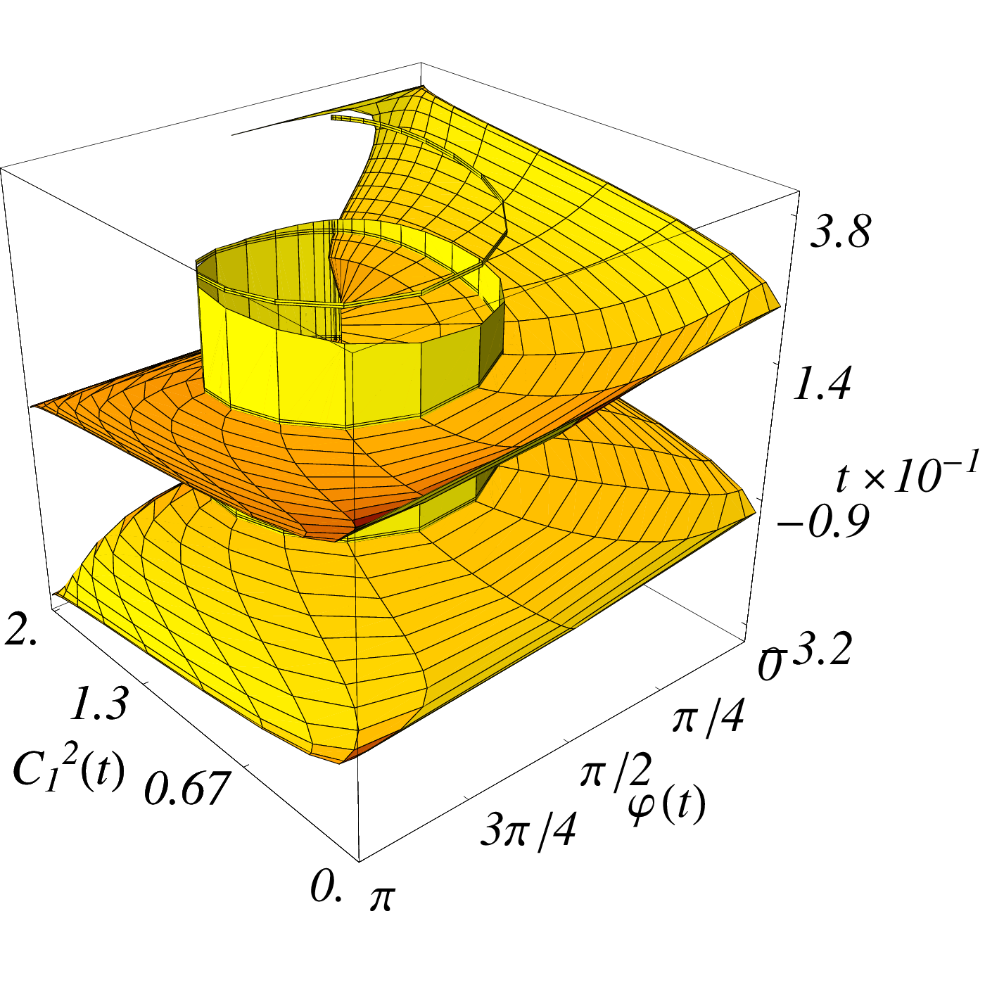
In Fig. 6, upper panel, we show, for fixed $I_{13}=2.00$ and $I_{23}=2.06$ : isosurface of conservation law $H_{T}=0.763$ , isosurface of dynamical invariant $S=2.69$ , solution trajectory and combined plot, in the domain $(C_{1},\varphi,t).$

In the middle of the upper panel, the surface $S=2.69$ is a helicoidal surface revolving around a vertical axis. This axis is the surface’s natural interior boundary: the constant-in-time trajectory corresponding to the highest possible value of $|H_{T}|$ for given $I_{13},I_{23}$ (obtained from the condition $\cos\alpha=-1$ ). In the present case, the highest possible value of $|H_{T}|$ is $1.114.$ This trajectory is physically interpreted as ‘maximum interference’, due to the fact that the modes do not interact. The dynamical phase is constant: $\varphi(t)=\pi/2\,\forall\,t,$ and all amplitudes are constant as well: from the condition $\mu=0$ and equations (34), we obtain in this case: $C_{1}^{2}(t)=1.33,\,\forall\,t\,.$ The exterior boundary of the surface is the piecewise continuous trajectory corresponding to the limit $H_{T}=0\,:$ in this limit the surface becomes non-differentiable at the ‘corners’ $C_{1}^{2}=0,I_{13},\,\varphi=0,\pi,$ due to the fact that the dynamical phase $\varphi$ is only piecewise continuous for $H_{T}=0$ . This trajectory corresponds to the usual case treated in textbooks, when amplitudes are considered real and individual phases vanish.

By looking at this figure we notice that the period $T$ decreases with increasing $H_{T}$ : the trajectories closer to the exterior boundary are more elongated than the trajectories closer to the interior boundary. In fact, from formula (33) one can prove this property analytically. In Fig. 7 we plot the period $T$ as a function of $H_{T}$ . We observe in this case a reduction of the period by a factor $0.5$ when $H_{T}$ is changed from 0 to $H_{\mathrm{max}}=1.114\,.$

In Fig. 6, lower panel, on the left and in the middle, combined plots are shown to clarify that the solution trajectory is the intersection of the isosurfaces of Hamiltonian and dynamical invariant. On the right, we show a combined plot of level surfaces of Manley–Rowe conservation laws $I_{13}$ , $I_{23}$ in the domain $(C_{1}^{2},C_{2}^{2},C_{3}^{2})$ .

IV.6 Special case $H_{T}=0$

Direct substitution shows that if we put $H_{T}=0$ , then new modulus and period take the form

\mu=\rho\quad\mbox{and}\quad T=\frac{2K(\rho)}{Z\sqrt{I_{13}}}

correspondingly, while the solutions for the amplitude squares read

\displaystyle\begin{cases}\tilde{C}_{1}^{2}(t)=\mathrm{dn}^{2}(\left(t-{t_{0}}\right)\,Z\,{\sqrt{{{{I}}_{13}}}},\rho)\,{{{{{{I}}}_{13}}}}\\ \tilde{C}_{2}^{2}(t)=\mathrm{cn}^{2}(\left(t-{t_{0}}\right)\,Z\,{\sqrt{{{{I}}_{13}}}},\rho)\,{{{{{{I}}}_{23}}}}\,\\ \tilde{C}_{3}^{2}(t)=\mathrm{sn}^{2}(\left(t-{t_{0}}\right)\,Z\,{\sqrt{{{{I}}_{13}}}},\rho)\,{{{{{{I}}}_{23}}}}\,.\end{cases}

(41)

As for the dynamical phase, from Eq.(38) it is seen that in the limit $H_{T}\to 0$ it behaves as a step function, jumping from $0$ to $\pi\,\mathrm{sign}(\varphi(0))$ :

\widetilde{\varphi}(t)=\frac{\pi\,\mathrm{sign}(\varphi(0))}{2}\left(1-(-1)^{\left\lfloor\frac{2(t-t_{0})}{T}\right\rfloor}\right)\,.

To understand the meaning of this behaviour, notice that the Hamiltonian $H_{T}$ is vanishing for $\varphi=n\,\pi,\,n\in\mathbb{Z}.$ The abrupt jumps of the dynamical phase is due to the jumps of the individual phases (solution not shown). These jumps replace the changes of sign of the modes’ amplitudes in the usual textbook descriptions.

As it was shown in [5], initial dynamical phase not in $\mathbb{Z}\,\pi$ substantially affects the magnitudes of resonantly interacting modes during the evolution, not only in a triad but also in a butterfly. This fact might have important implications (see [5], Discussion), for instance, for interpreting results of numerical simulations and for performing laboratory experiments.

V Generic clusters

It is well-known (see, for instance, [20, 22, 29, 30, KL-07, 33], etc.) that in three-wave resonance systems the most frequently met clusters are isolated triads or clusters consisting of two variously connected triads. Below we classify all possible two-triad clusters - kite, butterfly and ray - and show how to construct new CLs making use of the notion of dynamical invariant. In the last subsection, another method is briefly outlined which was presented in [59, 60] and allows one to prove, in some cases, integrability of bigger clusters.

V.1 Kite

A kite consists of two triads $a$ and $b,$ with wave amplitudes $B_{ja},\ B_{jb},$ $j=1,2,3$ , connected via two common modes. One can point out 4 types of kites according to the properties of connecting modes: PP-PP, AP-PP, AP-AP and AA-AA kites. In this section, PP-PP-kite with $B_{1a}=B_{1b}$ and $B_{2a}=B_{2b}$ is taken as a representative example. Its dynamical system reads:

\displaystyle\begin{cases}\dot{B}_{1a}=B_{2a}^{*}(Z_{a}B_{3a}+Z_{b}B_{3b})\,,\\ \dot{B}_{2a}=B_{1a}^{*}(Z_{a}B_{3a}+Z_{b}B_{3b})\,,\\ \dot{B}_{3a}=-Z_{a}B_{1a}B_{2a}\,,\ \dot{B}_{3b}=-Z_{b}B_{1a}B_{2a}\ .\end{cases}

(42)

It has 5 conservation laws (2 linear, 2 quadratic, 1 cubic):

\displaystyle\begin{cases}L_{R}=\operatorname{Re}(Z_{b}B_{3a}-Z_{a}B_{3b}),\ L_{I}=\operatorname{Im}(Z_{b}B_{3a}-Z_{a}B_{3b})\,,\\ I_{1ab}=|B_{1a}|^{2}+|B_{3a}|^{2}+|B_{3b}|^{2}\,,\\ I_{2ab}=|B_{2a}|^{2}+|B_{3a}|^{2}+|B_{3b}|^{2}\,,\\ H_{K}=\operatorname{Im}(Z_{a}B_{1a}B_{2a}B_{3a}^{*}+Z_{b}B_{1a}B_{2a}B_{3b}^{*})).\end{cases}

It has a dynamical invariant that is essentially the same as for a triad, $S$ , after replacing

Z=Z_{a}+Z_{b},\ \ H_{T}=H_{K}(Z_{a}^{2}+Z_{b}^{2})/Z^{3},

I_{13}=I_{1ab}(Z_{a}^{2}+Z_{b}^{2})/Z^{2}-(L_{R}^{2}+L_{I}^{2})/Z^{2},

I_{23}=I_{2ab}(Z_{a}^{2}+Z_{b}^{2})/Z^{2}-(L_{R}^{2}+L_{I}^{2})/Z^{2}.

V.2 Butterfly

A PP-butterfly consists of two triads $a$ and $b,$ with wave amplitudes $B_{ja},\ B_{jb},$ $j=1,2,3$ , and connecting mode, say $B_{1a}=B_{1b}=B_{1},$ is passive in both triads. The dynamical system for PP-butterfly reads

\displaystyle\begin{cases}\dot{B}_{1}=Z_{a}B_{2a}^{*}B_{3a}+Z_{b}B_{2b}^{*}B_{3b}\,,\\ \dot{B}_{2a}=Z_{a}B_{1}^{*}B_{3a}\,,\quad\dot{B}_{2b}=Z_{b}B_{1}^{*}B_{3b}\,,\\ \dot{B}_{3a}=-Z_{a}B_{1}B_{2a}\,,\ \dot{B}_{3b}=-Z_{b}B_{1}B_{2b}\ .\\ \end{cases}

(43)

We have studied this in [4]; we present here the results in order to compare the dynamics of different butterfly types and confirm the qualitative analysis given in [30]. Sys.(43) has 3 quadratic CLs analogous to (II) and 1 cubic CL corresponding to its Hamiltonian:

\displaystyle\begin{cases}I_{23a}=|B_{2a}|^{2}+|B_{3a}|^{2}\,,\quad I_{23b}=|B_{2b}|^{2}+|B_{3b}|^{2}\,,\\ I_{ab}=|B_{1}|^{2}+|B_{3a}|^{2}+|B_{3b}|^{2}\,,\\ H_{PP}=\operatorname{Im}(Z_{a}B_{1}B_{2a}B_{3a}^{*}+Z_{b}B_{1}B_{2b}B_{3b}^{*}).\end{cases}

(44)

Standard amplitude–phase representation. Here, one can rewrite the cubic conservation law as

H_{PP}=C_{PP}\left(Z_{a}C_{2a}C_{3a}\sin\varphi_{a}+Z_{b}C_{2b}C_{3b}\sin\varphi_{b}\right).

(45)

Here

\varphi_{a}=\theta_{1a}+\theta_{2a}-\theta_{3a},\quad\varphi_{b}=\theta_{1b}+\theta_{2b}-\theta_{3b}

are dynamical phases and $C_{(PP)}$ is the real amplitude of a common mode in PP-butterfly. This allows us to reduce Sys.(43) to only four real equations:

\displaystyle\begin{cases}\dot{C}_{3a}=-Z_{a}C_{PP}C_{2a}\cos\varphi_{a}\,,\\ \dot{C}_{3b}=-{Z_{b}}\,C_{PP}C_{2b}\cos\varphi_{b}\,,\\ \dot{\varphi}_{a}=-H_{PP}(C_{PP}^{-2}+C_{2a}^{-2}-C_{3a}^{-2}),\\ \dot{\varphi}_{b}=-H_{PP}(C_{PP}^{-2}+C_{2b}^{-2}-C_{3b}^{-2}).\end{cases}

(46)

Now the overall dynamics of the PP-butterfly is confined to a $3$ -dimensional manifold. The same can be done for the two other types of butterflies.

Modified amplitude-phase representation. The following change of variables was suggested in [4]:

\alpha_{a}=\arctan\left(C_{3a}/C_{2a}\right),\ \ \alpha_{b}=\arctan\left(C_{3b}/C_{2b}\right)\,.

with the inverse transformation being

\begin{cases}C_{2a}=\sqrt{I_{23a}}\cos\alpha_{a}\,,\quad C_{3a}=\sqrt{I_{23a}}\sin\alpha_{a}\,,\\ C_{2b}=\sqrt{I_{23b}}\cos\alpha_{b}\,,\quad C_{3b}=\sqrt{I_{23b}}\sin\alpha_{b}\,,\end{cases}

(47)

This change of variables allows further substantial simplification of (43) and (46):

\displaystyle\begin{cases}\dot{\alpha}_{a}=-Z_{a}C_{PP}\cos\varphi_{a},\\ \dot{\alpha}_{b}=-Z_{b}C_{PP}\cos\varphi_{b}\,,\\ \dot{\varphi}_{a}=Z_{a}C_{PP}\left(\cot\alpha_{a}-\tan\alpha_{a}\right)\sin\varphi_{a}-H_{PP}/C_{PP}^{2},\\ \dot{\varphi}_{b}={Z_{b}}C_{PP}\left(\cot\alpha_{b}-\tan\alpha_{b}\right)\sin\varphi_{b}-H_{PP}/C_{PP}^{2}.\end{cases}

(48)

In these new variables, the amplitude $C_{PP}>0$ reads

C_{PP}=\sqrt{I_{ab}-I_{23a}\sin^{2}\alpha_{a}-I_{23b}\sin^{2}\alpha_{b}}\,

(49)

and the Hamiltonian is now

	$\displaystyle H_{PP}=\frac{C_{PP}}{2}Z_{a}I_{23a}\sin{\varphi_{a}}\sin{2\alpha_{a}}+$
	$\displaystyle\frac{C_{PP}}{2}Z_{b}I_{23b}\sin{\varphi_{b}}\sin{2\alpha_{b}}.$		(50)

Eqs. (48)–(50) represent the final form of our three-dimensional general system in the modified amplitude-phase presentation.

A few cases of integrability in quadratures of the PP-butterfly were presented in [4]. The results are collected in Table 1 below. Of course, the form of the conservation laws is arbitrary in the sense that any set of functionally independent CLs will be suitable. For instance, in the case $H_{PP}=0$ we could choose the conserved quantity

A_{b}=\sin{\varphi_{b}}\sin{2\alpha_{b}}\quad\mbox{instead of}\quad A_{a}=\sin{\varphi_{a}}\sin{2\alpha_{a}}

(see Table 1, 1.2 PP) but not both because they are functionally dependent:

Z_{a}I_{23a}A_{a}+Z_{b}I_{23b}A_{b}\equiv 0.

Generally, we try to find the simplest presentation for our new constants of motion.

V.3 Ray

Analogously with the previous case, AA-butterfly is a two-triad cluster with a common mode which is A-mode in both triads, $B_{3a}=B_{3b}$ . Dynamical system and Manley–Rowe constants read:

	$\displaystyle\begin{cases}\dot{B}_{1a}=Z_{a}B_{2a}^{}B_{3a}\,,\ \dot{B}_{1b}=-Z_{b}B_{2b}^{}B_{3a}\,,\\ \dot{B}_{2a}=Z_{a}B_{1a}^{}B_{3a}\,,\quad\dot{B}_{2b}=Z_{b}B_{1b}^{}B_{3a}\,,\\ \dot{B}_{3a}=-Z_{a}B_{1a}B_{2a}-Z_{b}B_{1b}B_{2b}\ .\\ \end{cases}$		(51)
	$\displaystyle\begin{cases}I_{12a}=\|B_{1a}\|^{2}-\|B_{2a}\|^{2}\,,\quad I_{12b}=\|B_{1b}\|^{2}-\|B_{2b}\|^{2}\,,\\ I_{ab}=\|B_{1a}\|^{2}+\|B_{3a}\|^{2}+\|B_{3b}\|^{2}\ .\end{cases}$		(52)

The integrability of (51) can be investigated along the same lines as for (43) above. The analysis is omitted here. We just partly outline one particular case of this cluster: $AA$ -ray, which can be regarded as a degenerate $AA$ -butterfly, so that $\omega_{1b}=\omega_{2b}=\omega_{3}/2$ .

In this case, the dynamical system obtained from first principles will have the form

\displaystyle\begin{cases}\dot{B}_{1a}=Z_{a}B_{2a}^{*}B_{3}\,,\ \dot{B}_{b}=Z_{b}B_{b}^{*}B_{3}\,,\\ \dot{B}_{2a}=Z_{a}B_{1a}^{*}B_{3}\,,\quad\dot{B}_{3}=-Z_{a}B_{1a}B_{2a}-2Z_{b}B_{b}^{2}\ .\end{cases}

(53)

Notice that there is a factor $2$ in the last term of last equation, which would not appear if we made the direct substitution $B_{1b}=B_{2b}=B_{b}$ into system (51). Rather, the simple change of variables $B_{1b}=B_{2b}=\sqrt{2}B_{b}$ will transform the AA-butterfly (51) into the ray equations (53). This means in particular that integrable cases of AA-butterfly can be directly mapped to some integrable cases of AA-ray. Another interesting point is that AA-ray cluster might also have a nice mechanical model - Wilberforce pendulum [38], the problem is presently under the study.

Conservation laws for AA-ray are inherited from conservation laws for AA-butterfly:

\displaystyle\begin{cases}I_{12a}=|B_{1a}|^{2}-|B_{2a}|^{2}\,,\\ I_{ab}=|B_{1a}|^{2}+2|B_{b}|^{2}+|B_{3}|^{2}\ \,,\\ H_{\mathrm{ray}}=\operatorname{Im}(-Z_{a}B_{1a}B_{2a}B_{3}^{*}-2Z_{b}B_{b}^{2}B_{3}^{*}),\end{cases}

(54)

with dynamical phases

\varphi_{a}=\theta_{1a}+\theta_{2a}-\theta_{3},\quad\varphi_{b}=2\theta_{b}-\theta_{3}.

This reduces four complex equations (53) to only four real ones:

\displaystyle\begin{cases}\dot{C}_{1a}=Z_{a}C_{2a}C_{3}\cos\varphi_{a}\,,\\ \dot{C}_{b}={Z_{b}}C_{b}C_{3}\cos\varphi_{b}\,,\\ \dot{\varphi}_{a}=-Z_{a}C_{3}\left(\frac{C_{2a}}{C_{1a}}+\frac{C_{1a}}{C_{2a}}\right)\sin\varphi_{a}+H_{\mathrm{ray}}/C_{3}^{2}\\ \dot{\varphi}_{b}=-2Z_{b}C_{3}\sin\varphi_{b}+H_{\mathrm{ray}}/C_{3}^{2}\,,\end{cases}

(55)

with Hamiltonian

H_{\mathrm{ray}}=-C_{3}\left(Z_{a}C_{1a}C_{2a}\sin\varphi_{a}+2Z_{b}C_{b}^{2}\sin\varphi_{b}\right)

(56)

in terms of the amplitudes and phases.

Consider the simple case when initially $\varphi_{a}=\varphi_{b}=0$ . Then $H_{\mathrm{ray}}=0$ , phases remain zero for all times, and the equations of motion reduce to

\displaystyle\begin{cases}\dot{C}_{1a}=Z_{a}C_{2a}C_{3}\,,\\ \dot{C}_{2a}=Z_{a}C_{1a}C_{3}\,,\\ \dot{C}_{b}={Z_{b}}C_{b}C_{3}\,,\\ \dot{C}_{3}=-{Z_{a}}C_{1a}C_{2a}-2{Z_{b}}C_{b}^{2}\,.\end{cases}

(57)

with two Manley–Rowe constants of motion

\displaystyle\begin{cases}I_{12a}=C_{1a}^{2}-C_{2a}^{2}\,,\\ I_{ab}=C_{1a}^{2}+2C_{b}^{2}+C_{3}^{2}\ \,.\end{cases}

(58)

and a new one

\displaystyle H_{\mathrm{new}}=2Z_{a}\ln C_{b}+Z_{b}\ln\left(\frac{C_{2a}-C_{1a}}{C_{2a}+C_{1a}}\right)\,,

(59)

where notations

C_{1a}=\sqrt{I_{12a}}\cosh\alpha\,,\quad C_{2a}=\sqrt{I_{12a}}\sinh\alpha

are used.

Notice that this way only non-polynomial additional conservation laws are obtained (see Table 1).

Conditions		Additional CLs
$\varphi_{a}=\varphi_{b}=0$	1.1.	$Z_{b}\arctan\left(\frac{C_{3a}}{C_{2a}}\right)-Z_{a}\arctan\left(\frac{C_{3b}}{C_{2b}}\right)$
	PP-but.
$\varphi_{a},\ \varphi_{b}\neq 0,\ H_{PP}=0$	1.2.	$A_{a}=\sin{\varphi_{a}}\sin{2\alpha_{a}},$ with $\alpha_{a}=\arctan\left(C_{3a}/C_{2a}\right)$
	PP-but.
	1.3.	$(1+\frac{Z_{b}}{Z_{a}})\arccos\left(\frac{\cos 2\alpha_{a}}{\sqrt{1-A_{a}^{2}}}\right)-(1+\frac{Z_{b}}{Z_{a}})\arccos\left(\frac{\cos 2\alpha_{b}}{\sqrt{1-A_{b}^{2}}}\right)$
	PP-but.
		with $\alpha_{b}=\arctan\left(C_{3b}/C_{2b}\right)$ and $A_{b}=\sin{\varphi_{b}}\sin{2\alpha_{b}}$
$H_{PP}\neq 0,\ Z_{a}=Z_{b}$	1.4.	$C_{2a}^{2}C_{3a}^{2}+C_{2b}^{2}C_{3b}^{2}+2C_{2a}C_{3a}C_{2b}C_{3b}\cos(\varphi_{a}-\varphi_{b})-C_{1}^{2}(C_{1}^{2}-C_{2a}^{2}+C_{3a}^{2}-C_{2b}^{2}+C_{3b}^{2})$
	PP-but.
	2.1.	$2Z_{a}\ln C_{b}+Z_{b}\ln\Big[(C_{2a}-C_{1a})/(C_{2a}+C_{1a})\Big]$
$\varphi_{a}=\varphi_{b}=0$	AA-ray	with $C_{1a}=\sqrt{I_{12a}}\cosh\alpha\,,\quad C_{2a}=\sqrt{I_{12a}}\sinh\alpha\,,\quad I_{12a}=C_{1a}^{2}-C_{2a}^{2}$

Table 1: Examples of non-polynomial conservation laws.

V.4 Star

A cluster of N triads, all connected via one common mode is called N-star cluster. Again, integrability of N-star depends on the types these connecting modes have in each triad of a cluster. NR-diagrams for all possible types of 3-stars are shown in Fig. 11.

N-star cluster is probably the only presently known type of cluster for which an analytical study has been performed for arbitrary finite number $N$ . The main idea can be briefly formulated as follows. N-star cluster has 2N+1 degrees of freedom, N+1 Manley–Rowe constants of motion and one Hamiltonian, that is, we already have N+2 independent first integrals in involution. To find $N-1$ additional integrals of motion, one can use construction of Lax operators, Painlevé analysis and irreducible forms (see [45, 46, 59, 60], etc.; terminology used therein is pump and daughter wave for A- and P-mode correspondingly). The dynamical system, say for N-star-A, is regarded in the form

	$\displaystyle\dot{B}_{1j}=i\,\lambda_{j}B_{3}\dot{B}_{2j},\quad\dot{B}_{2j}=i\,\lambda_{j}B_{3}\dot{B}_{1j},$		(60)
	$\displaystyle\dot{B}_{3}=i\,\sum_{j=1}^{N}\lambda_{j}B_{1j}B_{2j}.$		(61)

Additional conservation laws found this way have necessarily polynomial form. The results for a generic N-star cluster are as follows: N-star-A (with all A-connections) and N-star-P (with all P-connections) are integrable for arbitrary initial conditions if

\lambda_{j}=\frac{1}{2}\quad\mbox{or}\quad 1\quad\mbox{or}\quad 2,

examples of corresponding NR-diagrams shown in the Fig.11, upper panel, for $N=3$ . $N$ -star cluster with mixed A- and P-connections (Fig.11, lower panel) has no additional polynomial conservation laws. Complete set of additional polynomial conservation laws for integrable N-star cluster is omitted here for sake of place, and it can be found in [60]. Example for the case of AA-butterfly with $Z_{a}=2\,Z_{b}$ reads

	$\displaystyle 4(B_{1}B_{2}B_{4}^{}B_{5}^{}+B_{1}^{}B_{2}^{}B_{4}B_{5})(B_{1}B_{1}^{}+B_{2}B_{2}^{})$
	$\displaystyle-2(B_{3}B_{1}^{}B_{2}^{}+B_{3}^{}B_{1}B_{2})^{2}-[(B_{1}B_{1}^{}+B_{2}B_{2}^{*})^{2}$
	$\displaystyle+4B_{1}B_{1}^{}B_{2}B_{2}^{}](B_{4}B_{4}^{}+B_{5}B_{5}^{}).$		(62)

The general way to investigate integrability of a generic cluster would be to apply the theory of normal forms (see, for instance, [50, 52]) for each dynamical system describing a resonance cluster is a normal form. But of course, most generic clusters demonstrate chaotic behavior and numerical investigations are unavoidable.

Here we outline briefly which facts are important in order to perform sensible numerical simulations with resonance clusters. The fact that our systems are Hamiltonian, allows us to perform numerical simulations based on the Hamiltonian expansion of the corresponding dynamical system. Poincaré sections are well-known instruments to show clearly whether or not a dynamical system demonstrates chaotic behavior, so all the results of our numerical simulations are illustrated by the corresponding Poincaré maps. One of the most tedious and time-consuming parts of the corresponding simulations is the choice of initial conditions. A special procedure has been worked out [43] that guarantees a uniform distribution of initial conditions according to Liouville measure, and assures as well that all conservation laws have the same value on each Poincaré section. In Fig.12 an example of Poincaré section is shown.

To trace effects due to the dynamical phases one has to use amplitude-phase representations, of course.

VI Coupling coefficient

As we have shown above, the integrability of a resonance cluster depends on the magnitude of the corresponding coupling coefficients. Expressions for coupling coefficients in canonical variables has been deduced for various types of wave systems possessing three-wave resonances: irrotational capillary waves [66]; rotational capillary waves [10]; irrotational gravity-capillary waves [47]; rotational gravity-capillary waves [18], drift waves [56], etc. They usually have a nice compact form, for instance, coupling coefficient $V^{3}_{12}$ for irrotational gravity-capillary water waves reads

\frac{(\omega_{2}^{2}-\omega_{2}\omega_{3}+\omega_{3}^{2})}{\omega_{1}}k_{1}-\omega_{2}k_{2}+\omega_{3}k_{3},

where $\omega=(g\,k+\sigma k^{3})^{1/2}$ and $g$ and $\sigma$ are gravity acceleration and surface tension correspondingly. However, transformation of these expressions from the canonical to physical variables is not an easy task.

On the other hand, the application of multi-scale methods yields expressions for the coupling coefficients directly in physical variables. For instance, coupling coefficients of the system of three resonantly interacting atmospheric planetary waves, with $\omega\sim m/[n(n+1)]$ , have the form [33]

\displaystyle\begin{cases}Z[n_{2}(n_{2}+1)-n_{3}(n_{3}+1)]/[n_{1}(n_{1}+1)],\\ Z[n_{3}(n_{3}+1)-n_{1}(n_{1}+1)]/[n_{2}(n_{2}+1)],\\ Z[n_{2}(n_{2}+1)-n_{1}(n_{1}+1)]/[n_{3}(n_{3}+1)],\end{cases}

(63)

with

Z=\int_{-\pi/2}^{\pi/2}[m_{2}P^{(2)}\frac{d}{d\varphi}P^{(1)}-m_{1}P^{(1)}\frac{d}{d\varphi}P^{(2)}]\frac{d}{d\varphi}P^{(3)}d\varphi.

Here two spherical space variables are the latitude $\varphi$ , $-\pi/2\leq\varphi\leq\pi/2$ , and the longitude $\lambda$ , $0\leq\lambda\leq 2\pi$ , and the notation $P^{(j)}$ is used for $P_{n_{j}}^{m_{j}}(\sin\varphi)$ which is the associated Legendre function of degree $n_{j}$ and order $m_{j}$ .

The multi-scale method is quite straightforward and can be programmed in some symbolical language [33]. However, only numerical magnitudes of the coupling coefficients have been computed for selected solutions of the resonance conditions, not an explicit algebraic formulas. The problem is due to some ”bags” in Mathematica in computing integrals of the form

\int_{0}^{2\pi}\sin(mx)\sin(nx)dx,\quad\mbox{with}\quad m,n\in\mathbb{N},

(64)

more discussion can be found in [33].

For completeness of presentation we show below a part of the formula for one coupling coefficient, obtained by a combination of symbolical programming in Mathematica and automatic search-and-replace of formulas of the type (64) – which Mathematica cannot handle directly – for ocean planetary waves with vanishing boundary conditions, $\omega\sim(m^{2}+n^{2})^{-1/2}$ , in physical variables. The general form of the coupling coefficients is

\alpha_{j}/[(m_{j}^{2}+n_{j}^{2})\pi^{2}],\quad j=1,2,3,

(65)

with coefficients $\alpha_{j}$ being functions of the wavenumbers $m_{1},\,n_{1},\,\cdots,m_{3},\,n_{3}.$ Notations E and I below are for exponent $\exp$ and imaginary unit $i$ , all other notations are self-explanatory. Notation (…) at the end is used for eight more pages, needed to accomplish this formula.

$\alpha_{1}=\frac{1}{16}\times$

(E^(-I (m1 + m2 + m3 + Sqrt[m1^2 + n1^2] + Sqrt[m2^2 + n2^2] - Sqrt[m3^2 +n3^2])\[Pi])
((I (m2^2 m3 n2 - 2 m3^3 n2 + m3 n2^3 + m2 m3 n2 Sqrt[m2^2 + n2^2] + 2 m2^3 n3 - m2 m3^2 n3
+ 2 m2 n2^2 n3 + 2 m2^2 Sqrt[m2^2 + n2^2] n3 - m3^2 Sqrt[m2^2 + n2^2] n3 + n2^2 Sqrt[m2^2
+ n2^2] n3 - 2 m3 n2 n3^2 - m2 n3^3 - Sqrt[m2^2 + n2^2] n3^3 + m2^2 n2 Sqrt[m3^2 + n3^2]
- 2 m3^2 n2 Sqrt[m3^2 + n3^2] + n2^3 Sqrt[m3^2 + n3^2] + m2 n2 Sqrt[m2^2 + n2^2] Sqrt[m3^2
+ n3^2] - m2 m3 n3 Sqrt[m3^2 + n3^2] - m3 Sqrt[m2^2 + n2^2] n3 Sqrt[m3^2 + n3^2]
- n2 n3^2 Sqrt[m3^2 + n3^2]))/(m1 + m2 - m3 + Sqrt[m1^2 + n1^2] + Sqrt[m2^2 + n2^2]
- Sqrt[m3^2 + n3^2]) + (I (m2^2 m3 n2 - 2 m3^3 n2 + m3 n2^3 + m2 m3 n2 Sqrt[m2^2 + n2^2]
+ 2 m2^3 n3 - m2 m3^2 n3 + 2 m2 n2^2 n3 + 2 m2^2 Sqrt[m2^2 + n2^2] n3 - m3^2 Sqrt[m2^2
+ n2^2] n3 + n2^2 Sqrt[m2^2 + n2^2] n3 - 2 m3 n2 n3^2 - m2 n3^3 - Sqrt[m2^2 + n2^2] n3^3
+ m2^2 n2 Sqrt[m3^2 + n3^2] - 2 m3^2 n2 Sqrt[m3^2 + n3^2] + n2^3 Sqrt[m3^2 + n3^2]
+ m2 n2 Sqrt[m2^2 + n2^2] Sqrt[m3^2 + n3^2] - m2 m3 n3 Sqrt[m3^2 + n3^2] - m3 Sqrt[m2^2
+ n2^2] n3 Sqrt[m3^2 + n3^2] - n2 n3^2 Sqrt[m3^2 + n3^2]))/(m1 - m2 + m3 - Sqrt[m1^2
+ n1^2] - Sqrt[m2^2 + n2^2] + Sqrt[m3^2 + n3^2]) - (I (m2^2 m3 n2 - 2 m3^3 n2 + m3 n2^3
- (...)

VII Summary

(..to be added: numerical simulations, NR-reduced models..)

Acknowledgements. The authors are very much obliged to the organizing committee of the workshop “INTEGRABLE SYSTEMS AND THE TRANSITION TO CHAOS II,” who provided an excellent opportunity to meet and work together. They also highly appreciate the hospitality of Centro Internacional de Ciencias (Cuernavaca, Mexico), where part of the work was accomplished. Authors would like to thank A. Degasperis, S. Lombardi and F. Leyvraz for interesting and fruitful discussions. M.B. acknowledge the support of the Transnational Access Programme at RISC-Linz, funded by European Commission Framework 6 Programme for Integrated Infrastructures Initiatives under the project SCIEnce (Contract No. 026133). E.K. acknowledges the support of the Austrian Science Foundation (FWF) under project P20164-N18 “Discrete resonances in nonlinear wave systems”.

References

[1] Almonte, F., V.K. Jirsa, E.W. Large and B. Tuller. Physica D 212 (1-2): 137 (2005)
[2] Arnold, V.I. Geometrical Methods in the Theory of Ordinary Differential Equations. Grundleheren der mathematischen Wissenschaften 250 (A Series of Comprehensive Studies in Mathematics) New York Heidelberg Berlin: Springer-Verlag (1983)
[3] Bolsinov, A.V., and A.T. Fomenko. Integrable Hamiltonian Systems, Chapmann $\&$ Hall/CRC (2004)
[4] Bustamante, M.D., and E. Kartashova. Europhys. Lett. 85: 14004 (2009)
[5] Bustamante, M.D., and E. Kartashova. Europhys. Lett., 85: 34002 (2009)
[6] Calogero, F. In book: V.E. Zakharov (ed.) What is Integrability?: 1 (1991) (Springer Series in Nonlinear Dynamics, Springer Verlag)
[7] Chow, C. C., D. Henderson and H. Segur. Fluid Mech., 319: 67 (1996)
[8] Cretin, B., and D. Vernier. E-print: arxiv.org/abs/0801.1301 (2008)
[9] Constantin, A., and E. Kartashova. EPL, 86: 29001 (2009)
[10] Constantin, A., E. Kartashova and E. Wahlén. E-print: arXiv:1001.1497 (2010)
[11] Denissenko, P., S. Lukaschuk and S. Nazarenko, Phys. Rev. Lett., 99: 014501 (2007)
[12] Dubrovin, B., and Y. Zhang. E-print: arXiv:math/0108160v1 (2001)
[13] Eissa, M., W.A.A. El-Ganainia and Y.S. Hameda. Physica A: Stat. Mech. Appl. 356(2-4): 341 (2005)
[14] Evans, N.W. Phys. Rev. A 41 (10): 5566 (1990)
[15] Haenggi, P. ChemPhysChem 3 (3): 285 (2002)
[16] Hasselmann, K. Fluid Mech 30: 737 (1967)
[17] Horvat, K., M. Miskovic and O. Kuljaca. Industrial Technology 2: 881 (2003)
[18] Johnson, R. S. A Modern Introduction to the Mathematical Theory of Water Waves (Cambridge University Press, 1997)
[19] Kartashova, E.A., L.I. Piterbarg and G.M. Reznik. Oceanology, 29: 405 (1990)
[20] Kartashova, E. Phys. Rev. Lett. 72: 2013 (1994)
[21] Kartashova, E. AMS Transl. 2: 95 (1998)
[22] Kartashova, E. JETP Lett. 83(7): 341 (2006)
[23] Kartashova, E. Low Temp. Phys. 145 (1-4): 286 (2006)
[24] Kartashova, E. Phys. Rev. Lett. 98(21): 214502 (2007)
[25] Kartashova, E. Europhys. Lett., 87: 44001 (2009)
[26] Kartashova, E. Nonlinear Resonance Analysis: Theory, Computation, Applications (Cambridge University Press, 2010, in press)
[27] Kartashova, E., and A. Kartashov. Int. J. Mod. Phys. C 17(11): 1579 (2006)
[28] Kartashova, E., and A. Kartashov. Comm. Comp. Phys. 2(4): 783 (2007)
[29] Kartashova, E., and A. Kartashov. Physica A: Stat. Mech. Appl. 380: 66 (2007)
[30] Kartashova, E., and V.S. L’vov. Phys. Rev. Lett. 98(19): 198501 (2007)
[31] Kartashova, E., and V.S. L’vov. Europhys. Lett. 83: 50012 (2008)
[32] Kartashova, E., and G. Mayrhofer. Physica A: Stat. Mech. Appl. 385: 527 (2007)
[33] Kartashova, E., C. Raab, Ch. Feurer, G. Mayrhofer and W. Schreiner. In: Extreme Ocean Waves: 97. Eds: E. Pelinovsky and Ch. Harif, Springer (2008)
[34] Kartashova, E., and A. Shabat. RISC Report Series, N0002-04-2005 (2005).
[35] Karuzskii, A.L., A.N. Lykov, A.V. Perestoronin and A.I. Golovashkin. Physica C: Superconductivity 408-410: 739 (2004)
[36] P. Lynch. Int. J. Nonl. Mech. 37: 258 (2002)
[37] P. Lynch. In: Large-Scale Atmosphere-Ocean Dynamics: Vol II: Geometric Methods and Models: 64. Eds. J. Norbury and I. Roulstone (Cambridge University Press, 2002)
[38] P. Lynch, private communication (2009).
[39] P. Lynch, and C. Houghton, Physica D 190: 38 (2004)
[40] Oliveira, H.P. de, I. Damia o Soares and E.V. Tonini Cosmology and Astroparticle Physics, doi: 10.1088/1475-7516/2006/02/015
[41] Kovriguine, D.A., and G.A. Maugin Mathematical Problems in Engineering, doi:10.1155/MPE/2006/76041 (2006)
[42] Kundu, M., and D. Bauer. Phys. Rev. Lett. 96: 123401 (2006)
[43] F. Leyvraz (personal communication, 2008)
[44] Longuet-Higgins, M.S., and Gill, A.E. , Resonant interactions between planetary waves. Proc. Roy. Soc. Lond. A299, 120 (1967)
[45] C. R. Menyuk, H. H. Chen and Y. C. Lee. Restricted multiple three-wave interactions: Panlevé analysis. Phys. Rev. A 27: 1597 (1983)
[46] C. R. Menyuk, H. H. Chen and Y. C. Lee. Restricted multiple three-wave interactions: integrable cases of this system and other related systems. J. Math. Phys. 24: 1073 (1983)
[47] McGoldrick, L.F. Fluid Mech. 21: 305 (1967)
[48] Mikhailov, A.V., A.B. Shabat and V.V. Sokolov. In: What is integrability?, 115. Ed. V. E. Zakharov. Springer Series in Nonlinear Dynamics, Springer Verlag (1991)
[49] Moser, J. Nachr. Akad. Wiss. Goett., Math. Phys. Kl.: 1 (1962)
[50] Murdock, J. Normal Forms and Unfoldings for Local Dynamical Systems (Springer-Verlag, New York, 2003).
[51] Musher, S.L., A.M. Rubenchik and V.E. Zakharov. Phys. Rep. 129: 285 (1985)
[52] Nayfeh, A. H. Method of Normal Forms (Wiley-Interscience, NY, 1993).
[53] Olver, P.J. Applications of Lie groups to differential equations. Graduated texts in Mathematics 107, Springer (1993)
[54] Pedlosky, J. Geophysical Fluid Dynamics. Second Edition, Springer (1987)
[55] Phillips, O.M. Fluid Mech., 9: 193 (1960)
[56] Piterbarg, L.I. AMS Trans. 2: 131 (1998)
[57] Syvokon, V.E., Yu.Z. Kovdrya and K.A. Nasyedkin. Low Temp. Phys. 144 (1-3): 35 (2006)
[58] V. N. Tsytovich. Nonlinear Effects in Plasma (Plenum, New York, 1970).
[59] Verheest, F. J. Phys. A: Math. Gen. 21: L545 (1988)
[60] Verheest, F. J. Math. Phys. 29: 2197 (1988)
[61] Whittaker, E.T., and G.N. Watson. Cambridge University Press (1990)
[62] Wright, W. B., R. Budakian and S. J. Putterman. Phys. Rev. Lett. 76 (1996), 4528.
[63] Zakharov, V.E., V.S. Lvov, and G. Falkovich. Kolmogorov Spectra of Turbulence. Springer-Verlag, Berlin (1992)
[64] Zakharov, V.E. Eur. J. Mech. B: Fluids 18 (1999), 327.
[65] Zakharov, V.E. Zh. Prikl. Mekh. Tekh. Fiz. 9 (1968), 86.
[66] Zakharov, V.E., and N.N. Filonenko. Appl. Mech. Tech. Phys. 4 (1967), 500.
[67] Zakharov, V. E., A. O. Korotkevich, A. N. Pushkarev and A. I. Dyachenko. JETP Lett. 82 (2005), 487.
[68] Zakharov, V.E., and E. I. Shulman. In: What is Integrability? Ed. V.E. Zakharov, Springer, 185, 1990.

	$\displaystyle 4(B_{1}B_{2}B_{4}^{}B_{5}^{}+B_{1}^{}B_{2}^{}B_{4}B_{5})(B_{1}B_{1}^{}+B_{2}B_{2}^{})$
	$\displaystyle-2(B_{3}B_{1}^{}B_{2}^{}+B_{3}^{}B_{1}B_{2})^{2}-[(B_{1}B_{1}^{}+B_{2}B_{2}^{*})^{2}$
	$\displaystyle+4B_{1}B_{1}^{}B_{2}B_{2}^{}](B_{4}B_{4}^{}+B_{5}B_{5}^{}).$		(62)

Resonance clustering in wave turbulent regimes: Integrable dynamics