Analytical study on holographic superconductors in external magnetic field
Xian-Hui Ge11 1 gexh@shu.edu.cn, Bin Wang22 2 wangb@fudan.edu.cn, Shao-Feng Wu33 3 sfwu@shu.edu.cn, Guo-Hong Yang44 4 ghyang@shu.edu.cn
aDepartment of Physics, Shanghai University, Shanghai 200444, China
bDepartment of Physics, Shanghai Jiao Tong University, Shanghai 200240, China
Abstract
We investigate the holographic superconductors immersed in an external magnetic field by using the analytical approach. We obtain the spatially dependent condensate solutions in the presence of the magnetism and find analytically that the upper critical magnetic field satisfies the relation given in the Ginzburg-Landau theory. The external magnetic field expels the condensate and makes the condensation harder to form. Extending to the D-dimensional Gauss-Bonnet AdS black holes, we examine the influence given by the Gauss-Bonnet coupling on the condensation. Different from the positive coupling, we find that the negative Gauss-Bonnet coupling enhances the condensation when the external magnetism is not strong enough.
1 Introduction
The AdS/CFT correspondence [1, 2, 3], which has been proved as one of the most fruitful ideas in string theory, describes that a string theory on asymptotically AdS spacetimes can be related to a conformal field theory on the boundary. Using this gauge/gravity correspondence, Gubser first suggested that the spontaneous symmetry breaking by bulk black holes can be used to construct gravitational duals of the transition from normal state to superconducting state in the boundary theory [4, 5]. This investigation is not easy, since the full equations are coupled and nonlinear, and so sophisticated numerical methods and some limits have to be employed in order to extract the key physics. Gubser studied the case of non-abelian Reissner-Nordstrom black holes with gauge field which influences the effective mass of the scalar and contributes to its condensing. In a simpler model, Hartnoll et al. considered a neutral black hole with a charged scalar and the only Maxwell sector and they captured the essence in this limit and showed that the properties of a (2+1)-dimensional superconductor can indeed be reproduced [6]. This study has been further extended by investigating how the condensate behaves when the external magnetic field is added to the system [7, 8, 9, 10, 11], where the spatially dependent Maxwell sectors have to be considered in the full solutions. Counting on the numerical calculations, the droplet solution [8, 10] and the vortex configuration [10, 11, 12] have been found for the holographic superconductor in the presence of magnetic field. Along this line, the application of the AdS/CFT correspondence to condensed matter physics has been widely studied [13, 14, 15, 16, 17, 18, 19, 20, 21, 22, 23, 24, 25, 26](see [27, 28] for reviews) and recently a further progress beyond the probe limit by considering the backreaction of the scalar field on the background spacetime has been reported in [29].
Motivated by the application of the Mermin-Wagner theorem to the holographic superconductors, recently there were studies of the effects of the curvature corrections on the (3+1)-dimensional superconductor [30, 31]. By considering the model of a charged scalar field together with a Maxwell field with in the high-dimensional Gauss-Bonnet-AdS black hole backgrounds, it was found that the bigger positive Gauss-Bonnet coupling which reflects higher curvature correction makes condensation harder. A semi-analytical method was introduced in understanding the condensation [30] and was further refined in [31]. This semi-analytical method can explain the qualitative features of superconductors and gives fairly good agreement with numerical results.
In this work, we will apply the analytical method developed in [30, 31] to investigate the holographic superconductor in the presence of the external magnetic field in the probe approximation. We hope that the analytic investigation can help us pick out more physics in a straightforward way. From the Ginzburg-Landau theory, we know that the upper critical magnetic field has the well-known form [32]
| (1.1) |
where and denote the quantum flux and the Ginzburg-landau coherent length, respectively. By employing the semi-analytic method, we will show that we can reproduce the relation analytically for the holographic superconductor.
We will further extend our investigation to the Gauss-Bonnet higher dimensional black holes and generalize the previous study [30, 31] by adding magnetic charge to the black hole and immersing the superconductor into an external magnetic field. The Gauss-Bonnet coupling constant is constrained simultaneously by the positivity of the energy constraints in conformal field theories [33] and causality in their dual gravity description[34]. There is an upper positive bound for the Gauss-Bonnet coupling and beyond which the tensor type perturbation at the boundary would propagate at a superluminal velocity and the boundary theory would then become pathologic[35, 36, 37, 38, 39, 40, 41, 42, 43]. For the positive Gauss-Bonnet coupling below this upper bound, it was observed in general that the bigger coupling makes the condensation harder to form[30, 31]. Besides there also exists a lower bound on the Gauss-Bonnet coupling by considering the causality[38, 43]. In general for dimension , the Gauss-Bonnet coupling is bounded within the range
| (1.2) |
In addition to checking the qualitative property observed in [30, 31] for the influence of the positive Gauss-Bonnet coupling on the superconductor in the presence of the external magnetic field, we will further examine the allowed negative coupling influence on the condensation.
We have three coupled nonlinear partial differential equations involving the scalar field , the scalar potential and vector potential A, which are even more complicated than the Ginzburg-Landau equations. To solve these equations analytically we will follow the logic used by Abrikosov [44] as listed in table I. At first we will start to consider the weak magnetic field limit so that and obtain the spatially independent condensate solutions by using the method given in [30, 31]. To the sub-leading order, we can treat the magnetic field as a small perturbation. Our main purpose in this work is to calculate the upper critical magnetic field associated with the holographic superconductors in the backgrounds of -dimensional Schwarzschild-AdS and -dimensional Schwarzschild-AdS-Gauss-Bonnet black holes. So secondly we will consider that the magnetic field is strong enough. We will regard the scalar field as a perturbation and examine its behavior in the presence of strong magnetism. In this case, we will seek non-trivial spatially dependent solutions of condensation.
The paper is organized as follows: In section 2, we will study the -dimensional holographic superconductors immersed in the external magnetic field by using the semi-analytic methods proposed in [30, 31] and obtain the expression for the upper critical magnetic field. In section 3, we will extend our investigation to Gauss-Bonnet black hole backgrounds in dimensions. The conclusions and discussions will be provided in the last section.
2 -dimensional holographic superconductors immersed in an external magnetic field
2.1 The background
We begin with the 4-dimensional Schwarzschild AdS black hole with the metric
| (2.3) |
where the metric coefficient
| (2.4) |
and is the AdS radius and is the mass of the black hole. The Hawking temperature of the black hole is . Setting , the metric can be rewritten in the form
| (2.5) |
where
| (2.6) |
We introduce a charged, complex scalar field into the 4-dimensional Einstein-Maxwell action with negative cosmological constant
| (2.7) |
where is the 4-dimensional Newton constant, the cosmological constant and . In the probe approximation, the Maxwell and scalar field equations obey
| (2.8) | |||
| (2.9) | |||
| (2.10) |
where and .
Considering the properties of AdS spacetimes, we can impose the
following boundary conditions:
1) At the asymptotic AdS boundary
(), the solution of the scalar field behaves like
| (2.11) |
where and
the coefficients and both multiply normalizable modes of
the scalar field equations and according to the AdS/CFT
correspondence, they correspond to the vacuum expectation values
and of an operator
dual to the scalar field. Here we consider the case
by setting and (i. e. )which
corresponds to the faster falloff dual to the expectation
value for simplicity.
2) The asymptotic values of the Maxwell field at the AdS boundary give the chemical
potential and the external magnetic field
| (2.12) |
3) The boundary condition at the horizon requires and regular and .
2.2 Weak magnetic field limit
In the weak magnetic field limit, it is consistent to consider the scalar field and as functions of only to the leading order. Thus it is easy to derive the spatially independent condensate solution that corresponds to the superconductor phase below some critical temperature by employing the analytic method developed in [30, 31]. This analytic solution will be helpful in our understanding on the magnetic induced currents in the superconducting phase.
2.2.1 Condensation
In the weak magnetic field limit, , the equations of motion reduce to
| (2.13) | |||
| (2.14) |
The boundary condition at the horizon reads,
| (2.15) |
and near the asymptotic AdS boundary we have
| (2.16) |
Matching the asymptotic solutions near the horizon and the AdS boundary at the intermediate point, say , we get
| (2.17) | |||
| (2.18) |
Finally the expectation value of the 2-dimensional operator can be obtained in the form
| (2.19) |
where the critical temperature is defined by
| (2.20) |
In the presence of a strong magnetic field, we will show that the critical temperature is dependent on the magnetic field and there is an upper bound on the magnetic field for the condensation. We will see in the next section that when we gradually cool a superconductor in an external field, at the zero field transition temperature, , it will be impossible to condensate with nonzero .
Before going further, we would like to comment (2.19). Although it was found that the analytic approach can explain the qualitative features of superconductors and agrees fairly well with numerical results when , it breaks down when . This breakdown of the analytic method will also been seen in the presence of strong magnetism in section 3.
2.3 Strong magnetic field limit
In this subsection, we will explore the effect of a strong external magnetic filed on the holographic superconductors and seek non-trivial spatially dependent condensate solutions. We will regard the scalar field as a perturbation and examine its behavior in the neighborhood of the upper critical magnetic field . In this case, is a function of the bulk coordinate and the boundary coordinates simultaneously. According to the AdS/CFT correspondence, if the scalar field , the vacuum expectation values at the asymptotic AdS boundary (i.e. )[8, 12]. One can simply write by dropping the overall factor . To the leading order, it is consistent to set the ansatz
| (2.21) |
The equation of motion for then becomes
| (2.22) |
This equation can be solved by separating the variables
| (2.23) |
where is governed by the equation of a two dimensional harmonic oscillator with frequency determined by ,
| (2.24) |
and satisfies
| (2.25) |
where denotes the separation constant. The solution of (2.24) is nothing but the Hermite functions
| (2.26) |
One may pay attention to the lowest mode , which is the first to condensate and is the most stable solution after condensation.
(2.25) can be solved by using the analytical method proposed in [30, 31]. Keeping in mind that regularity at the horizon requires
| (2.27) |
and near the AdS boundary it sets
| (2.28) |
We will choose for simplicity. The scalar potential satisfies the boundary condition at the asymptotic AdS region and vanishes at the horizon as . In the strong field limit, the scalar field is almost vanishing. In this sense, we can drop out the term in the right hand side of equation (2.9). It is easy to find that is a solution that satisfies (2.9) and the corresponding boundary conditions [12]. In the following calculation, we will use the ansatz for to compute the relation between the critical temperature and the upper critical magnetic field .
Expanding in a Taylor series near the horizon, we obtain,
| (2.29) |
Near , (2.25) gives
| (2.30) |
Substituting (2.27) and (2.30) into (2.64), we find the approximate solution near the horizon
| (2.31) |
where terms have been neglected. Now let us match the solutions (2.31) and (2.28) at the intermediate point . Requiring the solutions to be connected smoothly, we obtain
| (2.32) | |||
| (2.33) |
which leads
| (2.34) |
When , goes back to (2.18), which leads to the critical temperature for the condensation exhibited in (2.20).

By substituting into (2.34), we obtain the ansatz for
| (2.35) |
The relation between upper critical magnetic field and the critical temperature can be determined by using (2.20)
| (2.36) |
From (2.36), we can see that as a superconductor is cooled down through the critical temperature , the critical field gradually increases to its maximum value at absolute zero . The temperature dependence of is exhibited in Fig. 1. Similar figures can be found in [12, 15]. Therefore, we can recover the result in Ginzburg-Landau theory where from the analytic approach.
3 Holographic Superconductors immersed in external magnetic field with higher curvature corrections
The spatially independent condensate solutions with higher curvature corrections which corresponds to the superconducting phase below the critical temperature was investigated in [30] and [31]. With the presence of the external magnetic field, it is of great interest to explore the spatially dependent condensate solutions and further examine the influence of the higher curvature corrections on the condensation.
We start with the neutral AdS black hole solution in dimensions described by the metric [45, 46]
| (3.37) |
with
| (3.38) |
where , is a Gauss-Bonnet coupling constant with dimension , and the parameter corresponds to the AdS radius. is a dimensionless constant which specifies the speed of light of the boundary theory. The horizon is located at . The gravitational mass is expressed as
| (3.39) |
Taking the limit , the solution reduces to the Schwarzschild AdS black hole. The constant in the metric (3.37) can be fixed at the boundary where the geometry reduces to Minkowski metric conformally, i.e. . When , we have
so that is found to be
| (3.40) |
Note that the boundary speed of light is specified to be unity . The black hole Hawking temperature is defined as
| (3.41) |
After fixing the horizon radius and the boundary speed of light to be unity, the boundary theory temperature reaches its minimum at and goes to infinity as . In this background, we consider a Maxwell field and a charged complex scalar field with the action
| (3.42) |
We assume that these fields are weakly coupled to gravity, so they do not backreact on the metric satisfying the probe approximation.
3.1 Weak magnetic field limit
In the weak magnetic field limit, we can repeat the discussion on the spatially independent condensate solutions reported in [30, 31]. The equations of motion of scalar and Maxwell fields read
| (3.43) | |||
| (3.44) |
where . Near the AdS boundary, the solutions behave like
| (3.45) |
where . We will set in the following and fix in the calculation. In the theory with the Gauss-Bonnet correction, the AdS curvature length is given by , it seems more appropriate to fix instead of . However it was checked in [30] that fixing or makes no difference in presenting the same qualitative features as the Gauss-Bonnet factor varies. Regularity at the horizon requires
| (3.46) |
Applying the analytic approach proposed in[30, 31], we can get the expectation value of the 2-dimensional operator [31]
| (3.47) | |||
| (3.48) |
where the critical temperature is derived in the form
| (3.49) |
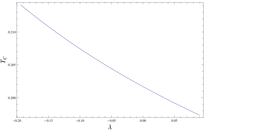
It is clear that is zero at and condensation occurs for . For positive Gauss-Bonnet coupling constant, it is true that the critical temperature decreases as becomes more positive, which means that condensation become harder to form for higher curvature corrections[31]. Considering that the Gauss-Bonnet constant is also allowed to be negative from causality, in Fig.2 we also plot the critical temperature for negative Gauss-Bonnet coupling constant. The condensates as functions of temperature by comparing the influences due to positive, zero and negative Gauss-Bonnet coupling constants are exhibited in Fig.3. We see that different from the positive Gauss-Bonnet coupling constant, the allowed negative coupling can enhance the condensation and make the superconducting phase easier to form.

3.2 Strong magnetic field limit
When the magnetic field is strong enough, we have to consider the spatially dependent solutions. It is consistent to take the ansatz
| (3.50) |
The main equation now governing the scalar field is
| (3.51) |
where . We can separate
| (3.52) |
where satisfies the equation for a two dimensional harmonic oscillator with frequency determined by
| (3.53) |
The solution of (3.53) is the Hermite function
| (3.54) |
where denotes the separation constant. We will choose the lowest mode in the following of our computation. After the separation of variables, we obtain the equation of motion for ,
| (3.55) |
The regularity at the horizon gives
| (3.56) |
Near the AdS boundary, we have
| (3.57) |
We will use the notation in the following computation. By expanding in a Taylor series near the horizon, we have
| (3.58) |
Near , (3.55) gives
| (3.59) | |||||
where . The approximate solution of near the horizon can be given by
| (3.60) | |||||
Matching (3.57) and (3.60) at the intermediate point , we obtain
| (3.61) | |||||
| (3.62) | |||||
Using Eqs.(3.61) and (3.62), we can eliminate and get
| (3.63) | |||||
By using and (3.41), we find the expression for the upper critical magnetic field , which turns out to be very long and involving. In order to have a simple formula, let us first fix the parameters as , , , and .
| (3.64) | |||||
By further using equation (3.49), we finally obtain
| (3.65) | |||||
where .
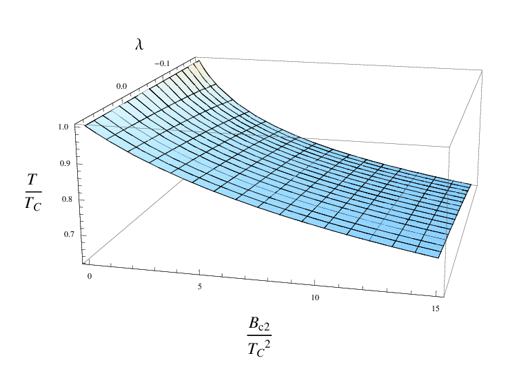
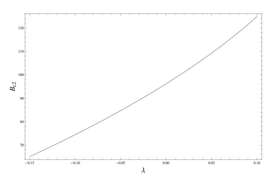

The expression for the upper critical magnetic field here is different from that in four dimensional holographic superconductors. One may find that as , the critical magnetic field diverges, but it works well for . This is true for all dimensional cases. There are several parameters in the above equation, which relate to the critical magnetic field in the presence of the Gauss-Bonnet coupling. Fixing the Gauss-Bonnet coupling constant, we can see from Fig.4 that the critical temperature decreases rapidly as the increase of the external magnetic field. The decrease is even faster for negative Gauss-Bonnet coupling, which shows that the magnetic field is expelled strongly on the condensate for the negative Gauss-Bonnet coupling situation. Fig.2 and Fig.4 also exhibit that when the magnetic field is not big enough, the influence given by the higher curvature on the condensation keeps the same as that for neglecting magnetic field: a more negative leads to the higher critical temperature while the bigger positive Gauss-Bonnet coupling results in the smaller critical temperature. Fig.5 exhibits that for fixed temperature , a more negative leads to the lower critical magnetic field while the bigger positive Gauss-Bonnet coupling results in the bigger critical magnetic field. Fig.6 shows us that higher temperature leads to lower critical magnetic field .
4 Conclusions and discussions
In this work we have investigated the holographic superconductors immersed in an external magnetic field by using the analytical method developed in [30, 31]. We have obtained the spatially dependent condensate solutions in the presence of the magnetism. We have found analytically that the upper critical magnetic field satisfies the relation , which is in agreement with that given in the Ginzburg-Landau theory. Further we found from the analytic approach that when the external magnetic field grows, the condensation will be harder to form, which indicates that the magnetic field expels the condensate as reported in [8, 12].
We have further extended our investigation to the D-dimensional Gauss-Bonnet AdS black holes and examined the influence given by the Gauss-Bonnet coupling on the condensation. In the presence of the magnetism we observed that the influence due to the positive Gauss-Bonnet coupling keeps the same which will hinder the condensation to form. Considering that the Gauss-Bonnet coupling constant can also be negative without violating the causality on the boundary theory, we have also examined the negative Gauss-Bonnet coupling effect on the condensation. We found that different from the positive coupling, the negative Gauss-Bonnet coupling can enhance the condensation when the external magnetic field is not strong enough. At the first glance the effect of the negative Gauss-Bonnet coupling violates the Mermin-Wagner theorem. However to examine whether or not the Mermin-Wagner theorem holds, one needs to concentrate on the -dimensional higher curvature gravity. Here we have studied the Gauss-Bonnet gravity in dimensions , which is non-trivial and ghost free. This may leave the space for the enhancement of the condensation due to the negative Gauss-Bonnet coupling. The similar relation between the upper critical magnetic field with the temperature to that in the Ginzburg-Landau theory has also been observed with the Gauss-Bonnet coupling.
Acknowledgments
We wish to thank R. K. Su, Q. Y. Pan, X. He, S. Y. Yin, Y. Peng and Y. Q. Liu for useful discussions. The work of BW was supported by the NSFC. The work of XHG and SFW were partially supported by NSFC under Grant Nos. 10947116 and 10905037, Shanghai Education Development Foundation, and Innovation Foundation of Shanghai University. XHG was also partly supported by Shanghai Rising-Star program and SRF for ROCS, SEM.
References
- [1] J. M. Maldacena, Adv. Theor. Math. Phys. 2 (1998) 231, [arXiv:hep-th/9711200].
- [2] S. S. Gubser, I.R. Klebanov and A.M. Polyakov, Phys. Lett. B428 (1998) 105, [arXiv:hep-th/9802109].
- [3] E. Witten, Adv. Theor. Math. Phys. 2 (1998) 253, [arXiv:hep-th/9802150].
- [4] S. S. Gubser, Class. Quant. Grav. 22, 5121 (2005).
- [5] S. S. Gubser, Phys. Rev. D 78, 065034 (2008).
- [6] S. A. Hartnoll, C. P. Herzog, and G. T. Horowitz, Phys. Rev. Lett. 101, 031601 (2008) [arXiv:0803.3295[hep-th]].
- [7] S. A. Hartnoll, C. P. Herzog, and G. T. Horowitz, arXiv:0810.1563.
- [8] T. Albash and C. V. Johnson, J. High Energy Phys. 09 121 (2008), [arXiv:0804.3466 [hep-th]]; T. Albash and C. V. Johnson, [arXiv:0906.0519[hep-th]].
- [9] A. Ammon, J. Erdmenger, M. Kaminski and P. Kerner, [arXiv:0810.2316[hep-th]]; [arXiv:0903.1864[hep-th]]
- [10] T. Albash and C. V. Johnson, arXiv:0906.1795 [hep-th].
- [11] M. Montull, A. Pomarol, and P. J. Silva, Phys. Rev. Lett 103 091601 (2009) [arXiv:0906.2396 [hep-th]].
- [12] K. Maeda, M. Natsuume and T. Okamura, Phys. Rev. D 81 026002 (2010) [arXiv:0910.4475 [hep-th]].
- [13] S. A. Hartnoll, C. P. Herzog, and G. T. Horowitz, J. High Energy Phys. 0812, 015 (2008).
- [14] G. T. Horowitz and M. M. Roberts, Phys. Rev. D 78, 126008 (2008).
- [15] E. Nakano and W. Y. Wen, Phys. Rev. D 78, 046004 (2008).
- [16] I. Amado, M. Kaminski, and K. Landsteiner, J. High Energy Phys. 0905, 021 (2009).
- [17] G. Koutsoumbas, E. Papantonopoulos and G. Siopsis, J. High Energy Phys. 0907, 026 (2009).
- [18] K. Maeda, M. Natsuume, and T. Okamura, Phys. Rev. D 78 106007 (2008); Phys. Rev. D 79, 126004 (2009).
- [19] J. Sonner, Phys. Rev. D 80, 084031 (2009).
- [20] H. Zeng, Z. Fan, Z. Ren, Phys. Rev. D 80, 066001 (2009); D. W. Pang, J. High Energy Phys. 10 031 (2009) [arXiv:0908.1272]; [arXiv:0911.2777]; J. High Energy Phys. 01 120 (2010)[arXiv:0912.2403].
- [21] S. J. Sin and I. Zahed, J. High Energy Phys. 12 015 (2009) [arXiv:0907.1434 [hep-th]].
- [22] R. G. Cai and H. Q. Zhang, Phys. Rev. D 81 066003 (2010) [arXiv: 0911.4867[hep-th]]; R. G. Cai, Z. Y. Nie and H. Q. Zhang, [arXiv: 1007.3321[hep-th]].
- [23] J. Jing, L. Wang, S. Chen, [arXiv:1001.2946]
- [24] S. J. Sin, S. Xu and Y. Zhou, [arXiv:0909.4857[hep-th]]; S. Pu, S. J. Sin, and Y. Zhou, [arXiv:0903.4185[hep-th]]
- [25] S. Chen, L. Wang, C. Ding and J. Jing, [arXiv:0912.2397]
- [26] G. Siopsis and J. Therrien, JHEP 05 (2010) 013 [arXiv:1003.4275].
- [27] S. A. Hartnoll, [arXiv: 0903.3246].
- [28] C. P. Herzog, J. Phys. A 42, (2009) 343001.
- [29] G. T. Horowitz, M. M. Roberts, JHEP 0911:015,2009.
- [30] R. Gregory, S. Kanno and J. Soda, J. High Energy Phys. 10, 010 (2009) [arXiv:0907.3203[hep-th]]
- [31] Q. Pan, Bin Wang, E. Papantonopoulos, J. Oliveria and A. B. Pavan,Phys.Rev.D 81, (2010) 106007 [arXiv:0912.2475[hep-th]]; Q. Pan and B. Wang, [arXiv:1005.4743 [hep-th]]; Y. Liu, Q. Pan, B. Wang and R. G. Cai, [arXiv:1007.2536 [hep-th]].
- [32] C. P. Poole, H. A. Farach and R. J. Creswick, “ Superconductivity”, Academic Press, Netherlands, (2007) .
- [33] D. M. Hofman, Nucl. Phys. B 823 174 (2009) [arXiv:0907.1625[hep-th]]
- [34] M. Brigante, H. Liu, R.C. Myers, S. Shenker and S. Yaida, Phys. Rev. Lett. 100 (2008) 191601, [arXiv:0802.3318[hep-th]].
- [35] X. H. Ge, Y. Matsuo, F.-W. Shu, S.-J. Sin and T. Tsukioka, J. High Energy Phys. 10, 009 (2008) [arXiv:0808.2354[hep-th]]
- [36] X. H. Ge and S.-J. Sin, J. High Energy Phys. 05, 051 (2009) [arXiv:0903.2527[hep-th]]
- [37] X. H. Ge, S. J. Sin, S. F. Wu and G. H. Yang, Phys. Rev. D 80, 104019 (2009) [arXiv:0905.2675[hep-th]]
- [38] A. Buchel and R. C. Myers, J. High Energy Phys. 08, 016 (2009) [arXiv:0906.2922[hep-th]]
- [39] R. G. Cai, Z. Y. Nie and Y. W. Sun, Phys. Rev. D 78, 126007 (2008) [arXiv:0811.1665 [hep-th]]; R. G. Cai, Z. Y. Nie, N. Ohta and Y.W. Sun, Phys. Rev. D 79, 066004 (2009) [arXiv:0901.1421 [hep-th]].
- [40] F. W. Shu, [arXiv:0910.0607[hep-th]]
- [41] J. de Boer, M. Kulaxizi and A. Parnachev, [arXiv:0910.5347[hep-th]]
- [42] A. Buchel, J. Escobedo, R. C. Myers, M. F. Paulos, A. Sinha, M. Smolkin, J. High Energy Phys. 03 111 (2010) [arXiv:0911.4257 [hep-th]]
- [43] X. O. Camanho and J. D. Edelstein, [arXiv:0911.3160[hep-th]]; [arXiv:0912.1944[hep-th]].
- [44] A. A. Abrikosov, L. P. Gorkov and I. E. Dzyaloshinski,“Methods of Quantum Field Theory in Statistical Physics.” Dover, New York (1963).
- [45] R. G. Cai, Phys. Rev. D 65 (2002) 084014, [arXiv:hep-th/0109133].
- [46] I. P. Neupane, Phys. Rev. D67 (2003) 061501, [arXiv:hep-th/0212092]; Phys. Rev. D69 (2004) 084011, [arxiv:hep-th/0302132].