Flavor Superconductivity & Superfluidity
Abstract
In these lecture notes we derive a generic holographic string theory realization of a p-wave superconductor and superfluid. For this purpose we also review basic D-brane physics, gauge/gravity methods at finite temperature, key concepts of superconductivity and recent progress in distinct realizations of holographic superconductors and superfluids. Then we focus on a D3/D7-brane construction yielding a superconducting or superfluid vector-condensate. The corresponding gauge theory is 3+1-dimensional supersymmetric Yang-Mills theory with color and flavor symmetry. It shows a second order phase transition to a phase in which a subgroup of the symmetry is spontaneously broken and typical superconductivity signatures emerge, such as a conductivity (pseudo-)gap and the Meissner-Ochsenfeld effect. Condensates of this nature are comparable to those recently found experimentally in p-wave superconductors such as a ruthenate compound. A string picture of the pairing mechanism and condensation is given using the exact knowledge of the corresponding field theory degrees of freedom.
Contents
1 Introduction
In these lecture notes11 1 These lecture notes are based on joint research work with Martin Ammon, Johanna Erdmenger, Patrick Kerner and Felix Rust. we generically construct a holographic p-wave superconductor. This introductory section serves to explain why this particular setup is of interest both from a string-theoretical as well as from a condensed matter physics point of view. In order to guide the unexperienced reader in section 2 we will describe the basic concepts in words and motivate the project. Detailing this overview we build the full holographic setup from scratch in a self-contained manner in section 3. Section 4 briefly introduces common holographic methods and then summarizes the major results known for the thermodynamics and the spectrum of D-brane systems. With these outcomes in the back of our minds we will understand how our system develops a new ground state and why it can be interpreted as a meson superfluid or superconductor. We compute and discuss thermodynamic observables, conductivities and the spectrum of our holographic superconductor in section 5. Finally, we put together all of our findings in order to draw a string theory picture for the pairing mechanism in our p-wave superconductor. These notes are self-contained and widely complementary to the notes focusing on holographic s-wave superconductors [1, 2, 3].
1.1 String motivation
The setup of intersecting D-branes and especially the particular D3-D7 construction presented here is interesting because of its diverse applications. It has been successfully used to model strongly coupled particle physics phenomena such as a deconfinement, or rather meson melting phase transition for fundamental matter and transport coefficients in the quark gluon plasma experimentally created at the RHIC collider in Brookhaven (see [4] for an introductory review and further references). On the other hand it has recently been used to model strongly correlated electron systems as they appear in superfluids and superconductors in the realm of condensed matter physics [5, 6]. All these applications are also crucial checks of the basic principles and methods coming from the conjectured gauge/gravity correspondence. Receiving physically meaningful outcomes when applying these holographic methods to various systems accessible by experiment, strengthens our confidence in the gauge/gravity conjecture.
From the string-theoretic point of view this particular setup is interesting because of its simplicity, uniqueness (explained below) and the naturalness with which the symmetry is broken spontaneously here. The flavor22 2 The term ”flavor” superconductor stems from earlier applications of this setup to model strongly correlated high energy systems such as the quark gluon plasma. In the present case the name is not important and possibly misguiding, since it is really only essential that the system has a non-Abelian symmetry. superfluid/superconductor33 3 We are using the terms superfluid and superconductor interchangably here. For the considered phenomena this distinction does not make any difference. Some details to this distinction are given in section 2.1. examined here was the first generic top-down string theory realization of a superfluid/superconducting phase. In contrast to this the pioneering papers on holographic superconductors [7, 8, 9] had exclusively treated gravity toy models which were not directly obtained from string theory, i. e. bottom-up models. Therefore the gauge/gravity correspondence could not be used to identify the exact gauge theory dual. This fact obstructed the interpretation of the outcomes. Furthermore these toy models had few restrictions on their parameters such that in principle a large parameter space needed to be scanned, see e. g. [10]. Our string-derived flavor superfluid/superconductor overcomes those two problems: First the field theory degrees of freedom are exactly known since it is simply supersymmetric Yang-Mills theory with an flavor-symmetry. Second, the values of parameters, such as for example the dimension of the condensing operator, in our setup are severly restricted by their string theoretic derivation. In this sense this setup is ”unique” compared to the big parameter space to be scanned in bottom-up toy models. Later, other top-down string realizations have been suggested and for example involve a consistent truncation of type IIB supergravity with a chemical potential for the R-charge [11], and domain-wall solutions interpolating between AdS solutions with distinct radii which may be lifted to IIB supergravity or eleven-dimensional supergravity [12].
1.2 Condensed matter motivation
From a condensed-matter physics point of view our flavor superconductor is highly interesting because it reproduces features which have been measured in experiments with unconventional superconductors, such as p-wave superconductivity, a system of strongly-correlated particles, a pseudo-gap in the frequency-dependent conductivity (found in high temperature d-wave superconductors). Most of these phenomena lack a widely-accepted microscopic explanation by conventional approaches, so there is the hope that gauge/gravity can shed some light on the nature of these systems. These systems usually contain strongly correlated electrons, so the dual weak gravity description is in principle accessible. Our system has a vector operator which condenses upon breaking a residual Abelian flavor symmetry spontaneously. This gives the vector order parameter as described below. So there is a preferred spatial direction in the superfluid/superconducting condensate. This is exactly the situation recently found experimentally in the p-wave (explained below in section 2.1) superconductor [13]. These materials are investigated with great excitement in the condensed-matter community because they are hoped to be usable for quantum computing [14]. The reason is that the p-wave structure implies the presence of non-Abelian quasi-particles in the ruthenate compound. These non-Abelian quasi-particles can be used as the states to be manipulated in a topological quantum computer. The biggest practical obstacle for quantum computation are the errors which may occur during a calculation due to materials being not ideal. Topological quantum computers minimize this source of error because they carry out operations by braiding the non-Abelian quasi-particles in a Hilbert-subspace containing degenerate ground states. Due to an energy gap between this subspace and the rest of the Hilbert space it virtually decouples from all local perturbations [15]. Another confirmed and well-studied condensed-matter example for an emerging p-wave structure is superfluid 3He-A [16].
2 Superconductivity & Holography
This section is a primer on the subject of spontaneous symmetry breaking, superconductivity and superfluidity in the holographic context of the gauge/gravity correspondence. Little formalism is used, while we introduce all the necessary concepts.
2.1 Basics of superconductivity & our field theory idea
Let us review the essential concepts of superconductivity and understand how to build a p-wave superconductor. We are going to need this knowledge in order to appreciate the fact that our holographic setup reproduces this behavior in great detail.
| Orbital angular momentum | Name | Parity of spatial part | Spin state |
| \svhline 0 | s-wave | even | singlet |
| 1 | p-wave | odd | triplet |
| 2 | d-wave | even | singlet |
Superconductor basics & the p-wave Superconductivity is the phenomenon associated with infinite dc conductvity in materials at low temperatures. It is caused by the formation of a charged condensate in which directed currents do not experience resistivity. A defining criterion for superconductivity is the Meissner-Ochsenfeld effect described below. In conventional superconductors the superconducting condensate consists of electron pairs called Cooper pairs. So there are two simultaneous steps: the fermionic electrons have to pair up to form bosonic Cooper pairs, and these pairs do condense. This condensation happens in a second order phase transition (at vanishing magnetic field) when the temperature is lowered through its critical value . Due to the requirement for the fermionic state to be antisymmetric there are only certain symmetry combinations allowed for the two electron state describing a Cooper pair. As seen from table 1 the name ”p-wave” superconductor refers to those pairs in which the relative orbital angular momentum between the two electrons is , the spatial part of the parity is odd and the spin state is a triplet.
The mechanism pairing electrons in conventional superconductors is well described by a mean field theory approach and the microscopic BCS-theory. Recall that condensed matter systems are conveniently described in terms of lattices with many (about ) sites. Then conventional BCS-theory tells us that the lattice is slightly deformed by the presence of an electron. This deformation can be described by a quasi-particle excitation, a phonon. We can imagine the phonon to create a small potential well near the electron in which another electron can be caught. So lattice vibrations (phonons) mediate a weakly attractive interaction between the electrons which then form pairs. Conventional BCS-theory with phonons is only valid at low temperatures because around the phononic lattice vibrations caused by the temperature already destroy the weakly attractive interaction between the electrons. Note that BCS-theory itself does not depend on the origin of the attractive interaction.
A superconductor is simply a charged superfluid. The crucial defining property for any kind of superconductivity or superfluidity is that a symmetry is spontaneously broken. In superfluids this symmetry is global while in superconductors it is local, i. e. a gauge symmetry. Therefore in superconductors there are a few additional effects related to the gauge symmetry and the corresponding gauge field. But besides that those two phenomena are very similar. Especially in both cases there is a Goldstone boson created for each spontaneously broken symmetry of the describing field theory. For a broken global symmetry this Goldstone boson survives and is visible in the spectrum as a hydrodynamic mode [17]. For a broken local symmetry however the Goldstone boson is eaten by the gauge field which couples to the charge belonging to the broken symmetry. In superconductors this causes the gauge boson, i. e. the photon for the broken electromagnetic to become massive. Since these heavy photons can travel only an exponentially small distance, the electromagnetic interaction becomes short-ranged. Therefore magnetic fields, which can be thought of as consisting of photons, can only penetrate the system up to a certain distance, the penetration depth. This is called Meissner-Ochsenfeld effect and it is a defining criterion for superconductivity. In the Anderson-Higgs mechanism particles acquire a mass by the same mechanism. Thus it is sometimes described as the superfluidity of the vacuum. See [18] for a more precise review.
There is a class of experimentally well-studied but theoretically less understood unconventional superconductors, such as copper or ruthenate compounds. Some of these materials show superconducting phases at high temperatures44 4 These high temperature superconductors in general realize a d-wave structure. However, belongs to a distinct class of unconventional superconductors and is p-wave superconducting at low temperatures around . The pairing mechansim is not microscopically understood. The simplified argument is that the phonon-interaction of conventional Cooper pairing is isotropic, thus not providing an anisotropic p-wave structure. up to . The conventional BCS-theory does not apply to such high temperatures as mentioned above. So the biggest mystery remains to understand the pairing mechanism of electrons in these high temperature superconductors. Pairing and condensation need not occur at the same temperature here. Most important for the application of gauge/gravity duality: In these unconventional superconductors the coupling strength of the electrons to each other is strong. Thus these are experimentally accessible systems governed by strongly coupled field theory.
Another clear signature for superconductivity is of course an infinite dc conductivity. Together with that there is a conductivity gap in the frequency-dependent conductivity. This is caused by the fact that the conductivity at small frequencies or energies vanishes until there is enough energy to break up one Cooper pair. From that energy on the material is a normal conductor with individual electrons being the charge carriers. In unconventional superconductors there is a surprising phenomenon called pseudo-gap. This means that the experiments carried out in unconventional superconductors show a gap in the conductivity even at and above the transition temperature where the superconducting condensate forms. Inside this pseudo-gap the conductivity does not drop to zero but to a small finite value.
How to build a field theory with p-wave superconductivity
[scale=.65]./phasediagram1BW.eps
As stressed above the crucial thing to do in order to get a superconductor or superfluid is to spontaneously break a symmetry. We are going to accomplish this by allowing our system to develop a charged condensate.
Let us assume a particle physics point of view for a while. In these notes we will focus on a 3+1 – dimensional supersymmetric Yang-Mills theory at temperature , consisting of a gauge multiplet as well as massive supersymmetric hypermultiplets The hypermultiplets give rise to the flavor degrees transforming in the fundamental representation of the gauge group. The action is written down explicitly for instance in [19]. In particular, we work in the large limit with at strong coupling, i. e. with where is the ’t Hooft coupling constant. In the following we will consider only two flavors, i. e. The flavor degrees of freedom are called and . If the masses of the two flavor degrees are degenerate, the theory has a global flavor symmetry, whose overall subgroup can be identified with the baryon number.
In the following we will consider the theory at finite isospin chemical potential , which is introduced as the source of the operator
| (1) |
where is the charge density of the isospin fields, and . are the Pauli matrices. A non-zero vev introduces an isospin density as discussed in [20]. The isospin chemical potential explicitly breaks the flavor symmetry down to , where is generated by the unbroken generator of the . Under the symmetry the fields with index and have positive and negative charge, respectively.
However, the theory is unstable at large isospin chemical potential [20]. The new phase is sketched in figure 1. We show in this lecture (see also [5]), that the new phase is stabilized by a non–vanishing vacuum expectation value of the current component
| (2) |
This current component breaks both the rotational symmetry as well as the remaining Abelian flavor symmetry spontaneously. The rotational is broken down to , which is generated by rotations around the axis. Due to the non–vanishing vev for flavor charged vector mesons condense and form a superfluid. Let us emphasize that we do not describe a color superconductor on the field theory side, since the condensate is a gauge singlet. Figure 1 shows a ”not accessable” parameter region in which we get divergent quantities. This is due to the fact that at such large charge densities we would need to take in account the backreaction of the D-branes on the AdS geometry.
In a condensed matter context our model can be considered as a holographic p–wave superconductor in the following way. The global in our model is the analog of the local symmetry of electromagnetic interactions. So far in all holographic models of superconductors the breaking of a global symmetry on the field theory side is considered. In our model, the current corresponds to the electric current The condensate breaks the spontaneously. Therefore it can be viewed as the superconducting condensate, which is analogous to the Cooper pairs. Since the condensate transforms as a vector under spatial rotations, it is a p--wave superconductor. -- Strictly speaking, for a superconductor interpretation it would be necessary to charge the superfluid, i. e. gauge the global symmetry which is broken spontaneously in our model. A spontaneously broken global symmetry corresponds to a superfluid. However, as we mentioned before many features of superconductivity do not depend on whether the is gauged. One exception to this is the Meissner–Ochsenfeld effect. To generate the currents expelling the magnetic field, the symmetry has to be gauged. This matter is discussed further below in section 5.4 where we will be able to see the onset of the Meissner–Ochsenfeld effect within our holographic setup.
2.2 Holographic realization
Holographic superconductors have first been studied in [21, 22, 7, 8]. The initial idea presented in [21] was that the Abelian Higgs model coupled to gravity with a negative cosmological constant provides a charged scalar condensate near but outside a charged black hole horizon. The charged condensate spontaneously breaks the Abelian gauge symmetry of the theory. Later studies revealed that this breaking also occurs in setups with neutral black holes but with a negative mass for the charged scalar [7]. The basic idea for a holographic p-wave superconductor has been outlined in [8]. Let us review the basic ideas.
Holographic superconductor basics In order to spontaneously break a symmetry we need a gravity theory with a gauge symmetry. Note that this is not the usual gauge symmetry of the correspondence where , but an additional one with a finite rank, for example an Abelian . Furthermore we need a black hole background in order to introduce finite temperature in the dual field theory, see [4] for details. Most importantly we need a charged condensate hovering in the bulk over the horizon. To be more precise, we need a bulk field charged under the gauge symmetry which is to be broken. has to have the typical expansion near the AdS boundary, but with . Why do we require this particular structure? Recall that in the gauge/gravity correspondence the normalizable mode is identified with the field theory expectation value of the operator dual to the gravity field . This is our condensate in the field theory, which we want to be non-zero. The normalizable mode on the other hand is dual to a source in the field theory. Therefore we want it to vanish since it would break the symmetry explicitly. The role of the field providing the condensate could be played for example by a charged scalar or by one component of a gauge field. These concepts are illustrated in the following example.
\runinheadExample: Consider the bottom-up toy model p-wave superconductor introduced in [8]. There we have an Einstein Yang-Mills theory with a negative cosmological constant
| (3) |
with being the field strength of an gauge field . This in this case is the gauge group that we want to break. Actually we break only a subgroup of it. But let us not worry about the details now. Only note that this theory is placed in an AdS4 charged black hole background. Our gauge field now plays the role of the field providing the condensate. The operator dual to the gauge field is the electromagnetic current . The boundary behavior of the gravity field’s components according to the equations of motion derived from equation (3) is given by
| (4) |
with the radial AdS coordinate . In principle we could allow more non-vanishing components but this combination turns out to be both sufficient and consistent. As usual in thermal AdS/CFT the temporal component introduces a chemical potential in the dual field theory. This chemical potential sources the corresponding operator which is simply the charge density of the charge in the field theory at the boundary. This explicitly breaks . However the spatial component spontaneously breaks the remaining with the condensate .
How to build a gravity dual to p-wave superconductivity As mentioned several times before, we need a vector condensate for our p-wave superconductor. Conveniently the previous example already showed us what the structure for the dual gravity theory has to be in order to realize a vector condensate. Unfortunately that example has not been derived from string theory. Probably the most difficult task in building a holographic superconductor is finding a gravity setup with all the neccessary features, which is actually stable and thermodynamically favored. We are going to see that the system of intersecting D3 and D7 branes provides exactly such a stable configuration. Since we are going to review Dp/Dq- brane systems below, let us here spot only those features which are of importance to superconductivity. The ”flavor” gauge group which we are going to break (partly spontaneously) is created by using two coincident D7 branes. By introducing a gauge field living on these D7-branes and giving its temporal component a non-trivial profile in one of the flavor directions, we introduce a chemical potential in the dual field theory. This is completely analogous to introducing the non-trivial in the previous example. All this is going to take place in the background of a stack of black D3-branes. They introduce the temperature into the dual field theory. Finally, the gravity field which will break the residual flavor symmetry is going to be a spatial component of the gauge field just as in the previous example. Our analysis of the thermodynamic potentials is going to show that this phase is thermodynamically preferred over the phase without the symmetry-breaking condensate. Furthermore it is stable against all obvious gauge field fluctuations.
3 Holographic setup
In this section we carry out exactly the D3-D7 brane construction outlined in section 2.2. The result will be a gravity setup being holographically dual to a p-wave superfluid/superconductor. But let us first review how to add flavor to the gauge/gravity correspondence.
3.1 Flavor from intersecting branes
Let us imagine for this subsection that we want to use gauge/gravity in order to model QCD or the quark gluon plasma state of matter produced at the RHIC Brookhaven heavy-ion collider. The original AdS/CFT conjecture does not include matter in the fundamental representation of the gauge group but only adjoint matter. In order to come closer to a QCD-like behavior one can therefore investigate how to incorporate quarks and their bound states in this section. We focus on the main results of [23] and [24], however for a concise review the reader is referred to [19].
Since AdS/CFT has been discovered a lot of modifications of the original conjecture have been proposed and analyzed. This is always achieved by modifying the gravity theory in an appropriate way. For example the metric on which the gravity theory is defined may be changed to produce chiral symmetry breaking in the dual gauge theory [25, 26]. Other modifications put the gauge theory at finite temperature and produce confinement [27]. Besides the introduction of finite temperature the inclusion of fundamental matter, i.e. quarks, is the most relevant extension for us since we are aiming at a qualitative description of strongly coupled QCD effects at finite temperature. These effects are similar to the ones observed at the RHIC heavy ion collider.
Adding flavor to AdS/CFT The change we have to make on the gravity side in order to produce fundamental matter on the gauge theory side is the introduction of a small number of D7-branes. These are also called probe branes since their backreaction on the geometry originally produced by the stack of D3-branes is neglected. Strings within this D3/D7-setup now have the choice of starting (ending) on the D3- or alternatively on the D7-brane. Note that the two types of branes share the four Minkowski directions in which also the dual gauge theory will extend on the boundary of AdS as visualized in figure 2.
| 0 | 1 | 2 | 3 | 4 | 5 | 6 | 7 | 8 | 9 | |
|---|---|---|---|---|---|---|---|---|---|---|
| D3 | x | x | x | x | ||||||
| D7 | x | x | x | x | x | x | x | x |
The configuration of one string ending on coincident D3-branes produces an gauge symmetry of rotations in color space. Similarly the D7-branes generate a flavor gauge symmetry. We will call the strings starting on the stack of D-branes and ending on the stack of D-branes strings. The original strings are unchanged while the - or equivalently strings are interpreted as quarks on the gauge theory side of the correspondence. This can be understood by looking at the strings again. They come in the adjoint representation of the gauge group which can be interpreted as the decomposition of a bifundamental representation . So the two string ends on the D3-brane are interpreted as one giving the fundamental, the other giving the anti-fundamental representation in the gauge theory. In contrast to this the string has only one end on the D3-brane stack corresponding to a single fundamental representation which we interpret as a single quark in the gauge theory.
We can also give mass to these quarks by separating the stack of D3-branes from the D7-branes in a direction orthogonal to both branes. Now strings are forced to have a finite length which is the minimum distance between the two brane stacks. On the other hand a string is an object with tension and if it assumes a minimum length, it needs to have a minimum energy being the product of its length and tension. The dual gauge theory object is the quark and it now also has a minimum energy which we interpret as its mass .
The strings decouple from the rest of the theory since their effective coupling is suppressed by . In the dual gauge theory this limit corresponds to neglecting quark loops which is often called the quenched approximation. Nevertheless, they are important for the description of mesons as we will see below.
Let us be a bit more precise about the fundamental matter introduced by strings. The gauge theory introduced by these strings (in addition to the original setup) gives a supersymmetric gauge theory containing fundamental hypermultiplets.
D7 embeddings & meson excitations Mesons correspond to fluctuations of the D7-branes55 5 To be precise the fluctuations correspond to the mesons with spins 0, 1/2 and 1 [24, 28]. embedded in the -background generated by the D3-branes. From the string-point of view these fluctuations are fluctuations of the hypersurface on which the strings can end, hence these are small oscillations of the string ends. The strings again lie in the adjoint representation of the flavor gauge group for the same reason which we employed above to argue that strings are in the adjoint of the (color) gauge group. Mesons are the natural objects in the adjoint flavor representation. Vector mesons correspond to fluctuations of the gauge field on the D7-branes.
Before we can examine mesons as D7-fluctuations we need to find out how the D7-branes are embedded into the 10-dimensional geometry without any fluctuations. Such a stable configuration needs to minimize the effective action. The effective action to consider is the world volume action of the D7-branes which is composed of a Dirac-Born-Infeld and a topological Chern-Simons part
| (5) | |||||
| (6) |
The preferred coordinates to examine the fluctuations of the D7 are obtained from the standard AdS coordinates
| (7) |
with the AdS radius and the dimensionful radial AdS coordinate . \runinheadExercise Show that the standard AdS metric (7) transforms to
| (8) |
under the transformation , where is a four vector in Minkowski directions and is the AdS radius. The coordinate is the radial AdS coordinate while is the radial coordinate on the coincident D7-branes.
Let us follow [24]: For a static D7 embedding with vanishing field strength on the D7 world volume the equations of motion are
| (9) |
where denotes that these are two equations for the two possible directions of fluctuation. Since (9) is the equation of motion of a supergravity field in the bulk, the solution near the AdS boundary takes the standard form with a non-normalizable and a normalizable mode, or source and expectation value respectively
| (10) |
with being the quark mass acting as a source and being the expectation value of the operator which is dual to the field . While can be related to the scaled quark condensate .
If we now separate the D7-branes from the stack of D3-branes the quarks become massive and the radius of the on which the D7 is wrapped becomes a function of the radial AdS coordinate . The separation of stacks by a distance modifies the metric induced on the D7 such that it contains the term . This expression vanishes at a radius such that the shrinks to zero size at a finite AdS radius.
Fluctuations about these and embeddings give scalar and pseudoscalar mesons. We take
| (11) |
After plugging these into the effective action (5) and expanding to quadratic order in fluctuations we can derive the equations of motion for and . As an example we consider scalar fluctuations using an Ansatz
| (12) |
where are the scalar spherical harmonics on the , solves the radial part of the equation and the exponential represents propagating waves with real momentum . We additionally have to assume that the mass-shell condition
| (13) |
is valid. Solving the radial part of the equation we get the hypergeometric function and the parameter
| (14) |
summarizes a factor appearing in the equation of motion. In general this hypergeometric function may diverge if we take . But since this is not compatible with our linearization of the equation of motion in small fluctuations, we further demand normalizability of the solution. This restricts the sum of parameters appearing in the hypergeometric function to take the integer values
| (15) |
With this quantization condition we determine the scalar meson mass spectrum to be
| (16) |
where is the radial excitation number found for the hypergeometric function. Similarly we can determine pseudoscalar masses and find the same formula 16. For vector meson masses we need to consider fluctuations of the gauge field appearing in the field strength in equation (5). The formula for vector mesons (corresponding to e.g. the -meson of QCD) is
| (17) |
Note that the scalar, pseudoscalar and vector mesons computed within this framework show identical mass spectra. Further fluctuations corresponding to other mesonic excitations can be found in [24, 28].
Brane embeddings at finite temperature In order to get a finite temperature in the dual field theory, the gravity theory needs to be put into a black hole or black brane background geometry. It was found in [26, 29, 30] that at finite temperature our probe flavor branes can be embedded in two distinct ways. There are high temperature configurations called black hole embeddings in which part of the brane falls into the black hole horizon. On the other hand there are low-temperature configurations called Minkowski embeddings in which the brane stays outside the black hole horizon. These two configurations are separated by a geometric transition, i. e. the configuration in which the brane just barely touches the black hole horizon. This geometric transition corresponds to the meson melting transition for the fundamental matter of the dual field theory. Note that the adjoint matter of this field theory is always deconfined in this setup.
At finite charge density however there is only one kind of embedding and that is the black hole embedding. The heuristic argument is that introducing a finite charge on the brane there have to be field lines for the associated field strength. These lines have to end somewhere. Our setup has rotational symmetry in the spatial directions. Imagine the radial AdS coordinate and field lines running along it. If they are supposed to end somewhere, there has to be a horizon. Otherwise they would all meet in the origin at . Note that field lines ending at the horizon means, that we can interpret the horizon as being charged. In these lecture notes we will exclusively deal with non-vanishing density and thus only encounter black hole embeddings.
3.2 Background and brane configuration
We aim to have a field theory dual at finite temperature. This is holographically accomplished by placing the gravity theory in a black hole or black brane background. Here the black hole’s Hawking temperature can be identified with the field theory temperature. We consider asymptotically space-time. The geometry is holographically dual to the Super Yang-Mills theory with gauge group . The dual description of a finite temperature field theory is an AdS black hole. We use the coordinates of [31] to write the AdS black hole background in Minkowski signature as
| (18) |
with the metric of the unit 5-sphere and
| (19) |
where is the AdS radius, with . \runinheadExercise: Show that the metric (18) can be obtained from the standard finite temperature AdS metric
| (20) |
by the transformation , with being the original radial AdS coordinate and the location of the black hole horizon.
\runinheadExercise: The temperature of the black hole given by (18) may be determined by demanding regularity of the Euclidean section. Show that it is given by
| (21) |
In the following we may use the dimensionless coordinate , which covers the range from the event horizon at to the boundary of the AdS space at .
[width=0.6]./tableCoords.eps
To include fundamental matter, we embed coinciding D-branes into the ten-dimensional space-time as illustrated in figure 2. These D-branes host flavor gauge fields with gauge group . To write down the DBI action for the D-branes, we introduce spherical coordinates in the 4567-directions and polar coordinates in the 89-directions [31]. The angle between these two spaces is denoted by (). The six-dimensional space in the -directions is given by
| (22) |
where , and . D3- and D7-branes always share the four Minkowski directions and may be separated in the -directions which are orthogonal to both brane types. That separation is dual to the mass of the fundamental flavor fields in the dual gauge theory, i. e. the quarks.
Due to the rotational symmetry in the 4567 directions, the embedding of the D-branes only depends on the radial coordinate . Defining , we parametrize the embedding by and choose using the symmetry in the 89-direction. The induced metric on the D-brane probes is then
| (23) |
The square root of the determinant of is given by
| (24) |
where is the determinant of the 3-sphere metric.
As in [20] we introduce a isospin chemical potential by a non-vanishing time component of the non-Abelian background field on the D-brane. The generators of the gauge group are given by the Pauli matrices . Due to the gauge symmetry, we may rotate the flavor coordinates until the chemical potential lies in the third flavor direction,
| (25) |
This non-zero gauge field breaks the gauge symmetry down to generated by the third Pauli matrix . The spacetime symmetry on the boundary is still . Notice that the Lorentz group is already broken down to by the finite temperature. In addition, we consider a further non-vanishing background gauge field which stabilizes the system for large chemical potentials. Due to the symmetry of our setup we may choose to be non-zero. To obtain an isotropic configuration in the field theory, this new gauge field only depends on . Due to this two non-vanishing gauge fields, the field strength tensor on the branes has the following non-zero components, {svgraybox}
| (26) | |||
| (27) | |||
| (28) |
The labels behind those equations refer to the sort of strings which generate the corresponding gauge fields. The field strength can be understood as an interaction term between 7–7 and 3–7 strings. We derive this interpretation in section 6.1.
3.3 DBI action and equations of motion
In this section we calculate the equations of motion which determine the profile of the D-brane probes and of the gauge fields on these branes. A discussion of the gauge field profiles, which we use to give a geometrical interpretation of the stabilization of the system and the pairing mechanism, may be found in section 6.1.
The DBI action determines the shape of the brane embeddings, i. e. the scalar fields , as well as the configuration of the gauge fields on these branes. We consider the case of coincident D-branes for which the non-Abelian DBI action reads [32]
| (29) |
with
| (30) |
and the pullback to the D-brane, where for a D-brane in dimensions we have , , , . In our case we set , , . As in [20] we can simplify this action significantly by using the spatial and gauge symmetries present in our setup. The action becomes
| (32) | |||||
where in the second line the determinant is calculated. Due to the symmetric trace, all commutators between the matrices vanish. It is known that the symmetrized trace prescription in the DBI action is only valid up to fourth order in [33, 34]. However the corrections to the higher order terms are suppressed by [35] (see also [36]). Here we use two different approaches to evaluate the non-Abelian DBI action (32). First, we modify the symmetrized trace prescription by omitting the commutators of the generators and then setting (see subsection 3.3 below). This prescription makes the calculation of the full DBI action feasible. This prescription is not verified in general but we obtain physically reasonable results as discussed in section 5.1 and 5.2. Second, we expand the non-Abelian DBI action to fourth order in the field strength (see subsection 3.3). Here it should be noted that in general the higher terms of this expansion need not be smaller than the leading ones. However, we again get physical results in our specific case which confirm this approach. We further motivate the validity of our two approaches below.
Adapted symmetrized trace prescription
Using the adapted symmetrized trace prescription defined above, the action becomes
| (33) | |||||
with
| (34) | |||||
where the dimensionless quantities and are used. To obtain first order equations of motion for the gauge fields which are easier to solve numerically, we perform a Legendre transformation. Similarly to [31, 20] we calculate the electric displacement and the magnetizing field which are given by the conjugate momenta of the gauge fields and ,
| (35) |
In contrast to [31, 37, 38, 20], the conjugate momenta are not constant any more but depend on the radial coordinate due to the non-Abelian term in the DBI action. For the dimensionless momenta and defined as
| (36) |
we get
| (37) |
Finally, the Legendre-transformed action is given by
| (38) | |||||
| (39) |
with
| (40) | |||||
Then the first order equations of motion for the gauge fields and their conjugate momenta are
| (41) | |||||
| (42) | |||||
| (43) | |||||
| (44) |
with
| (45) |
For the embedding function we get the second order equation of motion
| (46) | |||||
We solve the equations numerically and determine the solution by integrating the equations of motion from the horizon at to the boundary at . The initial conditions may be determined by the asymptotic expansion of the gravity fields near the horizon
| (47) | |||||
| (48) | |||||
| (49) | |||||
| (50) | |||||
| (51) |
where the terms in the expansions are arranged according to their order in . For the numerical calculation we consider the terms up to sixth order in . The three independent parameter , and may be determined by field theory quantities defined via the asymptotic expansion of the gravity fields near the boundary,
| (52) | |||||
| (53) | |||||
| (54) | |||||
| (55) | |||||
| (56) |
According to the AdS/CFT dictionary, is the isospin chemical potential. The parameters are related to the vev of the flavor currents by
| (57) |
and and to the bare quark mass and the quark condensate ,
| (58) |
respectively. There are two independent physical parameters, e. g. and , in the grand canonical ensemble. From the boundary asymptotics (52), we also obtain that there is no source term for the current . Therefore as a non-trivial result we find that the symmetry is always broken spontaneously. In contrast, in the related works on p-wave superconductors in dimensions [8, 39], the spontaneous breaking of the symmetry has to be put in by hand by setting the source term for the corresponding operator to zero. With the constraint and the two independent physical parameters, we may fix the three independent parameters of the near-horizon asymptotics and obtain a solution to the equations of motion.
Expansion of the DBI action
We now outline the second approach which we use. Expanding the action (32) to fourth order in the field strength yields
| (59) |
where consists of the terms with order in . To calculate the , we use the following results for the symmetrized traces
| (60) | |||||
| (61) |
where the indices are distinct. Notice that the symmetric trace of terms with unpaired matrices vanish, e. g. . The are given in the appendix of [6].
To perform the Legendre transformation of the above action, we determine the conjugate momenta as in (35). However, we cannot easily solve these equations for the derivative of the gauge fields since we obtain two coupled equations of third degree. Thus we directly calculate the equations of motion for the gauge fields on the D-branes. The equations are given in the appendix of [6].
To solve these equations, we use the same strategy as in the adapted symmetrized trace prescription discussed above. We integrate the equations of motion from the horizon at to the boundary at numerically. The initial conditions may be determined by the asymptotic behavior of the gravity fields near the horizon
| (62) | |||||
| (63) | |||||
| (64) |
For the numerical calculation we use the asymptotic expansion up to sixth order. As in the adapted symmetrized trace prescription, there are again three independent parameters . Since we have not performed a Legendre transformation, we trade the independent parameter in the asymptotics of the conjugate momenta in the symmetrized trace prescription with the independent parameter (cf. asymptotics in equation (47)). However, the three independent parameters may again be determined in field theory quantities which are defined by the asymptotics of the gravity fields near the boundary
| (65) | |||||
| (66) | |||||
| (67) |
The independent parameters are given by field theory quantities as presented in (57) and (58). Again we find that there is no source term for the current , which implies spontaneous symmetry breaking. Therefore the independent parameters in both prescriptions are the same and we can use the same strategy to solve the equations of motion as described below (58).
\runinheadExercise: In [40] only the leading order of the action (59) quadratic in field fluctuations was considered. For a specific chemical potential an analytic solution with non-zero and can be found. Show that the analytic solution found there (adapted to our AdS5 case)
| (68) |
indeed solves the equations of motion derived from the action expanded to quadratic order for the chemical potential . is a constant formed from the coupling constant and the vacuum expectation value of the dual current . Note: This exercise requires some work. See also [41] for an application of this solution.
4 D-brane thermodynamics & spectrum
In this section we briefly review the results obtained for the thermodynamics and the spectrum of our setup with a baryonic, and later an isospin chemical potential.
[width=0.6]./grandcanPhaseDiagBBW.eps
4.1 Baryon chemical potential
Figure 4 shows the phase diagram of the field theory dual to the gravity setup we have constructed in the previous section 3. In this field theory we have introduced a baryonic chemical potential which is shown on the vertical axis scaled by the quark mass defined by equation (58). It is introduced by a non trivial background gauge field solving the equation of motion derived from the DBI-action and asymptoting to the chemical potential near the boundary as . The horizontal axis shows the scaled temperature . Recall that is the asymptotic value of the D7-brane embedding near the AdS boundary. In other words it is the source term for a quark condensate, or the non-normalizable mode of the brane embedding function. Here however we use it merely as a temperature scale. The lines in the diagram in figure 4 are lines of equal baryon density . At low temperature and chemical potential there is a triangle-shaped phase of zero density. Its diagonal borderline to the white region with finite baryon density is the location of the so-called meson-melting transition. This is the transition where the fundamental matter melts, i. e. quark bound states, the mesons, acquire an increasing decay width becoming quasi-particles. In the grey phase we therefore have stable mesons with zero decay width. The deeper we go into the white phase away from the transition line, the mesons melt. We will also see this in the spectral functions computed below. As explained at the end of section 3.1 we are going to stay entirely in the white phase at finite temperature where the brane embeddings are of black hole type, which means that part of them falls into the black hole horizon (see section 3.1).
Correlator recipe
We need to examine fluctuations of the fields in our setup in order to determine its spectrum and stability. There might be a fluctuation which is tachyonic and therefore could destabilize the whole system. For this purpose we quickly review how to compute real-time correlation functions in gauge/gravity.
Let us work along the example of a gauge field fluctuation . This appears in the action, in our case the Dirac-Born-Infeld action, in the field strength . Note that a background gauge field would appear in this field strength too, as we will see in later sections. For simplicity we consider Abelian gauge field fluctuations without background , i. e. . The action then reads something like
| (69) |
with the being the pullback of the metric to the flavor brane. Expanding this action to quadratic order in fluctuations , we get the linearized equation of motion for example for the spatial fluctuation which in Fourier space looks like this
| (70) |
where is the dimensionless frequency of the fluctuation. Also for other fields we end up with a second order differential equation that we need to solve. Usually these equations have singular (at the horizon ) coefficients which need to be regularized by an appropriate ansatz. In order to find the most singular behavior solving this equation, we plug the ansatz into equation (70) and expand. The leading order is a quadratic equation which can be solved for giving or . Only one of those two solutions, describes a fluctuation falling into the horizon, the other one is outgoing. We discard the outgoing one because nothing is supposed to leave a classical black hole. is sometimes called the indicial exponent. Now we plug , with being a regular function of , into the equation of motion (70). Note that there might be logarithmic terms present as explained in general for example in [43] and discussed in detail in [4]. Picking the ingoing wave fixes one of the two boundary conditions. The other boundary condition may be fixed by choosing the normalization of , i. e. the value . All the higher depend recursively on and the indicial exponent . Now we solve the equation for analytically or numerically. The correlator is then obtained from the quadratic part of the on-shell action, which in our case has the structure , where is a function of depending on metric coefficients. The recipe developed in [44, 45] tells us to strip the boundary values off from the fields and identify what remains of the integrand with the Green function at the boundary
| (71) |
Now we only need to plug in our solutions . More details on the analytic and numerical procedures are explained in [4].
Spectral function & quasi-normal modes
The spectral function is obtained from the imaginary part of the Green function . It encodes the spectrum of our thermal field theory. In particular in figure 5 we are able to identify pretty stable quasi-particle excitations at a low finite temperature parametrize by and at finite baryon density . Lowering the temperature these quasiparticles approach the line spectrum (17) indicated here as dashed vertical lines. The reason is that at lower temperature our theory restores its original supersymmetry. This also tells us that the vector quasi-particles we see in the thermal spectral function are vector mesons. Our mesons melt in the finite temperature, finite density phase as mentioned above in the discussion of the phase diagram 4.
Quasi normal modes (QNM) The difference between the zero temperature line spectrum and the finite temperature spectrum of quasi-particle excitations lies in the nature of the corresponding eigenmodes. In the zero temperature case there is no black hole, thus no dissipation on the gravity side. The system has well-defined normal modes at real frequencies . At finite temperature however the (quasi) eigenfrequencies are complex owing to the dissipation into the field theory plasma or in the dual gravity picture: dissipation into the black hole. The modes traveling with these (quasi) eigenfrequencies are called quasi-normal modes (QNM). We can roughly think of quasi-normal modes as being those solutions to the gravity fluctuation equations which vanish at the AdS boundary. These QNMs have been found to be identical to the poles in the field theory Green function. Therefore the location of the QNMs is closely related to the location of the peaks in the spectral function. At least some of the quasi-normal modes create quasi-particle peaks in the spectral function. In the zero temperature limit we can think of those QNMs as approaching the real frequency axis and reaching it in the limit, becoming real-valued. The corresponding quasiparticles become stable which means line-shaped in the spectrum. A more complete picture of QNMs is given in [46]. Quasi normal modes of our particular D3/D7 system are discussed in [47, 48].
[width=0.6]./plot4BW.eps
4.2 Isospin chemical potential
[width=.63]./isospinSplittingBW.eps
We can equally well introduce a chemical potential with –let’s call it isospin– structure, represented by the Pauli matrices . Choosing the chemical potential to point along the third flavor direction this background boils down to having two copies of the Abelian background gauge field explored above in the following way
| (72) |
However we get some interesting new signatures through the structure. For example the spectrum shown in figure 6 shows a triplet splitting for our mesons. In particular we observe a splitting of the line expected at the lowest meson mass at (). The resonance is shifted to lower frequencies for and to higher ones for , while it remains in place for . The second meson resonance peak () shows a similar behavior. So the different flavor combinations propagate differently and have distinct quasi-particle resonances. This behavior is analogous to that of QCD’s meson which is vector meson and a triplet under the isospin of QCD. Thus we have modeled the melting process of vector mesons in a quark gluon plasma at finite isospin density.
4.3 Instabilities & the new phase
What does all this have to do with our condensed matter motivation? The crucial thing is that the isospin setup described above develops an instability at large enough isospin density. This means that the modes and develop quasi-normal modes (QNM) which have a positive imaginary part, i. e. which are enhanced instead of being damped. This suggests that exactly the mesons corresponding to the fluctuations condense. This instability comes about naturally if we think about the fact, that we are trying to push more and more charge density into a confined volume. In particular the 3–7 strings charging the D7-brane are located at the black hole horizon as motivated earlier in section 3.1. Our current setup does not allow the strings to move into the bulk because we are forcing all the background fields they would create there to be zero. Up to now we have required and for all other field components. But we are going to relax that restriction by allowing a non-trivial . We will see below that this is sufficient to stabilize the theory in a new phase which we will prove to be superconducting/superfluid. This setup naturally produces a p-wave structure since we have seen above that the condensing vector mesons have a triplet structure. According to table 1 this implies a p-wave (at least to leading order).
5 Signatures of super-something
Finally we put together everything we have learned about D-branes, superconductors and holographic methods. We discuss the holographic results and interprete them in the condensed matter context. Section 5.1 starts with the thermodynamics and section 5.2 continues with the details of the fluctuation computation. The spectrum and conductivity is examined in section 5.3 and all the signatures will be pointing to the fact that we have indeed created a holographic p-wave superconductor/superfluid.
5.1 Thermodynamics of the broken phase

Figure 7 shows the background field configuration. The different curves correspond to the temperatures and . The plots are obtained at zero quark mass and by using the adapted symmetrized trace prescription. Similar plots may also be obtained at finite mass and by using the DBI action expanded to fourth order in . These plots show the same features: (top left) The gauge field increases monotonically towards the boundary. At the boundary, its value is given by the dimensionless chemical potential . (top right) The gauge field is zero for . For , its value is non-zero at the horizon and decreases monotonically towards the boundary where its value has to be zero. (bottom left) The conjugate momentum of the gauge field is constant for . For , its value increases monotonically towards the boundary. Its boundary value is given by the dimensionless density . (bottom right) The conjugate momentum of the gauge field is zero for . For , its value increases monotonically towards the boundary. Its boundary value is given by the dimensionless density .
All thermodynamic quantities are determined in terms of the relevant thermodynamic potential. We use the grand potential in the grandcanonical and the free energy in the canonical ensemble. Both stem from the D7-brane action. They are related through a Legendre transformation in the background gauge field on the gravity side. We obtain both potentials due to the gauge/gravity dictionary from the Euclideanized gravity on-shell action according to , with the partition function of the boundary field theory. So the for example .

Comparison of the grand potentials in figure 8 then shows that the new phase with a finite value for is thermodynamically preferred below a temperature and does not exist above. The transition seems numerically smooth, i. e. it is a continuous phase transition. In these respects both computation schemes, the symmetrized trace prescription as well as the DBI expansion to fourth order give the same qualitative behavior.
[width=0.6]./d13.eps
Figure 9 confirms this result and at least numerically determines the transition to be of second order. The order parameter vanishes with a critical exponent of to numerical accuracy. It has been explicitly verified that this condensation of vector particles occurs before, i. e. at higher temperature than the condensation of the scalars in our theory (see remarks in [6]). If this was QCD the scalar pions would condense before the vector mesons did. However, there might be other instabilities and also other symmetry breaking configurations may be possible.
[width=0.55]./ds.eps
Using some intuition to define the superconducting density , we find that it vanishes linearly at the critical temperature as shown in figure 10. {svgraybox} All these signatures are those of a superconducting/superfluid phase transition. The order parameter has vector structure by construction, which implies the p-wave.
[width=0.55]./Cv.eps
We can also compute the specific heat which the flavor branes contribute to the theory as . In figure 11 the higher curve corresponds to the normal phase with while the lower one corresponds to the superconducting phase with . Note that the total specific heat is always positive although the flavor brane contribution is negative. The divergences near in both phases can be attributed to the missing backreaction in our setup66 6 The backreaction of the gauge field on the geometry, i. e. on the Einstein equations for metric components has been considered in [49].. We read off from the numerical result that near the critical temperature, the dimensionless specific heat is constant in the superconducting phase. {svgraybox} This implies that the dimensionful specific heat is proportional to . This temperature dependence is characteristic for Bose liquids. There is also a finite jump in the specific heat at .
5.2 Fluctuations in the broken phase
Let us now investigate fluctuations of this system. We are going to see that the computation of the non-Abelian DBI-action is a very subtle issue. We argue for a novel prescription which actually gives reasonable results. The full gauge field on the branes consists of the field and fluctuations ,
| (73) |
where are the generators. The linearized equations of motion for the fluctuations are obtained by expanding the DBI action in to second order. We will analyze the fluctuations and , .
Including these fluctuations, the DBI action reads
| (74) |
with the non-Abelian field strength tensor
| (75) |
where the background is collected in
| (76) |
and all terms containing fluctuations in the gauge field are summed in
| (77) |
Index anti-symmetrization is always defined with a factor of two in the following way .
Adapted symmetrized trace prescription
In this section we use the adapted symmetrized trace prescription to determine the fluctuations about the background we discussed in section 3.3. To obtain the linearized equations of motion for the fluctuations , we expand the action (74) to second order in fluctuations,
| (78) | |||||
As in [42], we collect the metric and gauge field background in the tensor . Using the Euler-Lagrange equation, we get the linearized equation of motion for fluctuations in the form
| (79) | |||||
Note that the linearized version of the fluctuation field strength used in equation (79) is given by
| (80) |
In our specific case the background tensor in its covariant form is given by
| (81) |
Inversion yields the contravariant form needed to compute the explicit equations of motion. The inverse of is defined as 77 7 We calculate the inverse of by ignoring the commutation relation of the ’s because of the symmetrized trace. It is important that must not be simplified to since the symmetrization is not the same for these two expressions.. The non-zero components of may be found in the appendix of [6].
Fluctuations in : For the fluctuation with zero spatial momentum, we obtain the equation of motion
| (82) | |||||
with and .
Fluctuations in , : For the fluctuations and with zero spatial momentum, we obtain the coupled equations of motion
| (83) | |||||
where the component of the inverse background tensor may be found in the appendix of [6] (just like the corresponding formula for which is only different from (83) by a few signs), index symmetrization is defined and .
Expansion of the DBI action
In this section we determine the equation of motion for the fluctuation in the background determined by the DBI action expanded to fourth order in (see section 3.3). To obtain the quadratic action in the field , we first have to expand the DBI action (74) to fourth order in the full gauge field strength , and expand the result to second order in . Due to the symmetries of our setup, the equation of motion for the fluctuation at zero spatial momentum decouples from the other equations of motion, such that we can write down an effective Lagrangian for the fluctuation . This effective Lagrangian is given in the appendix of [6]. The equation of motion for with zero spatial momentum determined by the Euler-Lagrange equation is given by
| (84) | |||||
| (85) |
where . We introduce the factors which may be found in the appendix of [6] to emphasize the similarity to the equation of motion obtained by the adapted symmetrized trace prescription (82).
5.3 Conductivity & spectrum

We calculate the frequency-dependent conductivity using the Kubo formula,
| (86) |
where is the retarded Green function of the current dual to the fluctuation , which we calculate using the method obtained in [44]. The current is the analog to the electric current since it is charged under the symmetry. In real space it is transverse to the condensate. Since this fluctuation is the only one which transforms as a vector under the rotational symmetry, it decouples from the other fluctuations of the system. \runinheadExercise: Prove equation (86) for the current assuming that the gauge/gravity correspondence is correct. Recall that in regular electrodynamics with the electric current and the electric field . Also recall that the two-point Green function for a current dual to the gauge field can holographically be written in the form .
[width=0.6]./Rhighmass.eps
(Pseudo) gap An analysis of the imaginary part of the conductivity using Kramers-Kronig realtions shows a delta peak at vanishing frequency in the real part. The frequency-dependent conductivity is shown for our two distinct computation schemes in figure 12. Independent from the scheme we see an energy gap develop and grow while the temperature is decreased. The temperature of the black hole horizon induced on the D7-branes is proportional to the inverse particle mass parameter . Therefore from the trivial flat brane embedding at we get an infinite temperature in subfigure 12 (b). Both schemes show the development of peaks in the conductivities. The peaks coming from fluctuations around the symmetrized trace prescription background are a lot more pronounced. Taking into account only second order terms in the expanded DBI action as in [40] would hide the peak structures completely. Therefore we conclude that these peaks are higher order effects. Since the conductivity is closely related to the spectral functions, we interprete the peaks as quasiparticles just as described in section 4.1 and 4.2. In particular these are again vector mesons. This identification is confirmed by the spectral function in figure 13. The peaks in that figure are identical with those in the conductivity and they approach the supersymmetric line spectrum for vector mesons, as in section 4.2.
Dynamical mass generation Even if we choose the two D7 branes to coincide with the stack of D3-branes, i. e. if we choose the quark mass to vanish, we observe the quasi-particle peaks mentioned before. This is due to a Higgs-like mechanism which dynamically generates masses for the bulk field fluctuations, which in turn give massive quasi-particles in the boundary theory. In the bulk our fields and break the symmetry spontaneously since the bulk action is still -invariant. Thus there are three Nambu-Goldstone bosons which are immediately eaten by the bulk gauge fields, giving them mass. This can be seen explicitly in the action where the following mass terms for the gauge field fluctuations appear: and .
5.4 Meissner-Ochsenfeld-Effect
The Meissner effect is a distinct signature of conventional and unconventional superconductors. It is the phenomenon of expulsion of external magnetic fields. An induced current in the superconductor generates a magnetic field counter-acting the external magnetic field . In AdS/CFT we are not able to observe the generation of counter-fields since the symmetries on the boundary are always global. Nevertheless, we can study their cause, i.e. the current induced in the superconductor. As usual [50, 51, 52, 9] the philosophy here is to weakly gauge the boundary theory afterwards.
[width=0.6]./criticalBT_BW.eps
In order to investigate how an external magnetic field influences our p-wave superconductor, we have two choices. Either we introduce the field along the spatial -direction or equivalently one along the -direction i.e. . Both are “aligned” with the spontaneously broken -flavor direction.
As an example here we choose a non-vanishing . This requires inclusion of some more non-vanishing field strength components in addition to those given in equation (26). In particular we choose and yielding the additional components88 8 Close to the phase transition, it is consistent to drop the dependence of the field on . Away from the phase transition the dependence must be included. From the boundary asymptotics it will be possible to extract the magnetic field and the magnetization of the superconductor.
| (87) | |||
| (88) | |||
| (89) | |||
| (90) |
Recall that the radial AdS-direction is designated by the indices or synonymously. Amending the DBI-action (32) with the additional components (87), we compute the determinant in analogy to equation (32). We then choose to expand the new action to second order in , i.e. we only consider terms being at most quadratic in the fields. This procedure gives the truncated DBI action
| (91) | |||||
Respecting the symmetries and variable dependencies in our specific system, this can be written as
| (92) | |||||
with the convenient redefinitions
| (93) |
Rescaling the -coordinate once more
| (94) |
the equations of motion derived from the action (92) take a simple form
| (95) | |||||
Here all metric components are to be evaluated at and .
We aim at decoupling and solving the system of partial differential equations (95) by the product ansatz
| (96) |
For this ansatz to work, we need to make two assumptions: First we assume that is constant in . Second we assume that is small, which clearly is the case near the transition . Our second assumption prevents from receiving a dependence on through its coupling to . These assumptions allow to write the second equation in (95) as
| (97) | |||||
All terms but the last one are independent of , so the product ansatz (96) is consistent only if
| (98) |
where is a constant. The differential equation (98) has a particular solution if . The solutions for are Hermite functions
| (99) |
which have Gaussian decay at large . Choosing the lowest solution with and , which has no nodes, is most likely to give the configuration with lowest energy content. So the system we need to solve is finally given by
| (100) | |||||
| (101) |
Asymptotically near the horizon the fields take the form
| (102) | |||||
| (103) |
while at the boundary we obtain
| (104) | |||||
| (105) |
We succeed in finding numerical solutions and to the set of equations (100) obeying the asymptotics given by equations (102) and (104). These numerical solutions are used to approach the phase transition from the superconducting phase by increasing the magnetic field. We map out the line of critical temperature-magnetic field pairs in figure 14. In this way we obtain a phase diagram displaying the Meissner effect. The critical line in figure 14 separates the phase with and without superconducting condensate .
We emphasize that this is a background calculation involving no fluctuations. Complementary to the procedure described above we also confirmed the phase diagram using the instability of the normal phase against fluctuations. Starting at large magnetic field and vanishing condensate , we determine for a given magnetic field the temperature at which the fluctuation becomes unstable. That instability signals the condensation process into the superconducting phase.
The presence of the coexistence phase below the critical line, where the system is still superconducting despite the presence of an external magnetic field, is the signal of the Meissner effect in the case of a global symmetry considered here. If we now weakly gauged the flavor symmetry at the boundary, the superconducting current would generate a magnetic field opposite to the external field. Thus the phase observed is a necessary condition in the case of a global symmetry for finding the standard Meissner effect when gauging the symmetry.
6 Interpretation & Conclusion
Our findings merge to a string theory picture of the pairing mechanism and the subsequent condensation process in section 6.1. Finally we summarize what we have learned about holographic p-wave super-somethings and propose some future territories to be conquered.
6.1 String Theory Picture
We now develop a string theory interpretation, i. e. a geometrical picture, of the formation of the superconducting/superfluid phase, for which the field theory is discussed in section 2.1. We show that the system is stabilized by dynamically generating a non-zero vev of the current component dual to the gauge field on the brane. Moreover, we find a geometrical picture of the pairing mechanism which forms the condensate , the Cooper pairs.
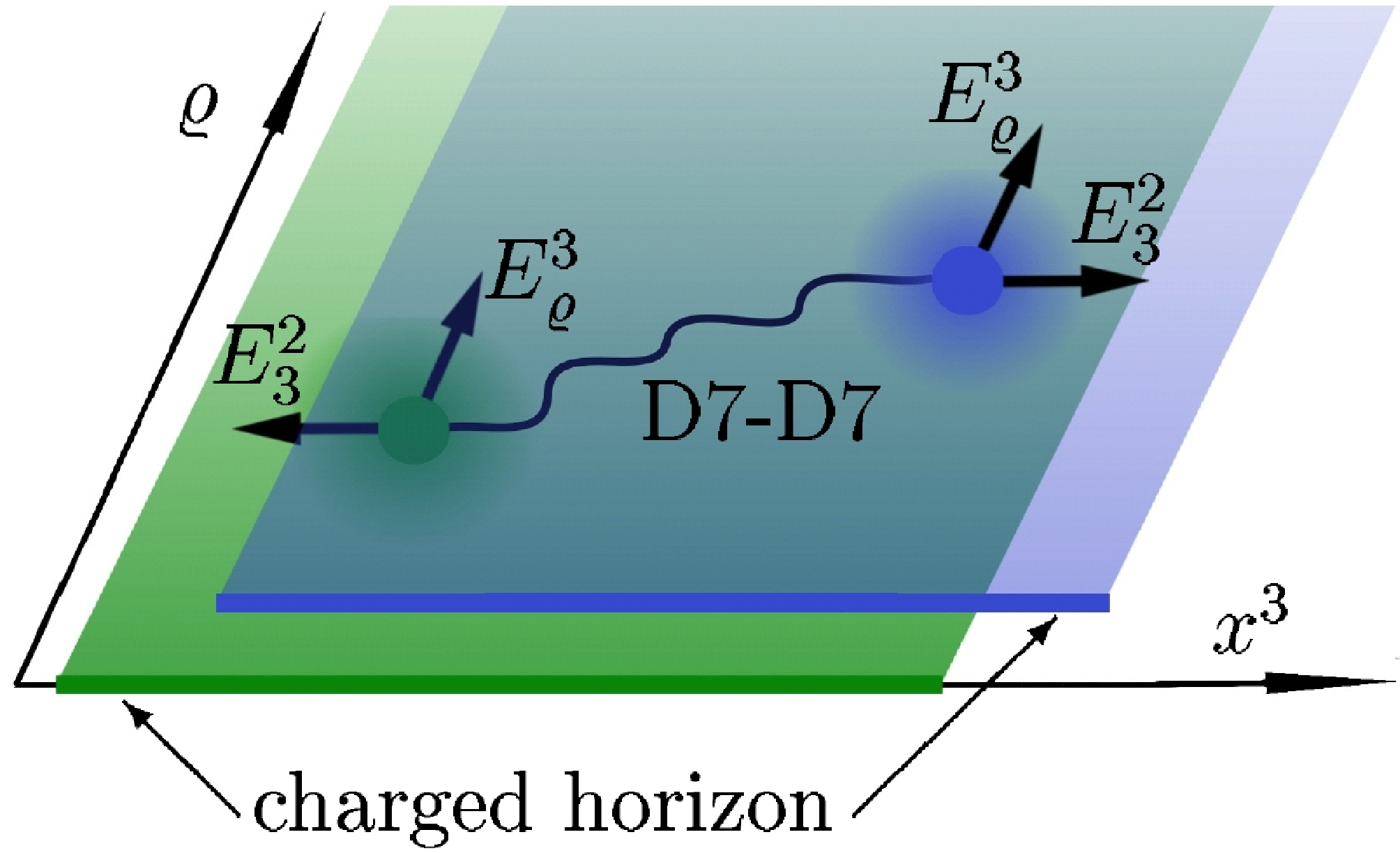
Let us first describe the unstable configuration in absence of the field . As known from [37, 31, 20], the non-zero field is induced by fundamental strings which are stretched from the D-brane to the horizon of the black hole. In the subsequent we call these strings ‘horizon strings’. Since the tension of these strings would increase as they move to the boundary, they are localized at the horizon, i. e. the horizon is effectively charged under the isospin charge given by (1). By increasing the horizon string density, the isospin charge on the D7-brane at the horizon and therefore the energy of the system grows. In [20], the critical density was found beyond which this setup becomes unstable. In this case, the strings would prefer to move towards the boundary due to the repulsive force on their charged endpoints generated by the flavorelectric field .
The setup is now stabilized by the new non-zero field . We can think of this field as being induced by D-D strings moving in the direction. This movement of the strings may be interpreted as a current in direction which induces the magnetic field . Moreover, the non-Abelian interaction between the D-D strings and the horizon strings induces a flavorelectric field .
From the profile of the gauge fields and their conjugate momenta (see figure 7) we obtain the following: For , i. e. in the normal phase (), the isospin density is exclusively generated at the horizon by the horizon strings. This can also be understood by the profile of the conjugate momenta (see figure 7 (bottom left)). We interpret as the isospin charge located between the horizon at and a fictitious boundary at . In the normal phase, the momentum is constant along the radial direction (see figure 7(bottom left)), and therefore the isospin density is exclusively generated at the horizon. In the superconducting phase where , i. e. , the momentum is not constant any more. Its value increases monotonically towards the boundary and asymptotes to (see figure 7(bottom left)). Thus the isospin charge is also generated in the bulk and not only at the horizon. This decreases the isospin charge at the horizon and stabilizes the system.
Now we describe the string dynamics which distributes the isospin charge into the bulk. Since the field induced by the D-D strings is non-zero in the superconducting phase, these strings must be responsible for stabilizing this phase. In the normal phase, there are only horizon strings. In the superconducting phase, some of these strings recombine to form D-D strings which correspond to the non-zero gauge field and carry isospin charge 99 9 Note that the D-D strings are of the same order as the horizon strings, namely , since they originate from the DBI action [37].. There are two forces acting on the D-D strings, the flavorelectric force induced by the field and the gravitational force between the strings and the black hole. The flavorelectric force points to the boundary while the gravitational force points to the horizon. The gravitational force is determined by the change in effective string tension, which contains the dependent warp factor. The position of the D-D strings is determined by the equilibrium of these two forces. Therefore the D-D strings propagate from the horizon into the bulk and distribute the isospin charge.
Since the D-D strings induce the field , they also generate the density dual to the condensate , the Cooper pairs. This density is proportional to the D-D strings located in the bulk, in the same way as the density counts the strings which carry isospin charge [31]. This suggest that we can also interpret as the number of D-D strings which are located between the horizon at and the fictitious boundary at . The momentum is always zero at the horizon and increases monotonically in the bulk (see figure 7 (bottom right)). Thus there are no D-D strings at the horizon, nevertheless most of them are located near the horizon. {svgraybox} The double importance of the D-D strings is given by the fact that they are both responsible for stabilizing the superconducting phase by lowering the isospin charge density at the horizon, as well as being the dual of the Cooper pairs since they break the symmetry. In QCD-language they correspond to quarks pairing up to form charged vector mesons which condense subsequently.
6.2 Summary
In conclusion we have derived from the top (string theory) down to the gravity theory a holographic p-wave superconductor. Thus we were able to directly identify the degrees of freedom in the boundary field theory, allowing us to translate geometric features directly into field theory features. In particular we have found a string theory picture of the pairing mechanism. The Cooper pairs are modeled by strings spanned between the two flavor D-branes corresponding to quasi-particles in the vector bi-fundamental representation, i. e. vector mesons. The dual thermal field theory is 3+1-dimensional supersymmetric Yang-Mills theory with color and flavor symmetry coupled to an gauge multiplet. It shows a conductivity gap at low temperatures. A pseudo-gap forms even above . The onset of the Meissner-Ochsenfeld effect is visible and in the conductivity spectrum we find massive quasi-particles even at vanishing quark mass. Their masses are generated through a Higgs-like mechanism in the bulk.
Note that our results can also be interpreted using this very setup as a model for the quark gluon plasma as introduced in section 3.1. In that case we have found a flavor superfluid phase. This should not be confused with the color-superconducting phase theoretically found in QCD at high baryon density.
6.3 Outlook
Some directions for promising future investigation are the study of critical exponents near the phase transition. Transport coefficients such as the speeds of second, fourth and other sounds can be determined. For some of these it will be neccessary or convenient to use the backreacted solutions for this D3/D7 system given in [49]. Similar to earlier semi-classical drag computations it might be instructive to compute the drag on the various strings near the superconducting phase transition. This computation had been suggested already in [5] and carried out for a scalar condensate superfluid in [53]. It would be interesting to see what happens to the Fermi surface formed by the background fermions when the superconducting/superfluid phase is entered. Adventurous spirits may also take this setup as a serious model for p-wave superconductors such as the ruthenate compounds mentioned in the introduction. The geometric insights we gain from the dual gravity description can in principle be directly translated to precise field theory statements. Again this pleasant fact is due to knowing the field theory degrees of freedom exactly by using the gauge/gravity correspondence. A different setup in which vector mesons condense at finite isospin potential is the Sakai-Sugimoto model as shown in [54]. It could be illuminating to study all aforementioned effects in this model as well ([55] studies a possibly superconducting phase in the Sakai-Sugimoto model but considers a pion condensate at finite baryon density).
Acknowledgements.
I thank Johanna Erdmenger for discussions as well as kind support, and Martin Ammon, Patrick Kerner, Felix Rust for fruitful collaboration. I thank Ronny Thomale for instructive discussions, and especially Christopher Herzog and Andy O’Bannon for very helpful comments on these notes. This work is supported in part by the ”Deutsche Forschungsgemeinschaft” (DFG). Last but certainly not least, I thank the organizers and participants of the Fifth Aegean Summer School ”From Gravity to Thermal Gauge Theory: The AdS/CFT Correspondence”.References
- (1) C. P. Herzog, Lectures on Holographic Superfluidity and Superconductivity, J. Phys. A42 (2009) 343001, [arXiv:0904.1975].
- (2) S. A. Hartnoll, Lectures on holographic methods for condensed matter physics, Class. Quant. Grav. 26 (2009) 224002, [arXiv:0903.3246].
- (3) G. T. Horowitz, Introduction to Holographic Superconductors, arXiv:1002.1722.
- (4) M. Kaminski, Holographic quark gluon plasma with flavor, Fortsch. Phys. 57 (2009) 3–148, [arXiv:0808.1114].
- (5) M. Ammon, J. Erdmenger, M. Kaminski, and P. Kerner, Superconductivity from gauge/gravity duality with flavor, Phys. Lett. B680 (2009) 516–520, [arXiv:0810.2316].
- (6) M. Ammon, J. Erdmenger, M. Kaminski, and P. Kerner, Flavor Superconductivity from Gauge/Gravity Duality, JHEP 10 (2009) 067, [arXiv:0903.1864].
- (7) S. A. Hartnoll, C. P. Herzog, and G. T. Horowitz, Building a Holographic Superconductor, Phys. Rev. Lett. 101 (2008) 031601, [arXiv:0803.3295].
- (8) S. S. Gubser and S. S. Pufu, The gravity dual of a p-wave superconductor, JHEP 11 (2008) 033, [arXiv:0805.2960].
- (9) S. A. Hartnoll, C. P. Herzog, and G. T. Horowitz, Holographic Superconductors, JHEP 12 (2008) 015, [arXiv:0810.1563].
- (10) G. T. Horowitz and M. M. Roberts, Holographic Superconductors with Various Condensates, Phys. Rev. D78 (2008) 126008, [arXiv:0810.1077].
- (11) S. S. Gubser, C. P. Herzog, S. S. Pufu, and T. Tesileanu, Superconductors from Superstrings, Phys. Rev. Lett. 103 (2009) 141601, [arXiv:0907.3510].
- (12) S. S. Gubser, S. S. Pufu, and F. D. Rocha, Quantum critical superconductors in string theory and M- theory, Phys. Lett. B683 (2010) 201–204, [arXiv:0908.0011].
- (13) M. et al, Superconductivity in a layered perovskite without copper, Nature 372 (1994) 532.
- (14) S. Tewari, S. D. Sarma, C. Nayak, C. Zhang, and P. Zoller, Quantum computation using vortices and majorana zero modes of a $p_x$ + $ip_y$ superfluid of fermionic cold atoms, Physical Review Letters 98 (2007) 010506.
- (15) C. Nayak, S. H. Simon, A. Stern, M. Freedman, and S. D. Sarma, Non-abelian anyons and topological quantum computation, Reviews of Modern Physics 80 (2008) 1083.
- (16) D. Vollhardt and P. Woelfle, Superfluid Phases of Helium Three. CRC Press, 1990.
- (17) I. Amado, M. Kaminski, and K. Landsteiner, Hydrodynamics of Holographic Superconductors, JHEP 05 (2009) 021, [arXiv:0903.2209].
- (18) M. Greiter, Is electromagnetic gauge invariance spontaneously violated in superconductors?, Annals of Physics 319 (2005) 217.
- (19) J. Erdmenger, N. Evans, I. Kirsch, and E. Threlfall, Mesons in Gauge/Gravity Duals - A Review, Eur. Phys. J. A35 (2008) 81–133, [arXiv:0711.4467].
- (20) J. Erdmenger, M. Kaminski, P. Kerner, and F. Rust, Finite baryon and isospin chemical potential in AdS/CFT with flavor, JHEP 11 (2008) 031, [arXiv:0807.2663].
- (21) S. S. Gubser, Breaking an Abelian gauge symmetry near a black hole horizon, arXiv:0801.2977.
- (22) S. S. Gubser, Colorful horizons with charge in anti-de Sitter space, Phys. Rev. Lett. 101 (2008) 191601, [arXiv:0803.3483].
- (23) A. Karch and E. Katz, Adding flavor to AdS/CFT, JHEP 06 (2002) 043, [hep-th/0205236].
- (24) M. Kruczenski, D. Mateos, R. C. Myers, and D. J. Winters, Meson spectroscopy in AdS/CFT with flavour, JHEP 07 (2003) 049, [hep-th/0304032].
- (25) N. R. Constable and R. C. Myers, Exotic scalar states in the AdS/CFT correspondence, JHEP 11 (1999) 020, [hep-th/9905081].
- (26) J. Babington, J. Erdmenger, N. J. Evans, Z. Guralnik, and I. Kirsch, Chiral symmetry breaking and pions in non-supersymmetric gauge / gravity duals, Phys. Rev. D69 (2004) 066007, [hep-th/0306018].
- (27) E. Witten, Anti-de Sitter space, thermal phase transition, and confinement in gauge theories, Adv. Theor. Math. Phys. 2 (1998) 505–532. hep-th/9803131.
- (28) I. Kirsch, Spectroscopy of fermionic operators in AdS/CFT, JHEP 09 (2006) 052, [hep-th/0607205].
- (29) D. Mateos, R. C. Myers, and R. M. Thomson, Holographic phase transitions with fundamental matter, Phys. Rev. Lett. 97 (2006) 091601, [hep-th/0605046].
- (30) I. Kirsch, Generalizations of the AdS/CFT correspondence, Fortsch. Phys. 52 (2004) 727–826, [hep-th/0406274].
- (31) S. Kobayashi, D. Mateos, S. Matsuura, R. C. Myers, and R. M. Thomson, Holographic phase transitions at finite baryon density, JHEP 02 (2007) 016, [hep-th/0611099].
- (32) R. C. Myers, Dielectric-branes, JHEP 12 (1999) 022, [hep-th/9910053].
- (33) A. A. Tseytlin, On non-abelian generalisation of the Born-Infeld action in string theory, Nucl. Phys. B501 (1997) 41–52, [hep-th/9701125].
- (34) A. Hashimoto and W. Taylor, Fluctuation spectra of tilted and intersecting D-branes from the Born-Infeld action, Nucl. Phys. B503 (1997) 193–219, [hep-th/9703217].
- (35) N. R. Constable, R. C. Myers, and O. Tafjord, The noncommutative bion core, Phys. Rev. D61 (2000) 106009, [hep-th/9911136].
- (36) R. C. Myers and M. C. Wapler, Transport Properties of Holographic Defects, JHEP 12 (2008) 115, [arXiv:0811.0480].
- (37) A. Karch and A. O’Bannon, Holographic Thermodynamics at Finite Baryon Density: Some Exact Results, JHEP 11 (2007) 074, [arXiv:0709.0570].
- (38) D. Mateos, S. Matsuura, R. C. Myers, and R. M. Thomson, Holographic phase transitions at finite chemical potential, JHEP 11 (2007) 085, [arXiv:0709.1225].
- (39) M. M. Roberts and S. A. Hartnoll, Pseudogap and time reversal breaking in a holographic superconductor, JHEP 08 (2008) 035, [arXiv:0805.3898].
- (40) P. Basu, J. He, A. Mukherjee, and H.-H. Shieh, Superconductivity from D3/D7: Holographic Pion Superfluid, JHEP 11 (2009) 070, [arXiv:0810.3970].
- (41) C. P. Herzog and S. S. Pufu, The Second Sound of SU(2), JHEP 04 (2009) 126, [arXiv:0902.0409].
- (42) J. Erdmenger, M. Kaminski, and F. Rust, Holographic vector mesons from spectral functions at finite baryon or isospin density, Phys. Rev. D77 (2008) 046005, [arXiv:0710.0334].
- (43) C. M. Bender and S. Orszag, Advanced mathematical methods for scientists and engineers. 1978.
- (44) D. T. Son and A. O. Starinets, Minkowski-space correlators in AdS/CFT correspondence: Recipe and applications, JHEP 09 (2002) 042. hep-th/0205051.
- (45) C. P. Herzog and D. T. Son, Schwinger-Keldysh propagators from AdS/CFT correspondence, JHEP 03 (2003) 046. hep-th/0212072.
- (46) E. Berti, V. Cardoso, and A. O. Starinets, Quasinormal modes of black holes and black branes, Class. Quant. Grav. 26 (2009) 163001, [arXiv:0905.2975].
- (47) J. Erdmenger et. al., Quasinormal modes of massive charged flavor branes, arXiv:0911.3544.
- (48) M. Kaminski, K. Landsteiner, J. Mas, J. P. Shock, and J. Tarrio, Holographic Operator Mixing and Quasinormal Modes on the Brane, JHEP 02 (2010) 021, [arXiv:0911.3610].
- (49) M. Ammon, J. Erdmenger, V. Grass, P. Kerner, and A. O’Bannon, On Holographic p-wave Superfluids with Back-reaction, arXiv:0912.3515.
- (50) E. Nakano and W.-Y. Wen, Critical magnetic field in a holographic superconductor, Phys. Rev. D78 (2008) 046004, [arXiv:0804.3180].
- (51) T. Albash and C. V. Johnson, A Holographic Superconductor in an External Magnetic Field, JHEP 09 (2008) 121, [arXiv:0804.3466].
- (52) K. Maeda and T. Okamura, Characteristic length of an AdS/CFT superconductor, Phys. Rev. D78 (2008) 106006, [arXiv:0809.3079].
- (53) S. S. Gubser and A. Yarom, Pointlike probes of superstring-theoretic superfluids, arXiv:0908.1392.
- (54) O. Aharony, K. Peeters, J. Sonnenschein, and M. Zamaklar, Rho meson condensation at finite isospin chemical potential in a holographic model for QCD, JHEP 02 (2008) 071, [arXiv:0709.3948].
- (55) A. Rebhan, A. Schmitt, and S. A. Stricker, Meson supercurrents and the Meissner effect in the Sakai- Sugimoto model, JHEP 05 (2009) 084, [arXiv:0811.3533].