On correlation functions of operators dual to classical spinning string states
Jagiellonian University
ul. Reymonta 4
30-059 Kraków
Poland
Abstract
We explore how to compute, classically at strong coupling, correlation functions of local operators corresponding to classical spinning string states. The picture we obtain is of ‘fattened’ Witten diagrams, the evaluation of which turns out to be surprisingly subtle and requires a modification of the naive classical action due to a necessary projection onto appropriate wave functions. We examine string solutions which compute the simplest case of a two-point function and reproduce the right scaling with the anomalous dimensions corresponding to the energies of the associated spinning string solutions. We also describe, under some simplifying assumptions, how the spacetime dependence of a conformal three-point correlation function arises in this setup.
1 Introduction
In a conformal field theory the full dynamical information is contained in two ingredients: the spectrum of conformal weights and the coefficients of three point functions of primary operators (OPE coefficients). All higher point correlation functions are expressible in terms of these data11 1 This has been exploited in detail for two-dimensional CFT’s [21], but should also hold for higher dimensional theories [22]..
In the case of SYM theory, thanks to the developments of integrability [1]-[10] in the AdS/CFT correspondence [11, 12, 13], we have a very detailed quantitative understanding of the structure of the spectrum of conformal weights (i.e. anomalous dimensions of operators), being very close to an explicit solution [14, 15, 16]. However, there is almost no information on the OPE coefficients apart from early works on 3-point functions of protected operators dual to supergravity modes [17, 18], short operators like Konishi [19], various operators in the BMN limit as most recently considered in [20].
This imbalance comes from the fact that in order to compute generic OPE coefficients one has to consider three point functions of primary operators which are dual to massive string states, for the calculation of which we do not have appropriate technical tools. Indeed since the calculational methods for computing correlation functions in the AdS/CFT correspondence are based on Green’s functions and an action for the corresponding fields [12, 13], they have been so far restricted to operators dual to supergravity fields. For operators dual to massive string modes, this route appears to be closed due to the absence of a workable closed string field theory in .
The main motivation for the present paper is to address this issue. Specifically, we would like to develop a setup where one may use classical (or even perhaps semi-classical) methods for computing correlation functions of operators dual to (massive) classical string states at strong coupling. In this paper we will concentrate on two-point functions, which should reproduce the known anomalous dimensions equal to the energies of the corresponding spinning string solutions in 22 2 For a stringy classical analysis of the calculation of correlation functions in the BMN limit see [23]-[25].. In addition, we will show how the standard conformal spacetime dependence of three point functions arises from the same setup. We will also describe various aspects of the calculations which were quite surprising for us.
The plan of this paper is as follows: first we will describe some motivation for the existence of a classical regime for a class of correlation functions involving massive string states, then we will proceed to review a point particle example first in flat space and then in . In section 4 we will describe various difficulties that one faces when trying to extend these calculations to the case of classical string states. In section 5 we will formulate our prescription and apply it, in the following section, to compute two point functions of operators dual to spinning string solutions. We will describe generic solutions in and a specific example with spins also in the factor. Finally, in section 7, we will describe how the spacetime dependence of a 3-point correlation function arises from this setup. We close the paper with a summary and an outlook.
2 Motivation
The conformal weights (anomalous dimensions) of gauge theory operators are extracted from the string side of the AdS/CFT correspondence by computing the energies of string states in , and using the identification between the symmetries on both sides of the correspondence. The energy of a string state in measured w.r.t. global AdS time is an eigenvalue of the operator
| (1) |
This operator is conjugate (by a nonunitary similarity transformation) to times the dilatation operator. Therefore the spectrum of conformal weights of SYM coincides with the spectrum of energies of a superstring in .
In particular, at strong coupling, there is a class of operators with large R-charges or spins which are dual to spinning string classical solutions in [26, 27, 28]. Consequently, their anomalous dimensions behave like
| (2) |
On the CFT side, we know that the two-point correlation function of the corresponding operator has to have the form
| (3) |
For consistency, it should therefore be possible to also reconstruct the same anomalous dimension from a direct computation of the correlation function (3) on the string side of the AdS/CFT correspondence. Moreover, we expect that a classical computation should suffice, as the relevant correlation function, for operators dual to spinning string states, scales as
| (4) |
at strong coupling, which is a typical form of an Euclidean action of a classical string solution. Moreover, the coefficient of should exactly coincide with the energy of the quite different Minkowskian spinning string located near the center of global . For technical reasons we will consider these correlation functions in Minkowski signature (with spacelike separation of the operator insertion points) which will be easily continued to Euclidean spacetime.
We expect, therefore, to have a mapping from classical spinning string solutions rotating around the center of Minkowskian global to certain solutions in the Poincare patch which realize the two point functions for any choice of the positions of the operator insertions on the boundary. This new classical solution should approach the boundary at exactly these points.

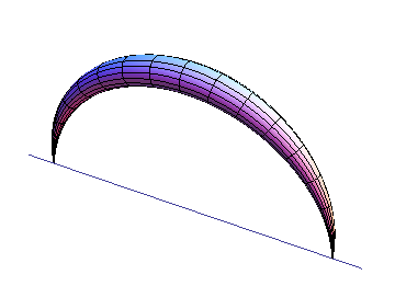
For higher point functions we may expect to have a structure of ‘fattened’ Witten diagrams [13] (shown in fig. 1 for the case of two point functions), where the type of solution approaching the relevant point on the boundary represents a kind of ‘classical’ vertex operator for the spinning string state33 3 It would be interesting to compare with [29], building upon [30].. In section 7 we will describe the spacetime structure of a three-point function in this setup.
3 A point particle example
A prototype for our considerations is the derivation of a point particle Green’s function from the worldline formalism. One can obtain the scalar field Green’s function by evaluating a path integral over the worldlines of a particle between the two points weighted with the Polyakov (particle) action and performing an integral over the modular parameter of the trajectories. This calculation has been carried out in detail in [31], here we will just discuss its classical limit. Let us start with Euclidean signature.
Then one has to perform the path integral
| (5) |
with the boundary conditions , . In the above expression, is the einbein field related to the metric on the worldline. One can use diffeomorphisms to set to a constant which becomes the modular parameter of the worldline trajectory. Equivalently, we may keep the worldline metric equal to unity and extend the range of the worldline time coordinate. In this way one gets
| (6) |
Let us now evaluate the above expression by saddle point. The solution with appropriate boundary conditions is , giving for the Polyakov action
| (7) |
Performing a saddle point w.r.t. the modular parameter gives the correct large distance asymptotics of the flat space scalar Green’s function.
| (8) |
A careful, exact evaluation of the path integral reproduces the exact scalar Green’s function [31]. Repeating the same computation in Minkowski signature, we would start from the action
| (9) |
and then, depending on whether the separation is spacelike or timelike we will arrive at a real or complex saddle point ( or ) giving the following standard asymptotics of the Feynman propagator in flat space
| (10) |
It is clear that the spacelike separation case essentially coincides with the Euclidean result.
Let us now consider the point particle in , and specialize to the case relevant for a two point function. This calculation corresponds e.g. to a heavy KK supergravity mode which is dual to a protected operator of large (classical) dimension.
For the calculation it is convenient to use the Poincare coordinates of Euclidean :
| (11) |
The two point function in the AdS/CFT correspondence is essentially the Green’s function, regularized by moving the operator insertion points by into the bulk i.e. to and with .
The relevant action for a point particle of mass is
| (12) |
where is the modular parameter of the worldline. The equations of motion in AdS are
| (13) | |||||
| (14) |
These equations are solved by
| (15) |
which is, in fact, a specific parametrization of a geodesic in . With this solution the AdS part of the action simplifies to
| (16) |
We now have to impose the boundary conditions
| (17) |
Since is very small, has to be large and we get
| (18) |
and
| (19) |
| (20) |
We now have to perform integration over the modular parameter , which we do by saddle point. The saddle point solution is
| (21) |
leading to
| (22) |
In this way we recovered the standard relation between particle
masses in and operator dimensions in the large
mass limit .
If we pass to Minkowski signature in the AdS case there are some new features in comparision to the flat space case. For spacelike separation along the coordinate, the action becomes
| (23) |
Here the solution of the equations of motion is as in the Euclidean case. The only difference is the sign of which gives rise to an imaginary saddle point in , which, when substituted back to the action compensates the prefactor in and gives the purely real answer .
For timelike separation, say along the direction, the action is
| (24) |
Now, in contrast to the flat space case, it turns out that there is no appropriate real trajectory approaching the boundary and one is forced to consider an analytically continued complex trajectory which again gives rise to the real exponent .
The obvious way to obtain the Green’s function for massive string states is to consider a cylinder amplitude for the closed string, similar to the one considered in [31, 32], and evaluate it by saddle point, ensuring that the propagating string state corresponds to a classical state with appropriate angular momenta. However it turns out that this procedure is quite subtle as we will discuss in the following section.
4 Problems with extension to strings
As a simple example which illustrates the problems encountered in extending the point particle calculation of the previous section to the closed string context, let us consider the case of the flat space cylinder amplitude described in [31, 32]. In particular, for the case of pointlike boundary conditions for the endpoints of the cylinder, the flat space amplitude (for the bosonic closed string) evaluated in Euclidean signature takes the form:
| (25) |
where is the modular parameter of the cylinder, is the classical action for a pointlike straight string stretched between point and point i.e.
| (26) |
Once we expand the product in the preexponential factor, we will get [31]
| (27) |
in which we at once recognize a summation over all string states propagating along the cylinder. Each summand is in fact just the worldline representation of the Green’s function of the corresponding string state, exactly as dicussed in the previous section. So the interpretation of each term in the cylinder amplitude is perfectly natural and in line with expectations.
Suppose now that we were to try to extract from this setup the Green’s functions of a highly excited massive string state which would be almost classical — a rotating string with large angular momenta, a typical example of which would be the following Minkowskian solution [27]:
| (28) |
supplemented by
| (29) |
It is convenient to interpret this state treating the coordinates where the rotation takes space as being in some ‘compactified’ space, while the coordinates would be the ‘physical’ ones. In this way the similarity to the setup of spinning strings in is greatest.
Once we try to extract the Green’s function corresponding to this particular solution from the cylinder amplitude, we encounter a series of difficulties. Firstly, the calculation (25) was performed in Euclidean signature, so the above solution would not be a solution of the Euclidean equations of motion. At the least it would have to be complexified, thus losing in this case any similarity with a rotating string. So suppose that to overcome this obstacle we consider the cylinder amplitude in Minkowski signature. Now at least the state (28) is a solution to the equations of motion. But then, we would expect it, being a solution to the classical equation of motion, to contribute through the exponent of the classical action in the cylinder formula. This would lead to an incorrect result as the Minkowskian action is quite different from the Minkowskian energy which is effectively responsible for the of the string state.
So let us go back to the original Euclidean formula (25) and examine more closely how the correct Green’s functions were reproduced. There, the mass terms did not arise from the classical action but rather from the fluctuation determinant. So they were associated to eigenfunctions of the Laplace operator and these, almost by chance, turned out to be related to solutions of the original Minkowskian equations of motion.
If we were to try to apply a similar Euclidean calculation to the case of , and try to extract contributions related to classical spinning strings we would fail, as we would not even have the picture of determinants and eigenfunctions since the Polyakov action in is nonlinear. Moreover we would not expect spinning string states to be associated to any kind of ‘small fluctuations’.
In the next section we will go back to Minkowskian signature and show how one does overcome the obstacles presented here. Let us emphasize that what we are after is a purely path integral derivation without any recourse to the operator formulation of the cylinder amplitude as . The reason for going this long-winded way is that we would like to obtain a (semi-)classical formulation applicable also to higher point functions and not only to the cylinder.
5 Semiclassical propagator revisited
The basic problem with obtaining the correct answer for the propagator of a certain classical string mode is that apparently, the path integral formula for a cylinder amplitude in the classical limit is necessarily dominated by
| (30) |
while the effective mass is governed not by the action but by the (classical) energy.
The resolution of this puzzle is in fact very simple, although we did not find it spelled out anywhere in the path integral literature.
Consider first a quantum mechanical system with one degree of freedom. Then, let us concentrate on a certain semi-classical state, eigenfunction of the hamiltonian, and consider its quantum time evolution. Its wave function must of course evolve according to its energy, which should be roughly, for the state in question, equal to its classical value. However, the semiclassical propagator for the system is governed only by the actions of classical trajectories. This is in essence the exact counterpart of our string cylinder puzzle.
But now, the answer is obvious. We have to convolve the semiclassical propagator with the wavefunction of the state that we are interested in. Since we are considering an almost classical state, we may use the leading WKB form of the wave function:
| (31) |
where is the action evaluated for some classical trajectory. In the classical limit we may evaluate the convolution with the wavefunction by saddle point obtaining
| (32) |
where is the initial momentum of the classical trajectory dominating the propagator. Now since consequently both and have to coincide with and of our classical state in question, the trajectory determining the propagator has to be the same as the one entering the wavefunction. The result will be
| (33) |
which can be rewritten as
| (34) |
The first two factors combine just to the standard energy phase
| (35) |
where we used the fact that the classical trajectory entering the propagator and the wavefunction have to coincide. In this way we recover the right result purely from classical (saddle point) considerations.
In the case of many degrees of freedom, one has to use the Hamilton-Jacobi equation for stationary states in order to generate the WKB wavefunction and the same reasoning goes through. The same also holds in the field theory limit.
Now its obvious that we should repeat the same procedure for the string cylinder amplitude. We should project the amplitude onto the contribution of the classical state that we are interested in by convolving with the relevant wave function. The convolution ensures that the classical solution for the cylinder should coincide with the classical state in question. Moreover, moving the wavefunction ‘across’ the cylinder will transform the contribution of that trajectory from to .
There is still one more subtlety which arises for the string cylinder amplitude. Up till now we looked at the flat space example as a product of “physical space”, where the arguments of the Green’s function are located, and “compactified space” where the string was rotating (analog of the in ). However in order to correctly extract Green’s functions of string states with nontrivial rotation also in the “physical space”, we have to subtract from the wave function the zero mode (which will enter the arguments of the Green’s function). Concretely, we will have
| (36) |
where and are the zero mode parts of the canonical momentum and velocity i.e.
| (37) |
This notion is ambiguous in spacetime and we will make a concrete proposal in this case in the following section, where we will apply the above procedure to evaluate two-point correlation functions of operators dual to spinning string states.
6 Two point correlation functions – spinning strings
Let us now analyze two point correlation functions of operators which are dual to classical spinning strings. We will first consider a string rotating in44 4 After the completion of this paper we became aware that a very similar construction for strings spinning in was performed in [33]. and then give an example of a spinning string rotating both in and in . Let us emphasize, that of course the outcome of the calculation is obvious both from the field theory point of view, and from our knowledge of the worldsheet string hamiltonian. Our objective is, however, to perform the calculation directly using purely classical methods so that the generalization of the setup to higher point correlation functions would be clear.
A simple example – circular rotating string in
Let us parametrize the metric on as
| (38) |
The simplest spinning string is the circular rotating string with two equal spins. It is contained in the subspace
| (39) |
with the nontrivial fields being
| (40) |
Here is the global AdS time, while is related to the R-charges through . The spinning string solution obeys Virasoro constraints which in this case reduce to . The global AdS energy of the solution is thus
| (41) |
Let us now compute the two point function of the corresponding gauge theory operator. As in the case of the point particle we will stay in Minkowski signature and consider the insertion points to be spacelike separated. We have to evaluate a cylinder amplitude with the Polyakov action
| (42) |
The classical solution would be a solution of the equations of motion for any value of the modular parameter with the boundary conditions
| (43) |
where we used the fact that there does not need to be any dependence for the AdS part of the solution. Therefore and are exactly given by the solutions (15). Since we are dealing with a cylinder amplitude, we do not impose Virasoro constraints. The part of the solution is just the part of the circular rotating string
| (44) |
Evaluating the Polyakov action for this configuration gives
| (45) |
However, as explained before we have to include the effect of the wavefunction of the rotating string state, which will change the action into its energy obtaining
| (46) |
Taking into account the formula for we get
| (47) |
The remaining saddle point in is just as for the case of the point particle described in section 3 and we obtain the correct two-point correlation function
| (48) |
One can check that the cylinder string solution at the (complex) saddle point in satisfies Virasoro constraints (similarly as in [34]).
Generic spinning strings on
The above analysis of the circular rotating string can be readily extended to generic spinning string states in . In this case it is convenient to write the part of (42) as
| (49) |
As for the circular string, the AdS energy (which corresponds to the anomalous dimension) of the spinning string solution is
| (50) |
where of the spinning string is related by the Virasoro constraint to the worldsheet energy of the part of the solution, namely
| (51) |
But this is exactly what we need to obtain the correct answer for the two-point correlation function. After using the wavefunction to project on the desired state, the analog of (47) becomes
| (52) |
which leads to the correlation function
| (53) |
Spinning string on
Let us now consider a more complicated example of a spinning string with angular momenta both in the and factors. Here we will have to deal with the complication that the nontrivial spinning motion of the string may interfere with the ‘bending of the solution’ necessary for the string to approach the given operator insertion points on the boundary. Also, for the same reason, finding the solution directly will not be as trivial as in the preceeding cases.
We will not consider here the most general solution but rather a simple example which exhibits all of the discussed features – a circular spinning string with [35].
The original spinning string solution has the following form in global coordinates on :
| (54) |
with the solution on being
| (55) |
Equations of motion imply . The charges55 5 Here we always extract factors of . of the solution are , and
| (56) |
The off-diagonal Virasoro constraint requires while the remaining diagonal one gives
| (57) |
which, together with (56), expresses the energy in terms of the spin .
We will now use this solution to construct an appropriate solution in the Poincare patch. We will not impose the Virasoro constraint (57) and keep arbitrary. Then we will perform the (nonunitary) transformation which exchanges with , and , and finally we will set . In this way we obtain a solution to the equations of motion which differs from (54) by , and . This solution has a very transparent meaning in Poincare coordinates:
| (58) |
It represents a rotating string “emitted” from the origin at the boundary at and propagating into the bulk with .
As a side remark, let us note that if we were to insert we would get a complex solution which has the correct value of purely imaginary eigenvalue of the dilatation operator. However, the nice spacetime picture would be lost. Going to Euclidean signature on the worldsheet would cure the behaviour in the direction but would mess up the spinning string structure. We will therefore always perform computations in Minkowski space and only take a (complex) saddle point in the final answer.
Now, in order to find the cylinder solution which approaches two given points on the boundary it is enough to perform a special conformal transformation
| (59) |
on the solution (58). Let us choose , so that the separation of the operator insertion points interferes with the rotation of the string. The resulting solution looks now more complicated with the nontrivial coordinate fields given by
| (60) |
We now have to impose the boundary conditions (43) for the string cylinder. In contrast to the examples, there will be some dependence, but since we are interested in the limit it can be neglected as we will need to have either very large or very small. Asymptotically we obtain
| (61) |
where we absorbed66 6 This seems like a very natural choice of normalization, but we do not have an intrinsic justification for it. It is nevertheless necessary for obtaining the correct answer. the into .
The classical action of this cylinder solution is
| (62) |
We now have to perform the subtraction (36). Here we face the problem that for generic curved spacetimes there is no unique way to define the zero modes, as the answer would be different in different coordinate systems. In the case of , we may however single out a prescription by requiring that it respects the symmetry of the background. So we propose to use the global coordinates to define the zero modes of the string namely
| (63) |
Due to the fact that acts linearly on the ’s, the zero mode of the transformed solution will be the transformation of the zero mode.
Let us now evaluate the correction term coming from convolution with the wavefunctions. From (36) we get
| (64) |
which gives
| (65) |
Finally, let us extremize w.r.t. . To this end we have to express the above expression in terms of physical charges of the string state. Moreover we will use (61) to evaluate the saddle point w.r.t. instead of . In this way we get for the exponent
| (66) |
The saddle point w.r.t. yields
| (67) |
which, for , exactly coincides with the Virasoro condition of the original spinning string solution (57). The cylinder amplitude at the saddle point thus gives
| (68) |
where we used the saddle point equation (67) to rewrite the answer in a form identical with the formula for the energy of the corresponding spinning string state (56).
The setup for higher point correlation functions
It is now roughly clear how in principle one should be able to compute a higher point correlation function. One should find a Minkowskian classical solution which approaches the insertion points of the operators in question with the same asymptotic behaviour as for the well-understood two point correlation functions. The legs of the string solution should be joined together somewhere in the bulk. The convolution with the wave functions should change the lagrangian into hamiltonian densitities (up to the extraction of the zero modes), but the transported wavefunctions will now be put in the vicinity of the junction point/cycle. The understanding of the structure of this string joining in , which is after all the main motivation for the present work, is a very interesting but complex problem which we leave nevertheless for future research. Finally one has to extremize w.r.t. the modular parameters and the position of the juncture.
In this paper we will just demonstrate, under some simplifying assumptions, how the standard spacetime dependence of a three point function in a conformal field theory arises from the above procedure.
7 Three point functions

Let us now consider three point correlation functions of operators dual to spinning string states rotating in . We expect a string configuration corresponding to the Witten diagram shown in fig. 2.
We will perform the calculation assuming that the solutions are undeformed away from the string junction. This should at least be true for the case of pointlike strings. In this paper we will not study the interaction vertex in more detail leaving this for future work. In particular we assume that the three external states are such that the three cylinders may be joined together at the string junction.
Let us consider the Witten diagram configuration shown in fig. 2. Each of the legs will be a cylinder solution with modular parameter extending from the point near the boundary to the string junction point . The action of the whole system will have to be extremized w.r.t. the modular parameters , as well as the coordinates of the string junction.
Using the formulas of previous sections we see that the modular parameters of the cylinders with the above boundary conditions can be expressed through the parameters of the solutions as
| (69) |
Since the ’s are independent of , instead of extremizing w.r.t. we may extremize w.r.t. . The exponent appearing in the amplitude for the three cylinders, after taking into account convolution with the wave functions is
| (70) |
Taking the saddle point w.r.t. the ’s gives
| (71) |
where we put . We now have to evaluate the parameter in terms of the boundary conditions. A quick calculation gives
| (72) |
The exponent can be further simplified to
| (73) |
where we have explicitly indicated the dependence on the insertion points. This is just a linear combination of the invariant distances between the points and weighted with the conformal dimensions of the external states77 7 This is not surprising, as from the point of view the computation becomes essentially a point-particle one.. Now we have to find the saddle point w.r.t. and . This is very difficult, if not impossible, to do explicitly. However we may use the conformal symmetry of to find the exact dependence of the answer on the positions of the operator insertion points . For simplicity we will just consider these points to lie along one coordinate axis so that the endpoints of the string cylinders are at , , , with being scalars.
Consider first the specific choice , , . The exponent will be extremized by some specific values of and :
| (74) |
Now let us take a conformal transformation which transforms the into . This induces an isometry of which transforms
| (75) |
Since the Polyakov action is invariant we have
| (76) |
where the transformed and automatically solve the saddle point equations for . But this is almost exactly what we want for the general case. Indeed, comparision with (73) gives
| (77) |
So the whole spacetime dependence sits in the last term which is easy to evaluate. In order to complete the calculation, we need the explicit form of the isometry. For the case at hand, it may be constructed from a composition of a dilatation, a special conformal transformation and a translation. Explicitly we have
| (78) | |||||
| (79) |
The parameters and are given in our case as
| (80) |
Plugging the above into (77), we obtain
| (81) |
which is the expected spacetime dependence of the three point correlation function in a conformal field theory.
8 Summary and Outlook
In this paper we have addressed the problem of computing correlation functions of operators dual to classical spinning string solutions. This can be done directly on the string side of the AdS/CFT correspondence using a classical computation. We have found that special care has to be taken when projecting on the string state in question. Convolution with semiclasssical wave functions modifies the classical action of the string solution by certain correction terms which are crucial in order to obtain the correct answer. The same methods should also apply to other versions of the AdS/CFT correspondence like [36]. It would also be interesting to investigate to what extent these methods could be extended to less symmetric examples of AdS/CFT.
We analyzed in detail the case of two point functions which are evaluated through a cylinder amplitude and a saddle point extremization w.r.t. the modular parameter. Again, the classical action has to be modified here. The two point correlation function computations, for the examples considered in the present paper, reproduce the correct scaling governed by the anomalous dimension equal to the energy of the associated spinning string state. Moreover, the string solution entering the two point correlation function computation, provides the asymptotic behaviour of classical string configurations which would enter higher point correlation functions involving the operator in question.
For the case of three point correlation functions we have shown how the expected spacetime dependence arises from our setup under some simplifying assumptions. We leave further investigation of the three point functions for future work.
The results obtained in the present paper lead to numerous directions for further research.
Even staying within the setting of two point correlation functions, it would be interesting to give a precise proof of the equivalence for all classical finite gap solutions. Also it would be very nice to develop the formulation beyond the strict classical limit and include quadratic fluctuations. This might be especially interesting for short operators, like Konishi, where the formulation involving fluctuations around a geodesic close to the boundary seems to be quite distinct from a short string living in the center of in an almost flat geometry. This point of view might thus lead to a cross check of the currently available string computations at strong coupling [37, 38] and the fit to numerical Y-system results [39].
The most interesting further directions to explore would be connected with the understanding of the classical solutions associated with three point correlation functions. These would have the topology of a sphere with three holes (effectively punctures in the limit). The solutions in the vicinity of these punctures should approach the operator insertion points on the boundary with the asymptotic behaviour characteristic of the given operator, which can be read off from the known two point correlation function solution. The properties and conditions for the existence of such solutions remain, for the moment, a completely open problem. However, the machinery of integrability should certainly be applicable here.
Acknowledgments: This work was supported by Polish science funds as research projects N N202 105136 (2009-2011) (RJ and PS), N N202 239637 (PS) and N N202 126735 (2008-2010) (AW). RJ was supported by Marie Curie ToK KraGeoMP (SPB 189/6.PRUE/2007/7). RJ thanks IPMU, Tokyo and IPhT Saclay for hospitality and support during work on this project. PS thanks Max-Planck-Institut für Physik in Munich for hospitality and support during the completion of this work. RJ would like to thank Sergey Frolov and Ryo Suzuki for interesting discussions. Finally, we thank Arkady Tseytlin for comments and informing us of Ref. [33].
References
- [1] I. Bena, J. Polchinski and R. Roiban, “Hidden symmetries of the AdS(5) x S**5 superstring,” Phys. Rev. D 69 (2004) 046002, [hep-th/0305116].
- [2] J. A. Minahan and K. Zarembo, “The Bethe-ansatz for N = 4 super Yang-Mills,” JHEP 0303, 013 (2003), [hep-th/0212208].
- [3] V. A. Kazakov, A. Marshakov, J. A. Minahan and K. Zarembo, “Classical / quantum integrability in AdS/CFT,” JHEP 0405, 024 (2004) [arXiv:hep-th/0402207].
- [4] N. Beisert, V. Dippel and M. Staudacher, “A novel long range spin chain and planar N = 4 super Yang-Mills,” JHEP 0407, 075 (2004) [hep-th/0405001].
- [5] G. Arutyunov, S. Frolov and M. Staudacher, “Bethe ansatz for quantum strings,” JHEP 0410, 016 (2004) [arXiv:hep-th/0406256].
- [6] N. Beisert and M. Staudacher, “Long-range PSU(2,24) Bethe ansaetze for gauge theory and strings,” Nucl. Phys. B 727, 1 (2005) [hep-th/0504190].
- [7] N. Beisert, “The su(2—2) dynamic S-matrix,” Adv. Theor. Math. Phys. 12, 945 (2008) [arXiv:hep-th/0511082].
- [8] R. A. Janik, “The AdS(5) x S**5 superstring worldsheet S-matrix and crossing symmetry,” Phys. Rev. D 73, 086006 (2006) [arXiv:hep-th/0603038].
- [9] N. Beisert, R. Hernandez and E. Lopez, “A crossing-symmetric phase for AdS(5) x S**5 strings,” JHEP 0611, 070 (2006) [arXiv:hep-th/0609044].
- [10] N. Beisert, B. Eden and M. Staudacher, “Transcendentality and crossing,” J. Stat. Mech. 0701, P021 (2007) [arXiv:hep-th/0610251].
- [11] J. M. Maldacena, “The large N limit of superconformal field theories and supergravity,” Adv. Theor. Math. Phys. 2, 231 (1998) [Int. J. Theor. Phys. 38, 1113 (1999)] [arXiv:hep-th/9711200].
- [12] S. S. Gubser, I. R. Klebanov and A. M. Polyakov, “Gauge theory correlators from non-critical string theory,” Phys. Lett. B 428, 105 (1998) [arXiv:hep-th/9802109].
- [13] E. Witten, “Anti-de Sitter space and holography,” Adv. Theor. Math. Phys. 2, 253 (1998) [arXiv:hep-th/9802150].
- [14]
G. Arutyunov and S. Frolov,
“String hypothesis for the mirror,”
JHEP 0903, 152 (2009)
[arXiv:0901.1417 [hep-th]];
G. Arutyunov and S. Frolov, “Thermodynamic Bethe Ansatz for the Mirror Model,” JHEP 0905 (2009) 068 [arXiv:0903.0141 [hep-th]],
G. Arutyunov, S. Frolov and R. Suzuki, “Exploring the mirror TBA,” arXiv:0911.2224 [hep-th]. - [15]
N. Gromov, V. Kazakov and P. Vieira,
“Integrability for the Full Spectrum of Planar AdS/CFT,”
arXiv:0901.3753 [hep-th];
N. Gromov, V. Kazakov, A. Kozak and P. Vieira, “Integrability for the Full Spectrum of Planar AdS/CFT II,” arXiv:0902.4458 [hep-th]. - [16] D. Bombardelli, D. Fioravanti and R. Tateo, “Thermodynamic Bethe Ansatz for planar AdS/CFT: a proposal,” arXiv:0902.3930 [hep-th].
- [17] D. Z. Freedman, S. D. Mathur, A. Matusis and L. Rastelli, “Correlation functions in the CFT()/AdS() correspondence,” Nucl. Phys. B 546, 96 (1999) [arXiv:hep-th/9804058].
- [18] G. Arutyunov and S. Frolov, “Some cubic couplings in type IIB supergravity on AdS(5) x S(5) and three-point functions in SYM(4) at large N,” Phys. Rev. D 61, 064009 (2000) [arXiv:hep-th/9907085].
- [19] M. Bianchi, S. Kovacs, G. Rossi and Y. S. Stanev, “Properties of the Konishi multiplet in N = 4 SYM theory,” JHEP 0105 (2001) 042 [arXiv:hep-th/0104016].
- [20] G. Georgiou, V. L. Gili, R. Russo, ”Operator mixing and three-point functions in N=4 SYM,” JHEP 10 (2009) 009 [arXiv:0907.1567]
- [21] A. A. Belavin, A. M. Polyakov and A. B. Zamolodchikov, “Infinite conformal symmetry in two-dimensional quantum field theory,” Nucl. Phys. B 241, 333 (1984).
- [22] E. S. Fradkin and M. Y. Palchik, “New developments in D-dimensional conformal quantum field theory,” Phys. Rept. 300 (1998) 1.
- [23] S. Dobashi, H. Shimada and T. Yoneya, ”Holographic Reformulation of String Theory on background in the PP-wave limit,” Nucl. Phys. B 665, 94 (2003) [arXiv:hep-th/0209251]
- [24] T. Yoneya, ”What is Holography in the Plane-Wave Limit of AdS/CFT Correspondence?” Prog. Theor. Phys. Suppl. 152, 108 (2004) [arXiv:hep-th/0304183]
- [25] S. Dobashi, T. Yoneya, ”Resolving the Holography in the Plane-Wave Limit of AdS/CFT Correspondence,” Nucl. Phys. B 711, 3 (2005) [arXiv:hep-th/0406225]
- [26] S. S. Gubser, I. R. Klebanov and A. M. Polyakov, “A semi-classical limit of the gauge/string correspondence,” Nucl. Phys. B 636, 99 (2002) [arXiv:hep-th/0204051].
- [27] S. Frolov and A. A. Tseytlin, “Multi-spin string solutions in AdS(5) x S**5,” Nucl. Phys. B 668, 77 (2003) [arXiv:hep-th/0304255].
- [28] For a review see A. A. Tseytlin, “Spinning strings and AdS/CFT duality,” arXiv:hep-th/0311139.
- [29] E. I. Buchbinder, “Energy-Spin Trajectories in from Semiclassical Vertex Operators,” arXiv:1002.1716 [hep-th].
- [30] A. A. Tseytlin, “On semiclassical approximation and spinning string vertex operators in AdS(5) x S(5),” Nucl. Phys. B 664, 247 (2003) [arXiv:hep-th/0304139].
- [31] A. G. Cohen, G. W. Moore, P. C. Nelson and J. Polchinski, “An Off-Shell Propagator For String Theory,” Nucl. Phys. B 267, 143 (1986).
- [32] A. V. Marshakov, “The path integral representation of fermionic string propagator,” Nucl. Phys. B 312, 178 (1989).
- [33] A. Tsuji, “Holography of Wilson loop correlator and spinning strings,” Prog. Theor. Phys. 117, 557 (2007) [arXiv:hep-th/0606030].
- [34] K. Zarembo, “Wilson loop correlator in the AdS/CFT correspondence,” Phys. Lett. B 459, 527 (1999) [arXiv:hep-th/9904149].
- [35] G. Arutyunov, J. Russo and A. A. Tseytlin, “Spinning strings in AdS(5) x S**5: New integrable system relations,” Phys. Rev. D 69, 086009 (2004) [arXiv:hep-th/0311004].
- [36] O. Aharony, O. Bergman, D. L. Jafferis and J. Maldacena, “N=6 superconformal Chern-Simons-matter theories, M2-branes and their gravity duals,” JHEP 0810 (2008) 091 [arXiv:0806.1218 [hep-th]].
- [37] G. Arutyunov and S. Frolov, “Uniform light-cone gauge for strings in AdS(5) x S**5: Solving su(1—1) sector,” JHEP 0601, 055 (2006) [arXiv:hep-th/0510208].
- [38] R. Roiban and A. A. Tseytlin, “Quantum strings in : strong-coupling corrections to dimension of Konishi operator,” JHEP 0911, 013 (2009) [arXiv:0906.4294 [hep-th]].
- [39] N. Gromov, V. Kazakov and P. Vieira, “Exact AdS/CFT spectrum: Konishi dimension at any coupling,” arXiv:0906.4240 [hep-th].