Correlations in impact-parameter
space
in a hierarchical saturation model
for QCD at high energy
Abstract
In order to get an estimate of the homogeneity of the distribution of matter in a fast hadron or nucleus, we compute the correlations of the saturation scales between different points in impact-parameter space, in some specific saturation models. We find that these correlations are quite strong: The saturation scale is nearly uniform in domains whose sizes scale like , which means that the density of gluons should not fluctuate significantly over regions of that typical size. We expect these conclusions as well as the explicit analytical expressions we obtain for the correlations to be true also for full QCD in appropriate limits.
1 Introduction
In the high-energy regime of QCD, an interesting new phenomenon is expected to show up: parton saturation [1, 2]. Saturation changes qualitatively the usual equation for the evolution of scattering cross sections with the energy of the reactions, namely the so-called Balitsky-Fadin-Kuraev-Lipatov (BFKL) equation [3], by introducing nonlinearities. In turn, due to these nonlinearities, the intrinsic stochasticity of partonic evolution may start to have a sizable effect on observables.
The basic nonlinear evolution equation beyond the linear BFKL equation is the Balitsky-Kovchegov (BK) equation [4, 5] (or, alternatively, the Balitsky-Jalilian Marian-Iancu-McLerran-Weigert-Leonidov-Kovner (B-JIMWLK) equations [4, 6]) which however neglects the stochastic effects alluded to before, and is therefore a kind of mean-field approximation. While a formulation which would include all stochastic effects has not been fully achieved yet (the most recent advances may be found in Ref. [7]), it is believed that the complete evolution has a lot in common with some reaction-diffusion processes described by equations of the Fisher-Kolmogorov-Petrovsky-Piscounov (FKPP) type [8]. At the mean-field level, this analogy is a formal identity between the FKPP equation and the BK equation in the so-called diffusive limit and assuming uniformity in the transverse space (i.e. the gluon distribution is assumed to evolve in the same way at all points of the impact-parameter space) [9]. Beyond the mean-field approximation, the conjecture made so far for the full problem is that at any fixed position in transverse space, the rapidity evolution of say the gluon content of a hadronic object is like the time evolution of a one-dimensional reaction-diffusion process, whose space variable would be the logarithm of the transverse size (or momentum) of the gluons. Generally speaking, the dynamics of such systems is described by equations equivalent to stochastic extensions to the FKPP equation. (The first ideas on how to go beyond the BK equation were presented in Ref. [10]; the equivalence with reaction-diffusion processes was conjectured in Ref. [11]; deeper insight can be found in e.g. Ref. [12], and a review in Ref. [13].)
While this analogy is useful to find asymptotic properties of observables that involve one unique impact parameter, so far little is known about the correlations and the fluctuations of the gluon distribution between different points in transverse space, which would show up in observables that probe several points in impact-parameter space simultaneously.
The correlations of the gluon number densities at different points in transverse space were computed exactly in Ref. [14] in the context of the systematic approximation to full QCD provided by the color dipole model [15], which is an accurate representation of the physics described by the BFKL equation but which does not take into account saturation effects. In Ref. [16], a calculation was done in a theory with full saturation based on a similarity with the Liouville gravity. But that calculation was valid only up to distances of the order of the inverse saturation momentum. On the numerical side, on one hand, the BK equation was solved taking into account the full impact-parameter dependence [17], and on the other hand, the relevance of the one-dimensional stochastic FKPP equation at each fixed impact parameter was tested in toy models for QCD evolution beyond the mean-field approximation [18].
In this paper, we would like to investigate how the saturation scale varies in impact-parameter space in the presence of both saturation and fluctuations. Our method will consist in proposing a simple toy model which contains the main physical features of QCD, which may be implemented as a Monte-Carlo event generator and for which analytical calculations will be possible. In these respects, our approach follows the one developed in Ref. [18], but while the latter work was purely numerical, our main results will consist in analytical expressions of the correlation of the saturation scale between two points in impact-parameter space, as a function of the distance between the points and as a function of the rapidity.
The model is introduced in the next section. We then provide the derivation of the analytical expression for the correlations. Finally, we check our calculations against numerical simulations of different versions of the model.
2 Toy model
2.1 Construction
The model that we introduce here is a simplified version of the model proposed in Ref. [18].
The starting point is the QCD color dipole model [15], supplemented with some ad hoc saturation mechanism which limits the number of dipoles in any given phase space cell. The dipole model accurately represents the QCD evolution in the high-energy regime and in the limit of a large number of colors. It provides an equation for the change of the density of gluons (represented by a set of color dipoles of different sizes and positions in the two-dimensional plane transverse to the flight axis of the hadron) inside a hadron, when rapidity is increased. The basic process from which the evolution is built is the splitting of a dipole represented by its two endpoints into two dipoles and with the rate [15]
| (1) |
As usually, , where is the strong coupling constant, the number of colors and is the rapidity. The splitting of dipoles is a linear process, which generates the BFKL equation when averages over dipole configurations (“events” in an experimental language) are taken. The rapidity is an effective evolution time.
When the rapidity becomes very high, then gluons and thus dipoles may start to interact among themselves, which induces nonlinear terms in the evolution equations. The effect of these interactions is to tame the growth of the phase-space number density of dipoles as soon as it reaches , which would otherwise be exponential with the rapidity. The precise mechanism for these effects is still not known in QCD, but the main observables should be quite independent of these details.
With respect to QCD, we assume the following simplifications: (i) Dipoles evolve by giving birth to one dipole of half size (the left or the right half of the parent dipole), or to one dipole of double size (in such a way that the parent be the left or right half of its offspring) at some fixed rates, (ii) dipoles do not disappear in the evolution, that is to say, the parent dipoles are not removed, (iii) the positions and dipole sizes are discrete, and (iv) the configuration space of the dipoles is a line instead of the full two-dimensional space. We thus give up two main properties of the QCD dipole model: The collinear singularities, which cause the dipole endpoints to emit an arbitrary number of dipoles of arbitrarily small sizes, and the continuous and two-dimensional nature of the dipole sizes and positions. The first simplification is the diffusion approximation, which has been studied in the context of BFKL physics (see e.g. Ref. [19]), but which was not assumed in Ref. [18]. The second simplification was instead already assumed in [18]. These model simplifications may introduce some artefacts, but that we believe are under control, and many results which we will obtain within such simple models are likely to apply to QCD since they will not depend on the details.
Let us now specify completely the model. According to the evolution rules given above, starting from a dipole of size 1, the sizes of all dipoles present in the system after evolution are powers of 2. In practice, we shall only consider fractions of 1, i.e. the sizes may be written as , where . For each value of , there are possible values of the position of the center of the dipoles: . Let us number these bins by the index running from the negative to the positive positions. The model may be represented as a hierarchy of bins that contain a discrete number of dipoles, see Fig. 1. Note that to any given impact parameter between and corresponds one unique bin at each level of size. For example, at position , one sees the bins , , etc… At position , one sees the bins , , etc… More generally, at position , one sees , where the square brackets represent the integer part.
During the rapidity (or time) interval , a dipole in the bin has a probability to give birth to a dipole in the bin , to give a dipole in the bin , and to give a dipole in the bin if is even and if is odd. Note that may be infinitesimal (which is generally speaking convenient for analytical calculations), but also finite (which is convenient for numerical simulations).
As for the saturation mechanism, we assume the simplest one: We veto splittings to bins which already host the number of dipoles.

We can consider that the number density of “gluons” of a given size seen at one impact parameter is proportional to the number of dipoles in the corresponding bin . As rapidity is increased, the occupation of the bins with low values of gets higher until the number of objects they contain reaches . The subsequent filling of the bins indexed by larger values of (smaller dipole sizes) can be seen as the propagation of traveling wave fronts at each impact parameter, with possibly complicated relationships between them. The (logarithm of the) saturation scale at impact parameter is related to the position of the front seen there at time . There are several equivalent ways to define the position of the front. It could be, for example, the largest value of for which the number of objects becomes some given fraction of . (Later, we will use a slightly different definition).
2.2 Basic features of the model
Let us denote by the number of dipoles present in bin at time . Then, according to the rules given above, we can write the following stochastic evolution equation:
| (2) |
where the are drawn according to the binomial distribution
| (3) |
This is a rather complicated equation which we do not know how to solve except numerically.
This model does not a priori look like a stochastic FKPP model. We may assume uniformity in impact parameter: This would amount to imposing the same and respectively for all at any given . In this case, the model would be projected to the FKPP class, but by definition, this would wash out the fluctuations between the different impact parameters. This simplified model, that we call “FIP” (for “Fixed Impact Parameter”, since effectively, the model is completely defined by a single impact parameter) in the terminology of Ref. [18], is nevertheless useful since it provides a benchmark to evaluate how the fluctuations between different impact parameters may alter the FKPP picture. In this paper, we will rely on (and check again in the case of our model) the conclusion reached in Ref. [18] that thanks to saturation, locally at each impact parameter, the full model is still well-described by a one-dimensional FKPP equation, and the fluctuations between different positions in impact-parameter space do not qualitatively change the picture.
Let us first apply the well-known treatment of FKPP equations to the FIP case. We know that the large-rapidity realizations of the model are stochastic traveling waves, whose main features can be determined from a simple analysis of the linear part of the evolution equation. In this model, only the number of dipoles in the bins say (i.e. at impact parameter ) is relevant. The evolution equation reads11 1 We could also write instead of the last term in Eq. (4). (This may even be a more literal implementation of the FIP approximation). But this would not make a large difference, which anyway, we would be unable to capture analytically.
| (4) |
The mean-field (or Balitsky-Kovchegov) approximation to the evolution leads to the equation
| (5) |
where the are now real functions of . The linearized equation (equivalent to the BFKL equation) is simply obtained by discarding the “” in the previous equation:
| (6) |
From standard arguments, we know that for asymptotically large and , the velocity of the wave front, that is the time derivative of the position of the front, is given by [8, 1, 20, 21]
| (7) |
where is the eigenvalue of the kernel of the linearized evolution equation (6) corresponding to the eigenfunction , namely
| (8) |
and minimizes . We recall that may be finite or infinitesimal, in which case Eq. (8) is to be understood as the derivative of . The shape of the front is a decreasing exponential to the right of the saturation region,
| (9) |
extending to for large times.
The corrections due to the discreteness of are known. Taking the latter into account, the front has now a finite extension, of the order of
| (10) |
Indeed, typically, it cannot extend further than the point where , and Eq. (10) then follows from Eq. (9). Its mean velocity reads [22, 10]
| (11) |
This velocity was obtained in a still deterministic (mean-field) approximation with appropriate cutoffs to mimic saturation and discreteness. Taking furthermore fluctuations into account, the velocity becomes [23]
| (12) |
and realization-to-realization fluctuations are characterized by the following cumulants of the position of the front:
| (13) |
where a priori the model leads to , but empirically, a better fit to the results of the numerical simulations is obtained by adding a subleading correction of the form . In particular, the diffusion constant of the front, that is to say the slope of the -dependence of the second-order cumulant reads
| (14) |
These expressions are valid in the limit of large , i.e. for exponentially large values of .
There exists a subclass of these models that may be reduced exactly to a collection of FKPP models. Let us set , that is to say, authorize only splittings to smaller-size dipoles. Consequently, there may not be any influence of the bins at any size level on the content of the bins of level less than (i.e. of larger sizes). Then, at each impact parameter, one has a FIP model, i.e. a model of the one-dimensional FKPP type. However, the relationship between the different copies of FIP models is not trivial, since part of the evolution is common between different impact parameters. Even for , we believe that this minimal model, consisting in considering two one-dimensional systems appropriately correlated, is a good approximation to the full model.
In our investigations, we will have in mind the latter class of models, and we will check numerically that for more general models for which , the results that we shall obtain are not significantly altered.
3 Correlations in the hierarchical model
Our aim is to study the correlations between the point at position in transverse space (left edge of the system, see Fig. 1) and the one at position with . We calculate the average of the squared difference of the positions of the front between these points, which is formally related to the two-point correlation function of (the logarithm of) the saturation scales, and which we deem a good estimator of the spatial fluctuations of the saturation scale. In the hierarchical model, all bins with index less than or equal to (the notation “” stands for the integer part) and overlap both impact parameters, and thus the dipoles of size larger than seen at these points are exactly the same. For instead, the bins seen at the two points are distinct and nonoverlaping. So in particular, in our model with , as soon as the position of the front at one point or at the other is larger than , that is to say, as soon as there are of the order of dipoles in the bin , then the evolutions are completely uncorrelated at the two points in the corresponding bins. (We expect that for finite of order 1, the discussion would not be qualitatively changed.) This matches to the picture that we may infer for the QCD dipole model: The dipoles at two positions in impact-parameter space separated by a distance larger than the typical saturation scales in that region evolve (almost) independently towards larger rapidities. Note that choosing pairs of points around impact parameter 0, one with positive impact parameter and another one with negative impact parameter, would not satisfy this property, due to the rigidity of the sizes and positions of the dipoles. Indeed, these two points would decorrelate very soon in the evolution since their common ancestors necessarily sit in the bin , see Fig. 1.
As a consequence of these features of QCD reproduced in the toy model, studying two-point correlations between points in impact-parameter space as a function of their distance and of the time (=rapidity) is equivalent to studying the time dependence of the correlations of the saturation scales of two realizations of the model whose evolutions are identical until the tip of the front reaches . On the average, it takes a time , being the mean velocity of the individual fronts, for the front whose tip is at at the beginning of the evolution to have its tip at . Then the bins such that evolve independently between the two realizations over the remaining time interval
| (15) |
Note that this is very close to assuming that the realizations are identical for and completely uncorrelated for .
From this discussion, we see that the basic input of our calculation will be the mechanism for the propagation of a FKPP front. We will review it in the next subsection, then we will proceed to the formulation of the calculation of the correlations.
3.1 Short review of the mecanism for stochastic front propagation
In this section, we review the recent progress in the understanding of the mecanism for front propagation [22, 10, 23], which has eventually led to the formulation of a model, and from which Eqs. (12), (13) follow [23].
Instead of solving the nonlinear problem, it was proposed [22, 10] to replace the nonlinearities by absorptive boundaries, and to treat the evolution equation as a linear (branching diffusion) equation between these boundaries. There are two types of nonlinearities: (i) The saturation condition that keeps the number of particles in each bin less than or equal to and (ii) the very discreteness of this number of particles, whose effect mainly shows up in the region where . The position of the boundaries is adjusted in such a way that the distance between them be the size of the front (10), namely , and that the large-time solution of the diffusion equation be stationary. This procedure leads to the expression of the front velocity for large given in Eq. (11), but it does not predict the fluctuations of the position of the front.
In order to incorporate the latter, we add to this picture the possibility that there be one (or a few) particles randomly sent ahead of the tip of the front [23], at a distance . We attribute to this event a probability per unit time
| (16) |
in the continuation of the shape of the front (9) solution in the large- and large- limit. ( is some constant, undetermined at this stage). In Ref. [23], we treated such fluctuations as localized extra weights of appropriate “mass” a unit or so to the left of the right boundary. We then computed the effect of this weight on the position of the front at large time, and found a forward shift of the position equal to
| (17) |
is another constant. At large times after a fluctuation has occurred, the front relaxes to its mean-field shape. We assumed that the relevant fluctuations are rare enough in such a way that the front has time to completely relax between two fluctuations, which turns out to be true for .
From the two quantitative elements (16) and (17), together with the solution of the stationary diffusion problem between the boundaries (11), we may write down an effective theory for stochastic front propagation, with however two unknown parameters, namely and . While we were not able to determine and separately, it is the product that appears in all cumulants of the position of the front, and in particular in the correction to the velocity induced by fluctuations. Assuming that the velocity of the front taking into account the fluctuations is the velocity of a mean-field front whose size is extended by with respect to (i.e. with the substitution ), we got a determination of the product :
| (18) |
The effective theory for front propagation then leads to Eqs. (12) and (13). As we will see below, the only new ingredient that will be needed is the time dependence of the shift of the front , whose large-time asymptotics is Eq. (17).
3.2 Formulation of the calculation of correlations
In line with the above discussion, we wish to compute the correlations of the position of two fronts whose evolutions are identical for and uncorrelated for . Note that strictly speaking, we would need to keep the content of all bins identical between the two realizations at all times, even after time . But these two formulations give quantitatively similar results.
Let us introduce the position of the front at time in the frame in which . We focus on what happens slightly before the initial time . On one hand, if no fluctuation has occurred between times and , on the other hand, if a fluctuation has occurred at a position ahead of the front (which happens with probability ). It is straightforward to write an equation for the generating function of the cumulants of :
| (19) |
One now considers two such independent fronts and add up the generating functions. One gets
| (20) |
Expanding for close to 0, the coefficients of the second power of obey the equation
| (21) |
where we have used the fact that and are independent random variables for , and we have traded for in the derivative, taking advantage of the fact that both and only depend on . In practice, will be equal to , the time at which the tip of the single front reaches . From Eq. (15), this time is .
3.3 Effect of a fluctuation on the position of the front
The problem amounts to solving a diffusion equation between two fixed absorptive boundaries, with various initial conditions. We shall discuss the scaled dipole number , and for the simplicity of the formalism, consider that it is a function of a real variable .
Let us write the general branching diffusion equation:
| (22) |
where is an appropriate kernel that encodes the linear evolution of the dipoles. (The operators that appear here are denoted as differential operators, but they could also be finite differences as in Eq. (6). Analytical calculations are usually easier with differential operators). In the case of QCD, would be the BFKL kernel (that can easily be deduced from Eq. (1)), , (where is the size of the dipoles), and would be the scattering amplitude. Further, we define to be the eigenvalue of that satisfies . Following Ref. [23], we write the ansatz
| (23) |
is the size of the front, which is essentially for large . When is expanded to second order around the eigenvalue , then obeys the partial differential equation
| (24) |
where we have defined
| (25) |
We have only kept the dominant terms for large . We see that has to scale like for all terms of this equation to be relevant. The coefficient must be chosen in such a way that in the large- limit, there is a nontrivial stationary solution. We shall use the already known result (11) to write
| (26) |
and check a posteriori that it is the correct expression. Equation (24) then becomes
| (27) |
up to higher-order terms when is large.
We shall admit that the saturation of the number of dipoles and the stochasticity may be appropriately implemented, within well-controlled approximations, by respectively an absorptive boundary at and another one at (which corresponds to a distance between the boundaries in -coordinates, i.e. to the natural width of the stationary front which travels at the velocity ). The boundary conditions formally read
| (28) |
Let us now discuss the initial condition. The fluctuations that will generate the front-shifts responsible for the corrections to are dipoles sent at a distance ahead of the tip of the steady front. Formally, in order to describe such a fluctuation occurring at time , we would write , i.e. from Eq. (23), . But since there is an absorptive boundary at , we had better move the fluctuation to the left of the right boundary. This should not qualitatively change the problem as long as . Thus we write
| (29) |
where is a constant of order , and therefore .
The solution of Eq. (27) with the conditions (28) and (29) reads
| (30) |
The subscript recalls that this solution was obtained starting with an initial condition consisting in one dipole at a distance ahead of the deterministic front.
We first discuss the stationary solution. We see that for large , the higher harmonics are suppressed exponentially with respect to the fundamental mode , which gives the following contribution:
| (31) |
Thanks to the choice (26) for , this solution has no dependence, and leads to a stationary in the frame of the front. The expression (31) is independent of the initial condition except for the overall normalization. The value of , which characterizes the initial condition, will be adjusted later. Undoing the changes of variables which trade for , for and for (Eq. (23)), the stationary solution reads
| (32) |
We require that for , where is a constant of order 1. This condition is satisfied if we set . Indeed, with this choice,
| (33) |
Since and are constants, the right-hand side is just a number of order 1.
We now add a fluctuation to the stationary front, that is to say, an extra particle at a position ahead of the tip of the steady front. The solution of the diffusion equation is the superposition of the large-time stationary solution given by Eq. (32) with , and of the solution of the diffusion equation with the generic initial condition characterized by (see Eq. (30)), up to a multiplicative constant of order 1 that we do not control in this calculation, since it certainly depends on the detailed shape of the fluctuations. We write
| (34) |
up to the replacement of the variables by their expressions (25).

The presence of the second term alters the shape of the front (the front eventually relaxes back to the sine shape in Eq. (32)), see Fig. 2. But of course, we want to keep the normalization condition for , namely for some appropriate value of , is required to equate Eq. (33) at all . This is possible by shifting the value of at which we enforce the normalization condition from to say . This is equivalent to shifting the position of the front . Equation (34) then leads to
| (35) |
Equating the right-hand sides of Eq. (35) and Eq. (33), we get
| (36) |
where only the lowest orders in , in the expansion of must be kept. With the help of Eq. (30), it is then straightforward to arrive at an explicit expression of .
Note that by performing the shift , we have actually added a -dependent term to in Eq. (26), which was initially assumed to be a constant. However, since the time scale for the variations of is , is suppressed for large , and thus Eq. (27) is not modified within our approximations.
It is interesting to note that is related to some Jacobi function [24]. Since
| (37) |
we may rewrite Eq. (30) as
| (38) |
The notation
| (39) |
has been introduced. Using Eq. (36) and performing the appropriate expansion for small and , we arrive at an expression for in terms of the -function which is particularly compact:
| (40) |
with
| (41) |
It is actually quite natural that the Jacobi theta functions appear, since the latter are defined as solutions of the one-dimensional heat equation with periodic boundary conditions.
We turn to the analysis of the obtained result. First, for large , only the fundamental mode contributes to , and it is clear that Eq. (36) reduces to Eq. (17). Looking back at Eq. (30), we see that higher harmonics would give a series of exponentially decreasing corrections. But at a finite time, a large number of modes have to be taken into account, typically all modes such that . A few low-lying modes are not enough to describe the small-time behavior. Instead, it is a saddle point (in an appropriate integral reformulation) that dominates the sum (30). In this regime, it would be useful to find a way to write the series of harmonics such that at asymptotically large , only the first term contributes instead of the whole series. This is actually possible using the Poisson summation formula
| (42) |
In order to get , we need the value of at . Hence we choose
| (43) |
We then perform the integral over in the r.h.s. of Eq. (42). Introducing and , we get the following expression for :
| (44) |
Since we eventually want to apply Eq. (36) in order to get an expression of the shift of the front, we expand the latter formula for . The leading order reads
| (45) |
The shift of the front due to a fluctuation is obtained from with the help of Eq. (36):
| (46) |
is the function of given by Eq. (39). This formula is extremely useful, since the series indexed by converges fast. Even for moderately large values of , a few terms accurately describe the whole function. This is actually the best formula for numerical evaluations of .
We shall now examine the limit of small (). Then only the term has to be kept. The expression for boils down to
| (47) |
3.4 Analytical expression for the correlations
With the elements presented in the previous sections, we can write the expression for . It is enough to insert the expression for the probability of fluctuations (Eq. (16)) and for the time-dependent shift (Eq. (40)) into Eq. (21):
| (49) |
where for we use either one of the equivalent expressions (41), (48) according to the limit that we want to investigate. We now have to fix the value of . In Ref. [23], was taken to be a constant. (The phenomenological model predicted , but empirically, we saw that it was better to add a subdominant correction, namely .) In this case, a change of variable can be made in the integrand. All the parameters may be factored out, leaving us with a simple numerical integral to perform:
| (50) |
Thus
| (51) |
Replacing the product of the unknown constants by Eq. (18) and by Eq. (39) and integrating over the time variable between 0 and , we arrive at a parameter-free expression for as a function of , namely
| (52) |
We now investigate the two interesting limits, i.e. and . For large , the integral is dominated by the region , thus may be replaced by its value at (). Performing the remaining integration, we get
| (53) |
which is twice the second-order cumulant of the position of the FIP front, see Eq. (14). For small instead, say , we use the expansion of for , i.e. the first term in Eq. (48), which reads
| (54) |
Equation (52) boils down to the following expression:
| (55) |
So far, we have chosen the size of the front constant, of the order of . Another possible model for would be to promote it to a function of at the level of Eq. (49), namely
| (56) |
where the constant has to be determined empirically. This choice takes maybe into account more accurately the extension of the front by that generates the fluctuations. The -integral cannot be performed analytically in Eq. (49) except in some limits, so a priori, there is no simpler expression than Eq. (49). Thus we need to know the values of and individually. We can consider that is the natural normalization of the probability distribution . Then, we must set in order to satisfy Eq. (18).
The above-mentioned two models, in which is either constant or -dependent, differ by subleading terms in the large- limit. Since the values of which dominate the -integral in Eq. (49) are of order , like the first correction to in the case of constant , the models are not expected to differ significantly. We will check this statement numerically.
3.5 Scaling
Looking back at Eq. (52), we see that has a nice scaling property. Indeed, we may rewrite the latter equation as
| (57) |
in terms of the properties of a single front (its velocity and the diffusion constant whose analytical expressions were given in Eq. (12) and (14)), where can be read in Eq. (7). In particular, we have the following scaling:
| (58) |
From Eq. (55), we see that the function in the right-hand side is exponentially damped when its argument is smaller than 1, i.e. parametrically for .
Once one knows the characteristics of the traveling waves in the FIP model (i.e. and ), this scaling of the correlations is a pure prediction. Thus it will be interesting to check it in the numerical calculations.
3.6 Limits on the validity of the calculations
Let us try and evaluate the limits on the validity of our calculations. The latter were essentially based on the assumption that the eigenvalue of the kernel dominates. While this statement is clearly true at large times, when the traveling-wave front is well formed, (see e.g. Ref. [21]), it must break down at early times right after a fluctuation has occurred: Indeed, a fluctuation has an initial shape that is far from the one of the asymptotic front, see Fig. 2.
We wish to estimate the order of magnitude of the dispersion of the relevant eigenvalues about . To this aim, neglecting for the moment the boundary conditions and the prefactors, we write the solution of Eq. (22) as
| (59) |
The interesting values of are the ones around the position of the wave front, therefore we write , where is of the order of the size of the front. Expanding about , we write
| (60) |
where . It is clear from this equation that the relevant values of are of the order of . Since the order of magnitude of is the size of the front, we would a priori conclude that the dispersion of around is small and hence that the calculation is valid as soon as .
However, we have also expanded to second order. This means that for a generic kernel , we have neglected terms of the form (which would fit in the dots in Eq. (60)). The expansion is a good approximation if the latter term is small, i.e. if
| (61) |
3.7 Back to impact-parameter space
So far, we have been working with the minimal model, consisting in two realizations of the FIP model which evolve in the same way until their common tip reaches , and which decorrelate for . The only relevant parameter which determined the decorrelation of the positions of the fronts of the realizations was the time after the tip had reached . We now wish to discuss the transcription of the obtained results to impact-parameter space, which was our initial problem.
To this aim, we will of course make use of Eq. (15) to express with the help of the mean front velocity . But we also need a length scale to which the distance in impact-parameter space may be compared. The natural length is the dipole size at the position of the front, namely
| (62) |
On the other hand, according to Eq. (15) and disregarding the integer part operator, and the tip of the front is ahead of the bulk by : . Using the previous equation, we may now express as a function of and of the length scale :
| (63) |
The scaling (58) reads
| (64) |
This formula, together with the behavior of the scaling function (see Eq. (55)), shows that there is little -dependence until , that is to say, until . In other terms, the size of the domain around impact parameter in which the fluctuations in the position of the fronts are negligible is, in notations more familiar to QCD experts,
| (65) |
where is the usual saturation momentum at impact parameter . Note that since the fronts are statistically independent as soon as , this result may seem a bit surprising: It says that the effective correlation length between different points in impact-parameter space is much larger than in the parametrical limit of small . This is the main qualitative result of this paper.
4 Numerical simulations
In this section, we confront our analytical calculations to numerical simulations of the toy model. First, we consider the full model and test the validity of the assumption that the minimal model is a good approximation to the full model also for , i.e. when splittings to larger-size dipoles are authorized. Second, we compare the minimal model to the analytical results for the fluctuations between different positions in impact-parameter space (given essentially by Eqs. (49),(52)).
4.1 Full model
The model defined by Eqs. (2) and (3) is straightforward to implement numerically in the form of a Monte-Carlo event generator. The simplest is to store the number of dipoles in each bin in an array whose index is related to and through . The splitting dynamics relates bin to (down left), (down right) and (up; the square brackets stand once again for the integer part).
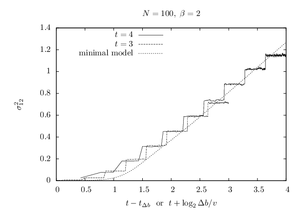
We have to deal with an array whose size grows exponentially with time. It is thus very difficult to pick large values of , and thus also large values of . Indeed, the relevant time scale grows with like , and consequently the minimum number of entries in the array one wants to consider grows like . In practice, we limit ourselves to and . As for the time step , the most convenient is to take it small but finite. We set .
We start with one particle and evolve it for a few hundred units of time using the FIP version of the model. We obtain a traveling wave front, whose tip we eventually label . (The complete front sits in the bins ). From the initial condition built in this way, we evolve all bins for which using the FIP model, and all bins for using the full model. One event in shown in Fig. 3.

Although and are small in this calculation, we see that the regions in impact-parameter space which have similar numbers of dipoles are larger than the local length scale (see Eq. (62)).
After the evolution times and respectively, we measure the position of the front at various impact parameters on a uniform tight grid ranging from to . We use the following definition of the position of the front:
| (66) |
where is the largest for which . Note that in principle, we could have chosen . In practice however, because of the discreteness of in our model, this choice would introduce artefacts which we do not expect in real QCD.
We compute the squared difference of the front positions between the impact parameters and , and average over events. We plot the result as a function of , where is the average front velocity measured at impact parameter .
We compare the results to the correlations obtained in the minimal model, i.e. when we consider two independent realizations of an initial front. We do not attempt to compare to our analytical formulas since the values of that we are able to reach are too small for the approximations that we had to assume to be relevant.
The corresponding plot is displayed in Fig. 4 for , , , and in Fig. 5 with the same parameters except . First, we see that in the full model, the graph of exhibits steps, i.e. is constant by parts. This is related to the hierarchical structure of the model: The correlations between and any of the points at are identical; The same is true for , etc… The logarithmic -scale on the -axis makes the widths of the steps all equal. Next, we see that for small (i.e. impact parameters close to ) there are very little fluctuations in the front positions.
Finally, we see that for , as anticipated, the full model and the minimal ones coincide almost perfectly (Fig. 4). For , i.e. when splittings towards larger dipole sizes are switched on and therefore new correlations appear beyond the ones taken into account in the minimal model, there are some quantitative differences for large (Fig. 5). But we see that using the minimal model instead of the full model that keeps all impact parameters is a good approximation. This corroborates the conclusions of the work in Ref. [18].

4.2 Minimal model
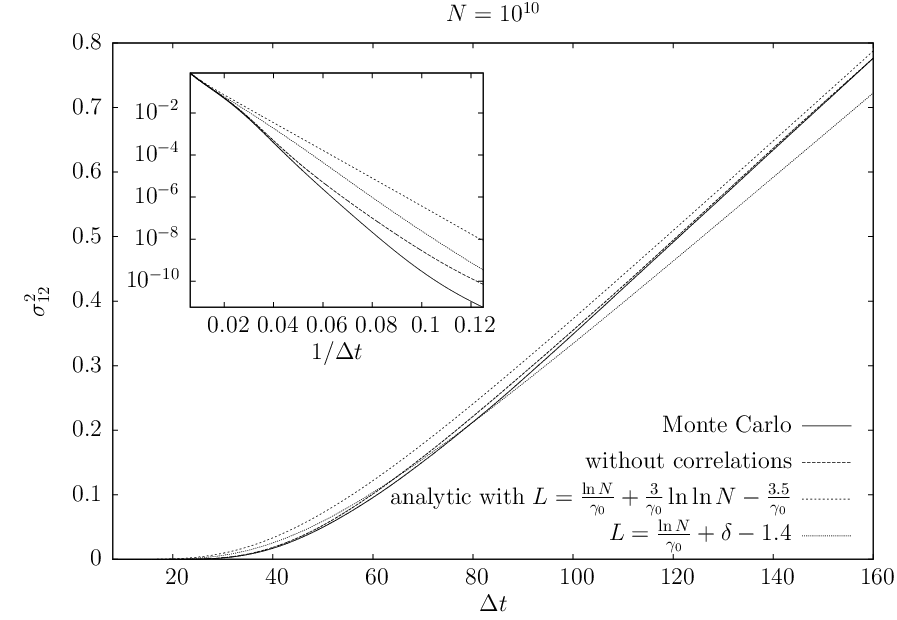
We now set , in which case, as discussed earlier and as checked numerically, the model exactly reduces to a collection of one-dimensional FKPP-like models. Hence, in order to compute two-point correlation functions, it is enough to evolve two realizations of the corresponding FIP model with the constraint that all bins with be identical between the two realizations, and the bins be completely independent. Alternatively, we could also generate one single realization and evolve it for time steps, replicate it at time , and then evolve the two replicas completely independently of each other. The difference between these two possible implementations of the minimal model cannot be accounted for in our analytical calculations, thus the differences that we shall find numerically will give an indication of the model uncertainty. This time, our aim is essentially to check our analytical formulas, thus we will pick very large values of , even if they appear to be unphysical in the QCD context since they would correspond to exponentially small values of the strong coupling constant .
The parameters of the model are obtained from Eq. (8) with , and :
| (67) |
These values are close to , and respectively, which would be the correct parameters if were infinitesimal, in which case (see Eq. (8)).
The numerical results are shown in Fig. 6 for with the two versions of the model (we generated about realizations), and compared with the analytical predictions. We test the two possible choices for the size of the front: Either is a constant, which from our previous experience with FKPP traveling waves [23], we set to
| (68) |
or it is -dependent, namely
| (69) |
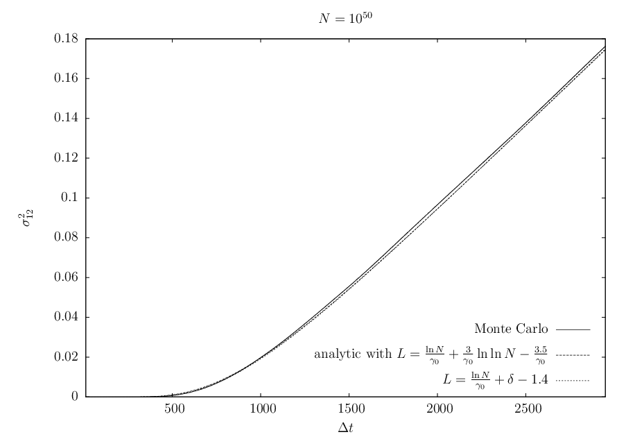
The numerical constants, which are not determined in our theory, were chosen empirically so that they properly describe all numerical data for . In the first case, Eq. (52) is used. In the second case, Eq. (49) is integrated numerically over and . We see that the agreement between the numerical calculation and the analytical predictions is good, except maybe for very small values of where the calculations are not expected to be accurate. Indeed, for the same values of , we also see in Fig. 6 a sizable discreapancy between the two versions of the minimal model. The calculations for are shown in Fig. 7. The numerical results and the theoretical expectations (Eq. (52)) coincide almost perfectly.
Finally, we check that the scaling in Eq. (58) is well reproduced by the numerical data. The Monte-Carlo simulations are shown in Fig. 8, plotted in the appropriate scaling variables. The diffusion constant of a single wave front as well as the velocity are measured from the same data. We see that all curves nicely superimpose for (we show data for values of as large as ), while there are clear deviations for smaller (see the curve for ), as expected.

5 Conclusion
In this paper, we have built a model that possesses the main features of the QCD dipole model including the dynamics in impact-parameter space, and which is furthermore very easy to implement numerically. We have obtained analytical expressions for the fluctuations of the (logarithm of the) saturation scale from one position in impact-parameter space to another one nearby, which gives an indication on the homogeneity of the gluon number density.
Since our analytical calculations are only based on some rather general properties of the model, they should go over to full QCD after appropriate replacement of the parameters, hopefully giving the correct small- (large ) asymptotics.
We have found that the saturation scale varies quite slowly. In the usual notations of QCD, if at position in impact-parameter space the local saturation scale is , then the saturation scale is uniform over a region of size around that position.
Our calculations suffer the usual limitations in this kind of models: Analytical expressions are derived for exponentially large , that is to say, exponentially small values of the strong coupling constant . Although they often may be successfully extrapolated down to (), this is at the cost of tuning constants, and so far, we have not found a systematic procedure to compute finite- corrections.
The next step would probably be a numerical calculation in the case of full QCD, using, as proposed earlier [25], a combination of a Monte Carlo implementation of the color-dipole model in the low-density regime (such an implementation is already available; see Ref. [26, 27, 28] and Ref. [29] for more recent work) and of a numerical solution of the BK equation at the transition to saturation [17]. This looks very challenging, but maybe the nice smoothness of the saturation scale in impact-parameter space that we have found in this paper will help.
Finally, it would be interesting to find an observable which would directly be sensitive to the gluon density at two points in impact-parameter space simultaneously.
Acknowledgments
This work was supported in part by the Department of Energy (USA), and in part by the Agence Nationale pour la Recherche (France), contract ANR-06-JCJC-0084-02.
References
- [1] L. V. Gribov, E. M. Levin and M. G. Ryskin, Phys. Rept. 100, 1 (1983).
- [2] A. H. Mueller and J. W. Qiu, Nucl. Phys. B 268, 427 (1986).
- [3] L. N. Lipatov, Sov. J. Nucl. Phys. 23, 338 (1976); E. A. Kuraev, L. N. Lipatov, and V. S. Fadin, Sov. Phys. JETP 45, 199 (1977); I. I. Balitsky and L. N. Lipatov, Sov. J. Nucl. Phys. 28, 822 (1978).
- [4] I. Balitsky, Nucl. Phys. B 463, 99 (1996).
- [5] Y. V. Kovchegov, Phys. Rev. D 60, 034008 (1999); Phys. Rev. D 61, 074018 (2000).
- [6] J. Jalilian-Marian, A. Kovner, A. Leonidov and H. Weigert, Nucl. Phys. B 504, 415 (1997); Phys. Rev. D 59, 014014 (1999); E. Iancu, A. Leonidov and L. D. McLerran, Phys. Lett. B 510, 133 (2001); Nucl. Phys. A 692, 583 (2001); H. Weigert, Nucl. Phys. A 703 (2002) 823.
- [7] T. Altinoluk, A. Kovner, M. Lublinsky and J. Peressutti, JHEP 0903, 109 (2009).
- [8] For reviews on the FKPP equation and its stochastic extensions, see W. Van Saarloos, Phys. Rep. 386, 29 (2003); D. Panja, Phys. Rep. 393, 87 (2004).
- [9] S. Munier and R. Peschanski, Phys. Rev. Lett. 91, 232001 (2003).
- [10] A. H. Mueller and A. I. Shoshi, Nucl. Phys. B 692, 175 (2004).
- [11] E. Iancu, A. H. Mueller and S. Munier, Phys. Lett. B 606, 342 (2005).
- [12] E. Iancu and D. N. Triantafyllopoulos, Nucl. Phys. A 756, 419 (2005), Phys. Lett. B 610 (2005) 253.
- [13] S. Munier, Phys. Rept. 473, 1 (2009).
- [14] Y. Hatta and A. H. Mueller, Nucl. Phys. A 789, 285 (2007).
- [15] A. H. Mueller, Nucl. Phys. B 415, 373 (1994).
- [16] E. Iancu and L. McLerran, Nucl. Phys. A 793, 96 (2007).
- [17] K. J. Golec-Biernat and A. M. Stasto, Nucl. Phys. B 668, 345 (2003).
- [18] S. Munier, G. P. Salam and G. Soyez, Phys. Rev. D 78, 054009 (2008).
- [19] G. Camici and M. Ciafaloni, Phys. Lett. B 395, 118 (1997).
- [20] K. J. Golec-Biernat, L. Motyka and A. M. Staśto, Phys. Rev. D 65, 074037 (2002).
- [21] A. H. Mueller and D. N. Triantafyllopoulos, Nucl. Phys. B 640, 331 (2002).
- [22] E. Brunet, B. Derrida, Phys. Rev. E 56, 2597 (1997); Comp. Phys. Comm. 121-122 (1999) 376; J. Stat. Phys. 103 (2001) 269.
- [23] E. Brunet, B. Derrida, A. H. Mueller and S. Munier, Phys. Rev. E 73, 056126 (2006).
- [24] M. Abramowitz and I. A. Stegun, Handbook of Mathematical Functions, (1964) Dover Publications, New York. ISBN 0-486-61272-4.
- [25] S. Munier, Phys. Rev. D 75, 034009 (2007).
- [26] G. P. Salam, Nucl. Phys. B 461, 512 (1996).
- [27] G. P. Salam, Comput. Phys. Commun. 105, 62 (1997).
- [28] A. H. Mueller and G. P. Salam, Nucl. Phys. B 475, 293 (1996).
- [29] E. Avsar, G. Gustafson and L. Lonnblad, JHEP 0507 (2005) 062; JHEP 0701 (2007) 012.