Error estimation and reduction with cross correlations
Abstract
Besides the well-known effect of autocorrelations in time series of Monte Carlo simulation data resulting from the underlying Markov process, using the same data pool for computing various estimates entails additional cross correlations. This effect, if not properly taken into account, leads to systematically wrong error estimates for combined quantities. Using a straightforward recipe of data analysis employing the jackknife or similar resampling techniques, such problems can be avoided. In addition, a covariance analysis allows for the formulation of optimal estimators with often significantly reduced variance as compared to more conventional averages.
pacs
05.10.Ln, 05.70.Fh, 64.60.F-I Introduction
Monte Carlo simulations, and in particular Markov chain based methods, have matured over the last decades into a highly versatile and powerful toolbox for studies of systems in statistical and condensed-matter physics [1, 2], ranging from classical spin models [3] over soft-matter problems [4] to quantum systems [5]. Their competitiveness with other approaches such as, e.g., field-theoretic expansions for the study of critical phenomena [6, 7], is largely based on the development and refinement of a number of advanced simulation techniques such as cluster algorithms [8] and generalized-ensemble methods [9, 10].
Equally important to the generation of simulation data, however, is their correct and optimal analysis. In this field, a number of important advances over the techniques used in the early days have been achieved as well. These include, e.g., the finite-size scaling (FSS) approach [11], turning the limitation of simulational methods to finite system sizes into a systematic tool for accessing the thermodynamic limit, reweighting techniques [12], lifting the limitation of numerical techniques to the study of single points in parameter space to allow for continuous functions of estimates to be studied, as well as advanced statistical tools such as the jackknife and other resampling schemes of data analysis [13].
Of these techniques, the statistical data analysis appears to have received the least attention. Hence, while FSS analyses, even including correction terms, are quite standard in computer simulation studies [1], a proper analysis and reduction of statistical errors and bias appears to be much less common. Here, resampling methods turn out to be very valuable. Although such techniques offer a number of benefits over more traditional approaches of error estimation, their adoption by practitioners in the field of computer simulations has not yet been as universal as desirable. It is our understanding that this is, in part, due to a certain lack in broadly accessible presentations of the basic ideas which are, in fact, very simple and easy to implement in computer codes, as is demonstrated below.
More specifically, data generated by a Monte Carlo (MC) simulation are subject to two types of correlation phenomena, namely (a) autocorrelations or temporal correlations for the case of Markov chain MC (MCMC) simulations, which are directly related to the Markovian nature of the underlying stochastic process and lead to an effective reduction of the number of independently sampled events and (b) cross correlations between different estimates extracted from the same set of original time series coming about by the origin of estimates in the same statistical data pool. The former can be most conveniently taken into account by a determination of the relevant autocorrelation times and a blocking or binning transformation resulting in an effectively uncorrelated auxiliary time series [14]. Such analyses are by now standard at least in seriously conducted simulational studies. On the contrary, the effects of cross correlations have been mostly neglected to date (see, however, Refs. [15, 16, 17, 18]), but are only systematically being discussed following our recent suggestion [19, 20]. In this article, we show how such cross correlations lead to systematically wrong estimates of statistical errors of averaged or otherwise combined quantities when a naïve analysis is employed, and how a statistically correct analysis can be easily achieved within the framework of the jackknife method. Furthermore, one can even take benefit from the presence of such correlation effects for significantly reducing the variance of estimates without substantial additional effort. We demonstrate the practical relevance of these considerations for a finite-size scaling study of the Ising model in two and three dimensions.
The rest of this article is organized as follows. In Sec. II we give a general recipe for a failsafe way of Monte Carlo data analysis, taking into account the effects of autocorrelations and cross correlations mentioned above. After discussing the complications for the more conventional analysis schemes (but not the jackknife method) introduced by histogram reweighting and generalized-ensemble simulation techniques in Sec. III, we outline the role of cross correlations in the process of averaging over a set of MC estimates in Sec. IV and discuss the choice of an optimal averaging procedure. In Sec. V, these ideas are applied to a simulational study of the critical points of the two- and three-dimensional Ising models. Finally, Sec. VI contains our conclusions.
II Monte Carlo error analysis
Compared to the task of estimating the uncertainty in the result of a lab experiment by simply repeating it several times, there are a number of complications in correctly determining — and possibly even reducing — statistical fluctuations in parameter estimates extracted from MCMC simulations. Firstly, due to the memory of the Markovian process, subsequent measurements in the time series are correlated, such that the fluctuations generically appear smaller than they are. This issue can be resolved by a blocking of the original time-series data. Secondly, one often needs to know the precision of parameter estimates which are complicated (and sometimes non-parametric) functions of the measured observables. Such problems are readily solved using resampling techniques such as the jackknife.
II.1 Autocorrelations
Consider a general Monte Carlo simulation with the possible values of a given observable appearing according to a probability distribution . This form, of course, implies that the system is in thermal equilibrium, i.e., that the underlying stochastic process is stationary. The probability density could be identical to the Boltzmann distribution of equilibrium thermodynamics as for the importance-sampling technique [21], but different situations are conceivable as well, see the discussion in Sec. III below. If we assume ergodicity of the chain, the average
for a time series of measurements is an unbiased estimator of the mean
In contrast to , the estimator is a random number, which only coincides with in the limit . Under these circumstances, simulational results are only meaningful if in addition to the average we can also present an estimate of its variance . Note that, although the distribution of individual measurements might be arbitrary, by virtue of the central limit theorem the distribution of the averages must become Gaussian for . Hence, the variance is the (only) relevant parameter describing the fluctuations of . If subsequent measurements , , are uncorrelated, we have
| (1) |
which can be estimated without bias from [22]
| (2) |
i.e., . This is what we do when estimating the statistical fluctuations from a series of independent lab experiments. Markov chain simulations entail the presence of temporal correlations, however, such that the connected autocorrelation function,
| (3) |
is non-zero in general (see, e.g., Ref. [23]). Stationarity of the chain implies that . Then, the variance of becomes
| (4) |
Monte Carlo correlations decline exponentially, i.e.,
| (5) |
to leading order, defining the exponential autocorrelation time . Due to this exponential decay, for the deviations of the factors of Eq. (4) from unity can be neglected [24], and defining the integrated autocorrelation time as
| (6) |
one has
| (7) |
In view of the reduction of variance of the average relative to a single measurement in Eq. (1), Eq. (7) states that the effective number of independent measurements in the presence of autocorrelations is reduced by a factor of . The autocorrelation times and are not identical, but one can show that the latter is a lower bound of the former, [25].

As long as the autocorrelation time is finite, the distribution of averages still becomes Gaussian asymptotically, such that for the variance remains the relevant quantity describing fluctuations. To practically determine from Eq. (4), an estimate for the autocorrelation function is required. This can be found from the definition (3) by replacing expectation values with time averages. It turns out, however, than upon summing over the contributions of the autocorrelation function for different time lags in Eq. (4) divergent fluctuations are incurred, enforcing the introduction of a cut-off time [26, 27]. Several approximation schemes have been developed using such estimators, but they turn out to have severe drawbacks in being computationally expensive, hard to automatize and in that estimating their statistical accuracy is tedious (see Ref. [14]).
A more efficient and very intuitive technique for dealing with autocorrelations results from a blocking transformation in the spirit of the renormalization group [14] (in fact, this idea was already formulated by Wilson [28]). Much like block spins are defined there, one combines adjacent entries of the time series,
| (8) |
and defines block averages
| (9) |
cf. Fig. 1(a). This procedure results in a shorter effective time series with entries. (We assume for simplicity that is an integer multiple of .) Obviously, the average and its variance are invariant under this transformation. Under the exponential decay (5) of autocorrelations of the original series it is clear (and can be shown explicitly [14]), however, that subsequent block averages , are less correlated than the original measurements and . Furthermore, the remaining correlations must shrink as the block length is increased, such that asymptotically for (while still ensuring ) an uncorrelated time series is produced. Consequently, the naïve estimator (2) can be legally used in this limit to determine the variance of the average. For the finite time series encountered in practice, a block length and must be used. This is illustrated in Figure 2 showing the estimate (2) for a blocked time series with autocorrelation time as a function of the block length . It approaches the true variance from below, eventually reaching a plateau value where any remaining pre-asymptotic deviations become negligible compared to statistical fluctuations. If the available time series is long enough (as compared to ), it is often sufficient to simply lump the data into as few as some hundred blocks and restrict the subsequent data analysis to those blocks. As a rule of thumb, in practical applications it turns out that a time series of length is required for a reliable determination of statistical errors as well as autocorrelation times. From Eqs. (2) and (6) it follows that the integrated autocorrelation time can be estimated from
| (10) |
within this scheme, where needs to be chosen in the plateau regime of Fig. 2.

II.2 Covariance and bias
Apart from providing an estimate of for simple quantities, the blocking procedure has the advantage of resulting in an effectively uncorrelated auxiliary time series which can then be fed into further statistical machinery, much of which is restricted to the case of independent variables. Resampling schemes such as the jackknife [13] provide error and bias estimates also for non-linear functions of observables without entailing truncation error or requiring assumptions about the underlying probability distributions.
While can be directly computed from the blocked time series of via the estimator (2), this approach fails for non-linear functions of expectation values , , such as, e.g., susceptibilities or cumulants. A standard approach for such cases is the use of error propagation formulas based on Taylor expansions [22],
| (11) |
Apart from the truncation error resulting from the restriction to first order in the expansion, this entails a number of further problems: if the averages , etc. are correlated due to their origin in the same simulation, cross-correlation terms need to be included as well. Even worse, for the case of non-parametric parameter estimates, such as determining the maximum of some quantity by reweighting (see below) or extracting a critical exponent with a fitting procedure, error propagation cannot be easily used at all.
Such problems are avoided by methods based on repeated sampling from the original data pool, using the properties of these meta samples to estimate (co-)variance, reduce bias etc. These are modern techniques of mathematical statistics whose application only became feasible with the general availability of computers [13]. Most straightforwardly applicable is the jackknife procedure, where the meta samples consist of all of the original time series apart from one data block, cf. Fig. 1(b). Assume that a set of simulations resulted in a collection of time series , , , for different observables, system sizes, temperatures etc. Applying the blocking procedure described above, it is straightforward to divide the series in effectively uncorrelated blocks. It is often convenient to use the same number of blocks for all series (e.g., 100) which can easily be arranged for by the blocking transformation as long as is larger than some minimum value (e.g., ) for each simulation and observable. If then denotes the block over all series according to Eq. (8), where for a constant number of blocks the block lengths might vary between the different series under consideration, one defines the corresponding jackknife block as the complement
| (12) |
cf. Fig. 1. Considering now an estimator for some parameter depending on (some or all of) the different series, we define the corresponding estimates restricted to jackknife block ,
| (13) |
The variation between these estimates taken from the same original data can be used to infer the sample variance. If one denotes the average of the jackknife block estimators (13) as
| (14) |
an estimate for the sample variance of the estimator is given by [29]
| (15) |
This is very similar to the simple estimate (2) for the variance of the average, but it comes with a different prefactor which serves a twofold purpose: it reweights the result from the effective jackknife series of length to the original length and takes care of the fact that all of the jackknife block estimates are strongly correlated due to them being based on (almost) the same data. The general Eq. (15) forms a conservative and at most weakly biased estimate of the true variance [13], which lacks the truncation error of schemes based on Eq. (11) and is applicable to non-parametric parameter estimates.
In a slight generalization of Eq. (15) it is possible to also estimate covariances. For a number of estimators , , , , a robust jackknife estimator of the covariance matrix is given by
| (16) |
In a similar way the bias of estimators can be reduced, i.e., deviations between the mean of an observable and the expectation value of some estimator that disappear with increasing sample length. For a detailed discussion we refer the reader to Refs. [29, 13].
A general procedure for the analysis of simulation data based on blocking and jackknife techniques hence has the following form:
- 1.
Decide on the number of jackknife blocks to be used. For most purposes, of the order of blocks are sufficient.
- 2.
For each original time series recorded in a collection of simulations, examine the block averages (9) as a function of the block length . If the result for blocks is in the plateau regime of Fig. 2 everything is fine; otherwise, one needs to record a longer time series (and possibly take measurements less frequently to keep the amount of data manageable).
- 3.
III Histograms and errors
An increasing number of successful Monte Carlo techniques rely on reweighting and the use of histograms [1]. This includes the (multi-)histogram method of Refs. [12, 30] as well as the plethora of generalized ensemble techniques ranging from multicanonical simulations [9] to Wang-Landau sampling [10]. Such methods are based on the fact that samples taken from a known probability distribution can always be translated into samples from another distribution over the same state space. Assume, for simplicity, that states are labeled as appropriate for a spin system. If a sequence , , , was sampled from a stationary simulation with probability density , an estimator for the expectation value of the observable relative to the equilibrium distribution is given by
| (17) |
For a finite simulation this works as long as the sampled and the equilibrium distributions have sufficient overlap, such that the sampled configurations can be representative of the equilibrium average at hand. For simple sampling one has and hence must weight the resulting time series with the Boltzmann factor
| (18) |
where denotes the energy of the configuration and is the partition function at inverse temperature . For importance sampling, on the other hand, , such that averages of time series are direct estimates of thermal expectation values. If samples from an importance sampling simulation with should be used to estimate parameters of , Eq. (17) yields the familiar (temperature) reweighting relation
| (19) |
where . Completely analogous equations can be written down, of course, for reweighting in parameters other than temperature. Similarly, canonical averages at inverse temperature are recovered from multicanonical simulations via using Eq. (17) with and .
Reliable error estimation (as well as bias reduction, covariance estimates etc.) for reweighted quantities is rather tedious with traditional statistical techniques such as error propagation [31]. Resampling methods, on the other hand, allow for a very straightforward and reliable way of tackling such problems 11 1 Note that when using the Wang-Landau method as a direct estimate of the density of states to be used for computing thermal expectation values, due to the non-Markovian nature of the algorithm there is currently no known approach of reliably estimating the present statistical fluctuations apart from repeating the whole calculation a certain number of times.. For the jackknife approach, for instance, one computes jackknife block estimates of the type (17) by simply restricting the set of time series to the jackknife block . With the jackknife average (14), e.g., the variance estimate (15) with can be straightforwardly computed. Similar considerations apply to covariance estimates or bias reduced estimators [13]. Extremal values of thermal averages can be determined to high precision from the continuous family of estimates (19), where error estimates again follow straightforwardly from the jackknife prescription.
IV Variance reduction
Temporal correlations resulting from the Markovian nature of the sampling process have been discussed in Sec. II.1 above, and we assume that they have been effectively eliminated by an appropriate binning procedure. Extracting a number of different parameter estimates , , , from the same number of original simulations it is clear, however, that also significant cross correlations between estimates and can occur. These have profound consequences for estimating statistical error and reducing it by making the best use of the available data [19].
If a given parameter estimate depends on several observables of the underlying time series that exhibit cross correlations, this fact is automatically taken into account correctly by the jackknife error estimate (15). This is in contrast to error analysis schemes based on error propagation formulae of the type (11), where any cross correlations must be taken into account explicitly. Insofar the outlined approach of data analysis is failsafe. We want to go beyond that, however, in trying to optimize statistical precision of estimates from the available data. If we attempt to estimate a parameter , we ought to construct an estimator
which is a function of the underlying time series with the property that (at least for ). Obviously, there usually will be a large number of such functions and it is not possible, in general, to find the estimator of minimal variance. We therefore concentrate on the tractable case where is a linear combination of other estimators , ,
| (20) |
There are different possibilities to ensure the condition :
- 1.
All estimators have the same expectation, , and .
- 2.
One estimator is singled out, say , , and the rest has vanishing expectation, , arbitrary, .
- 3.
More complicated situations.
The first type describes the case that we have several different estimators for the same quantity and want to take an average of minimum variance [19]. The second case is tailored for situations where existing symmetries allow to construct estimators with vanishing expectation whose cross correlations might reduce variance [20].
To optimize the analysis, the parameters in (20) should be chosen such as to minimize the variance
| (21) |
For case one above, we introduce a Lagrange multiplier to enforce the constraint , and the optimal choice of is readily obtained as
| (22) |
leading to a minimum variance of
| (23) |
Very similarly, case two leads to the choice 22 2 Note that Eqs. (4) and (5) of Ref. [20] contain some mistakes, but Eq. (7) and the implementation (24) are correct.
| (24) |
where denotes the submatrix of with . Since the formalism for both cases is practically identical, in the following we will concentrate on case one.
Let us take the time to compare the optimal choice of weights expressed in Eqs. (22) and (24) with that used in more traditional approaches. Ignoring the presence of cross correlations, several parameter estimates are often combined using an error weighting scheme only, i.e., by choosing weights
| (25) |
While the more general expression (22) reduces to the weights (25) in the absence of correlations, the choice (25) is not optimal as soon as cross correlations are present. Still, the resulting average remains a valid estimator of the parameter . In contrast, the usually used variance estimate derived from the expression
| (26) |
is no longer even correct when cross correlations come into play. As will be seen below from the discussion of Ising model simulations in Sec. V, generically leads to underestimation of the true variance, but occasionally over-estimates are possible as well.
The practical implementation of the described scheme of weighting and error analysis is straightforward with the toolset outlined in the previous sections. The covariance matrix of the estimates is readily computed via the jackknife expression (16). This allows to estimate the optimal weights from inserting in Eq. (22) (or the analogue (24) for case two) and the variance of the resulting optimal estimator is determined from the expression (23). In total, the necessary analysis can be summarized as follows:
- 1.
Perform a binning analysis to see whether for a given number of blocks the block averages (9) for all time series at hand are effectively uncorrelated.
- 2.
- 3.
In some cases, it is necessary to already have variance estimates of intermediate data available for properly determining the jackknife block estimates . This typically occurs when is a parameter resulting from an (ideally error weighted) fit to a number of data points, such as for the case of a critical exponent, see the discussion below in Sec. V. In these cases it is straightforward to iterate the jackknifing procedure to second order by considering each jackknife block as the initial time series of another jackknife analysis [32].
V Application to the Ising model

Although the outlined scheme of Monte Carlo data analysis is completely general, it is useful to see how it works out for a specific example. In particular, one would like to know if the typical cross correlations are sufficiently strong to have significant impact on the results. To answer this question, we performed a finite-size scaling (FSS) analysis of the ordering transition of the ferromagnetic Ising model in two and three dimensions.
V.1 Simulation details
We studied the critical behavior of the nearest-neighbor, zero-field, ferromagnetic Ising model with Hamiltonian
| (27) |
on square and simple cubic lattices of edge length , using periodic boundary conditions. Close to criticality, an importance-sampling Monte Carlo simulation with local update rule suffers from critical slowing down, , with a dynamical critical exponent . To alleviate this problem, we used the single-cluster update algorithm [33] resulting in a dramatic speed-up of the relaxation process. For two and three dimensions we performed simulations at a fixed temperature close to the asymptotic critical temperature for a number of different system sizes to enable a systematic FSS study. The raw data consisted of time series with approximately independent samples of the configurational energy and magnetization for each system size under consideration. Using the jackknifing analysis described above, these original time series were then analyzed using effectively uncorrelated bins, where was chosen unless stated otherwise.
| fits | correlation coefficients/weights | ||||||||||||
|---|---|---|---|---|---|---|---|---|---|---|---|---|---|
| d.o.f. | |||||||||||||
| 32 | 192 | % | 4 | ||||||||||
| 32 | 192 | % | 4 | ||||||||||
| 32 | 192 | % | 4 | ||||||||||
| 32 | 192 | % | 4 | ||||||||||
| 32 | 192 | % | 4 | ||||||||||
| % | |||||||||||||
| % | |||||||||||||
| % | 11 1 Note that the similar Table II of Ref. [19] contains a mistake in the last two lines, where the weights and as well as and appear interchanged with respect to the correct data represented here. | ||||||||||||
| % | |||||||||||||
| % | |||||||||||||
V.2 Finite-size scaling analysis
There is now a broad consensus that finite-size effects are (in most cases) not merely a drawback of approaches depending on finite system sizes, but can be turned into a powerful tool for extracting the asymptotic behavior [11]. A number of different practical implementations of this idea in terms of specific FSS schemes have been derived and successfully applied to the analysis of critical phenomena, see, e.g., Refs. [34, 35, 36]. Although our considerations regarding the data analysis apply rather generally to all these techniques, for illustrative purposes we concentrate here on the rather popular method outlined in Ref. [34]. It is focused on the analysis of the locations and values of extrema of standard thermodynamic quantities such as the specific heat, magnetic susceptibility, cumulants etc. According to the theory of finite-size scaling [11, 37], the locations of such pseudo-critical points are shifted away from the true critical coupling according to
| (28) |
where denotes an observable with a pseudo-critical maximum such as the specific heat (for ). The generic value for the shift exponent predicted by FSS theory is , where is the correlation length exponent (for exceptions see, e.g., Ref. [38]). A drawback of using Eq. (28) directly is that non-linear fits in the three parameters , and resp. are required even for the simplest case of ignoring the correction-to-scaling terms in brackets. To alleviate this problem, it has been suggested to consider quantities such as the magnetization cumulants [39]
| (29) |
for which the maxima of the temperature derivatives have a critical scaling form
| (30) |
and hence allow to determine without prior knowledge of the transition coupling . If, again, the correction terms in brackets are ignored, this form even represents a linear fit (in logarithmic representation) resulting in very stable results. While initially only the fourth-order cumulant was considered, the authors of Ref. [34] suggested to use a variety of different cumulants with , , , to improve the accuracy of the estimate. A number of further quantities with the same scaling behavior can be constructed, for instance logarithmic temperature derivatives of the magnetization,
| (31) |
which for , , yields another series of estimates.
Once has been determined from fits of the functional forms (30) and (31) to the data, one might return to the shift relation (28) and (assuming ) determine the transition coupling from linear fits with a fixed value of . Finally, the remaining standard critical exponents can be estimated from the well-known FSS forms of the specific heat , the magnetization and the magnetic susceptibility ,
| (32) |
where denotes the (modulus of the) magnetization at its inflection point. The directly estimated exponents are therefore and the FSS exponents , and , which can be combined to yield , , and . The remaining exponents and are not directly determined here; instead we assume that their values are deduced from the exponents , , and via standard scaling relations.
| fits | correlation coefficients/weights | ||||||||||||
|---|---|---|---|---|---|---|---|---|---|---|---|---|---|
| % | |||||||||||||
| % | |||||||||||||
| % | |||||||||||||
| % | |||||||||||||
| % | |||||||||||||
| % | |||||||||||||
| % | |||||||||||||
| % | |||||||||||||
| % | |||||||||||||
| % | |||||||||||||
| % | |||||||||||||
| % | |||||||||||||
| % | |||||||||||||
For determining the (location and value of the) maxima occurring in Eqs. (28), (30), (31) and (32), we used the reweighting technique outlined in Sec. III starting from the data of a single simulation per system size performed at or close to the asymptotic transition point. The derivatives with respect to in Eqs. (30) and (31) are easily shown to be equivalent to combinations of moments of energy and magnetization at a single, fixed temperature [34]. For the fourth-order cumulant , for instance, one has
| (33) |
Therefore no numerical differentiation is required when making use of the relations (30) and (31). In some situations it might be impractical to store the whole time series of original measurements of internal energy and magnetization, in which case the exact reweighting relation (19) might be replaced by a Taylor expansion with respect to around the simulation coupling , where then cumulants of and appear as the expansion coefficients. In most cases, however, it is much simpler and more versatile in terms of the data analysis to work with the original time series. In view of the typically available storage resources today, this approach should be comfortably feasible in most situations.
Considering the set of critical exponents , , , (as well as and ), it is useful to recall that they are subject to a number of exact scaling relations, namely the Rushbrooke identity , Fisher’s scaling law , the relation , as well as (in most cases) the hyperscaling relation , where is the spatial dimension [40]. As a consequence of these four equations, only two of the six original exponents are independent. While the scaling relations have been occasionally used to check a set of independently estimated exponents for consistency, we would like to point out that the existence of these exact relations should rather be used for improving the precision of exponent estimates. In particular, in the language of the renormalization group, it is natural to express the conventional scaling exponents in terms of the scaling dimensions and of the operators coupling to temperature and magnetic field [41], respectively, which are the only relevant operators for the Ising model [42]. For the four exponents considered here, this means that
| (34) |
such that can be independently estimated from and , whereas might be determined from as well as .
V.3 Two-dimensional Ising model
For the two-dimensional (2D) Ising model, single-cluster update simulations were performed for square lattices of size , , , , , , and . All simulations were done directly at the asymptotic critical coupling . For the range of system sizes under consideration, it turned out that simulations at this single temperature were sufficient for reliably studying the pseudo-critical points defined by the maxima of the various quantities under consideration by reweighting, i.e., the overlap of histograms between the simulation and analysis temperatures turned out to be sufficiently large.
We first extracted a number of estimates of the correlation length exponent from investigating the maxima of logarithmic derivatives of magnetization moments for , and as well as the maxima of the derivatives of the second-order and fourth-order cumulants and using the reweighting scheme outlined above. The locations and values of the maxima themselves were determined by a golden section search algorithm [43]. The resulting maxima as a function of system size are shown in Fig. 3 together with fits of the forms (30) and (31) to the data. Here, we used fits without the correction terms in the brackets of Eqs. (30) and (31) on the fit range , which works very well as is apparent from the presentation in Fig. 3 and the corresponding values of the quality-of-fit parameter [22] listed in the eighth column of Table 1. The fourth and fifth column contain the resulting estimates of the exponent together with the statistical errors estimated from a weighted least-squares fitting procedure [43]. A glance at Table 1 reveals that all single estimates are statistically consistent with the exact result , but they exhibit a rather large variation in statistical accuracy with the biggest statistical error being almost three times larger than the smallest. We use the jackknife estimator (16) and a second-order jackknifing procedure to estimate the statistical correlations of the individual estimates of . The data on the right hand side of Table 1 showing the correlation coefficients for the different estimates reveal that correlations between all pairs of estimates are large with . With all estimates being derived from similar expressions containing magnetic moments, this result probably does not come as a surprise.
| exact |
|---|
Under these circumstances, one might wonder whether it is worthwhile to attempt a linear combination of the form (20) of the various estimates rather than quoting the single most precise estimate as final result, which in the present case is given by the value resulting from the FSS of . For the purpose of combining estimates, we consider the traditional approaches of taking a plain average with
| (35) |
as well as the error-weighted average of Eq. (25) and compare them to the truly optimal covariance-weighted average defined by the weights of Eq. (22). Ignoring the presence of correlations (as was the case in most previous studies), one would estimate the error associated to the plain average as
| (36) |
and, likewise, the variance of the error-weighted average is given by as defined in Eq. (26). The true variances of and in the presence of correlations, on the other hand, can also be easily derived formally, and will contain the elements of the covariance matrix of the individual estimates . From the practical perspective, the jackknifing analysis outlined here automatically takes those correlations into account. We refer to these correctly defined variances with the notation .
The plain, error-weighted and covariance-weighted averages for with the corresponding variance estimates are listed in the lower part of columns four and five of Table 1. As with the individual estimates, each of the three averages is statistically compatible with the exact result . While the naïve error estimates seem to indicate that performing the plain or error-weighted average reduces statistical fluctuations compared to the single estimates, taking correlations into account with the jackknifing scheme resulting in reveals that variances are grossly underestimated by and, in fact, compared to both the plain () and error-weighted () averages the single estimate of stemming from has smaller statistical fluctuations (). Performing those averages therefore decreases precision instead of improving it! The truly optimal average of Eq. (22), on the other hand, results in the estimate , whose fluctuation is about 2–3 times smaller than those of the error-weighted average and the single most precise estimate. The reduced variance of this last estimate seems to be corroborated by the smallest deviation also from the exact result . A glance at the data collected in Table 1 reveals that, somewhat astonishingly, the optimal average is smaller than all of the individual estimates of (see also the graphical representation of this fact in Fig. 1 of Ref. [19]). This situation which, of course, can never occur for the error-weighted average where all weights , is connected to the fact that the more general weights of Eq. (22) are unbounded and, in particular, can become negative. This fact reflects in the computed weights for the different averaging schemes collected in the lower right hand part of Table 1. Clearly, the weights for the error-weighted and covariance-weighted averages are dramatically different and, in particular, some of the latter turn out to be negative. It is intuitively clear that such negative weights are necessary to cancel the effects of strong mutual correlations. The asymmetry in the weights leading to the possibility of the average lying outside of the range of the individual estimates results from the asymmetry of the individual variances in connection with the cross correlations. This effect can be explicitly understood for the case of only two estimates, cf. the discussion in Appendix A.
One might wonder whether the suggested weighting scheme requiring to estimate the full covariance matrix is statistically robust. It is clear, for instance, that the jackknife estimator (16) for the covariance will become more precise as more jackknife blocks are used — at the expense of an increased computational effort. To check for such effects we repeated our analysis while using instead of jackknife blocks. Most of the estimates for the correlation coefficients are almost unchanged by this new analysis with the largest deviation being of the order of 3%. The same holds true for the resulting weights in the optimal average, where only the weight of the estimate resulting from changes substantially from to . The final optimal estimate is fully compatible statistically with the analysis using jackknife blocks. Using (as a consistency check) completely independent simulations for producing the individual estimates of , on the other hand, indeed results in a unit matrix of correlation coefficients within statistical errors and, consequently, the error-weighted and covariance-weighted averages coincide in this limit. Finally, we also find that the numerical inversion of the covariance matrix required for computing the weights in Eq. (22) is in general stable and unproblematic. It is clear, however, that in the presence of very strong correlations the resulting weights of individual estimates will depend sensitively on the entries of the covariance matrix, since in the limit of perfect correlations all choices of weights become degenerate, see also the discussion of the case of only two estimates in Appendix A.
We now turn to the determination of the transition coupling from the shift relation (28). We considered the locations of the extrema of the specific heat , the slope of the (modulus of the) magnetization, the logarithmic derivatives for , and , the cumulant derivatives and as well as the magnetic susceptibility . In order to most clearly demonstrate the effects of the present correlations, we first performed fits of the form (28) using the exact correlation length exponent . The corresponding fit results are collected in Table 2. For the fits we ignored the correction terms indicated in the brackets of Eq. (28), leaving out the smallest system sizes instead. This approach appears justified in view of the good fit qualities reflected in the values of Table 2. As for the fits for determining , all single estimates of are consistent with the true asymptotic values of within error bars. The corresponding standard deviations, however, vary dramatically, decreasing by a factor of from the estimate resulting from to that of the susceptibility . The results of the correlation analysis are presented on the right-hand side of Table 2: while the logarithmic magnetization derivatives and cumulants again show very strong correlations, the results of the remaining quantities are somewhat more independent, showing, in particular, a rather clear separation of the energetic from the magnetic sector. For the averages of single estimates the present correlations again lead to a significant underestimation of the true variance for the plain and error-weighted cases and, in fact, both of them are less precise than the best single estimate stemming from the scaling of the susceptibility , cf. the data in the lower part of Table 2. The truly optimal average of Eq. (22) results in , where the statistical error is about threefold reduced compared to the error-weighting scheme. Very similar results are found when using the value found from the analysis summarized in Table 1, where we arrive at a final covariance-weighted average of . Here, the second error estimate in square brackets refers to the sensitivity of the result for to the uncertainty in indicated above, which turns out to be symmetric with respect to upwards and downwards deviations of here.
As an alternative to the two-step process of first determining from the relations (30) and (31) and only afterwards estimating from Eq. (28), one might consider direct fits of the form (28) to the maxima data of the 8 observables listed above determining and in one go. Here, again, fits on the range neglecting any corrections to the leading scaling behavior are found to be sufficient. The results for the plain, error-weighted and covariance-weighted averages for both parameters, and , are collected in Table 3. Consistent with the previous results, it is seen that neglecting correlations in error estimation leads to a sizable underestimation of errors and, on the other hand, using the optimal weighting scheme of Eq. (22) statistical errors are significantly reduced, an effect which is also nicely illustrated by the very good fit of the resulting parameter estimates with the exact values.
| exact |
|---|
| fits | correlation coefficients/weights | ||||||||||||
|---|---|---|---|---|---|---|---|---|---|---|---|---|---|
| d.o.f. | |||||||||||||
| 8 | 128 | % | 5 | ||||||||||
| 8 | 128 | % | 5 | ||||||||||
| 8 | 128 | % | 5 | ||||||||||
| 32 | 128 | % | 3 | ||||||||||
| 32 | 128 | % | 3 | ||||||||||
| % | |||||||||||||
| % | |||||||||||||
| % | |||||||||||||
| % | |||||||||||||
| % | |||||||||||||
Finally, we turn to the determination of the remaining critical exponents. As outlined above, we do this by combining different estimates using covariance analysis to improve the results for the scaling dimensions, thus ensuring that the scaling relations are fulfilled exactly. From a glance at Eq. (34) one reads off that the magnetic scaling dimension can be determined from and . We therefore determine from the FSS of the (modulus of the) magnetization at its inflection point and estimate from the FSS of the susceptibility maxima, resulting in and , respectively. As the correlation analysis reveals, the two resulting estimates of are anti-correlated to a considerable degree with correlation coefficient . As a consequence, conventional error analysis neglecting correlations over-estimates statistical fluctuations. Still, choosing optimal weights according to Eq. (22) is able to reduce variance, resulting in a combined estimate right on top of the exact result , cf. the data collected in Table 4. The energetic scaling dimension , on the other hand, might be computed from as well as . We therefore use the five individual estimates of listed in Table 1 as well as the FSS of the maximum of the specific heat to estimate . The latter fits are somewhat problematic due to the logarithmic singularity of the specific heat corresponding to , and it turns out that a fit of the form
including a scaling correction is necessary to describe the data. Combining all individual estimates in an optimal way, we arrive at , well in agreement with the exact result , cf. the right hand side of Table 4.
V.4 Three-dimensional Ising model
Cluster-update simulations of the ferromagnetic Ising model in three dimensions (3D) were performed for simple-cubic lattices of edge lengths , , , , , , , and . All simulations were performed at the coupling reported in a high-precision study as estimate for the transition point [45], since it turned out that the maxima of the various quantities under consideration were all within the reweighting range of this chosen simulation point for the system sizes and lengths of time series at hand.
For determining the correlation-length exponent we again considered the scaling of the logarithmic magnetization derivatives for , and and the derivatices of the cumulants and . We find scaling corrections to be somewhat more pronounced than for the two-dimensional model for the system sizes studied here. For the logarithmic magnetization derivatives we therefore performed fits of the form (31) including the correction term on the full range , where the resulting values of the effective correction exponent were (), () and (), respectively. For the cumulants and , on the other hand, corrections were too small to be fitted reliably with our data, such that they were effectively taken into account by dropping the small lattice sizes instead, while using fits of the form (30) with fixed. The corresponding fit data are collected in Table 5. The estimated standard deviations of the individual estimates are again found to be very heterogeneous, but the correlations between the different estimates are somewhat smaller than in two dimensions, in particular between the magnetization derivatives and the cumulants, cf. Table 5. Comparing to the case of fits without corrections, it is seen that this latter effect is partially due to the use of two different fit forms for the two types of quantities. (The fits for and also include a reduced range of lattice sizes which could lead to a decorrelation, but this effect is found to be much less important than the difference in the fit forms.) Considering the averages of individual estimates, as a result of these smaller correlations the underestimation of statistical errors in the naïve approach as well as the reduction of variance through the optimized estimator (22) is somewhat less dramatic than for the two-dimensional model, but the qualitative behavior appears to be very much the same. As our final estimate we quote , very well in agreement with the reference value taken from a survey of recent literature estimates compiled in Ref. [44].
In a second step we determined the transition coupling from fits of the functional form (28) to the maxima of the quantities listed in Table 2. As for the fits, however, the inclusion of an effective correction term as indicated in Eq. (28) turned out to be necessary for a faithful description of the scaling data. The plain, error-weighted and covariance-weighted averages of the corresponding estimates are listed in the first two data columns of Table 6 together with their standard deviations, the results being consistent with the reference value. We also tried non-linear three-parameter fits of the form (28) to the data, determining and simultaneously. For this case, the precision of the data is not high enough to reliably include corrections to scaling. Still, the improved results are well consistent with the reference values of Refs. [45, 44], cf. the middle columns of Table 6.
| Eq. (28), | Eq. (28) | Eq. (34) | |||||||||
|---|---|---|---|---|---|---|---|---|---|---|---|
| reference | |||||||||||
Finally, we also considered the scaling dimensions and . For the magnetic scaling dimension, we find that the determinations from and are only very weakly correlated, such that the error-weighted and covariance-weighted averages are very similar, see the right hand side of Table 6. Larger correlations are present again between the different estimates of the energetic scaling dimension from the various estimates of via and the scaling of the specific heat via , leading to a considerable improvement in precision of the optimal average over the plain and error-weighting schemes. The results for both scaling dimensions are well compatible with the values and extracted from the reference values of Ref. [44].
VI Conclusions
Time series data from Markov chain Monte Carlo simulations are usually analyzed in a variety of ways to extract estimates for the parameters of interest such as, e.g., critical exponents, transition temperatures, latent heats etc. As long as at least some of these estimates are based on the same simulation data, a certain degree of cross correlations between estimators is unavoidable. We have shown for the case of a finite-size scaling analysis of the ferromagnetic nearest-neighbor Ising model on square and cubic lattices that more often than not, such correlations are very strong, with correlation coefficients well above 0.8. While such correlations, although their existence is rather obvious, have been traditionally mostly neglected even in high-precision numerical simulation studies, it was shown here that their presence is of importance at different steps of the process of data analysis, and neglecting them leads to systematically wrong estimates of statistical fluctuations as well as non-optimal combination of single estimates into final averages.
As far as the general statistical analysis of simulation data is concerned, it has been discussed that traditional prescriptions such as error propagation have their shortcomings, in particular as soon as non-parametric steps such as the determination of a maximum via reweighting or fitting procedures come into play. These problems are circumvented by resorting to the class of non-parametric resampling schemes, of which we have discussed the jackknife technique as a conceptually and practically very simple representative. Using this technique, we have outlined a very general framework of data analysis for MCMC simulations consisting of (a) a transformation of the original set of time series into an auxiliary set of “binned” series, where successive samples are approximately uncorrelated in time and (b) a general jackknifing framework, where the required steps of computing a parameter estimate — possibly including reweighting or fitting procedures etc. — are performed on the full underlying time series apart from a small window cut out from the data stream allowing for a reliable and robust estimate of variances and covariances as well as bias effects without any non-stochastic approximations. While this technique of data analysis is not new, we feel that it still has not found the widespread use it deserves and hope that the gentle and detailed introduction given above will contribute to a broader adoption of this approach.
A particular example of where the presence of cross correlations comes into play occurs when taking averages of different estimates for a parameter from the same data base. Neglecting correlations there leads to (a) systematically wrong, most often too small, estimates of statistical errors of the resulting averages and (b) a sub-optimal weighting of individual values in the average leading to larger-than-necessary variances. Correct variances can be estimated straightforwardly from the jackknifing approach, while optimal weighting involves knowledge of the covariance matrix which is a natural byproduct of the jackknife technique as well. We have discussed these concepts in some detail for the case of a finite-size scaling analysis of the critical points of the 2D and 3D Ising models. It is seen there that the plain and error-weighted averages most oftenly used in fact can have larger fluctuations than the most precise single estimates entering them, but this flaw is not being detected by the conventional analysis due to the generic underestimation of variances. On the contrary, by using the truly optimal weighting of individual estimates an often substantial reduction of statistical fluctuations as compared to the error-weighting scheme can be achieved. For some of the considered examples, a threefold reduction in standard deviation, corresponding to saving an about tenfold increase in computer time necessary to achieve the same result with the conventional analysis, can be achieved with essentially no computational overhead. In view of these results, heuristic rules such as, e.g., taking an error-weighted average using the smallest single standard deviation as an error estimate are clearly found to be inadequate. We therefore see only two statistically acceptable ways of dealing with the existence of several estimates for the same quantity: (a) select the single most precise estimate and discard the rest or (b) combine all estimates in a statistically optimal way taking cross correlations into account. Needless to say, the latter approach is generally preferable in that it leads to more precise results at very low costs.
We suggest to use the existence of scaling relations between the critical exponents for the case of a continuous phase transition to improve the precision of estimates by considering the scaling dimensions as the parameters of primary interest. Performing the corresponding analysis taking cross correlations into account, results in a set of critical exponents with reduced statistical fluctuations that fulfill the scaling relations exactly. An application of this type of approach initially suggested in Ref. [19] for using mean-value relations such as Callen identities or Schwinger-Dyson equations instead of scaling relations has been discussed in Ref. [20].
While the examples discussed were specific, it should be clear that the method itself is rather generic, and should apply to all data sets generated from MCMC simulations. In particular, it is easy to envisage applications in the theory of critical phenomena, reaching from classical statistical mechanics [46] over soft matter physics [4] to quantum phase transitions [5], or for studying first-order phase transitions [47]. The range of applications is not restricted to MCMC simulations, however, but applies with little or no modifications to other random sampling problems, such as, e.g. stochastic ground-state computations [48, 49] or the sampling of polymer configurations with chain-growth methods [50, 51].
Acknowledgements.
M.W. acknowledges support by the DFG through the Emmy Noether Programme under contract No. WE4425/1-1 as well as computer time provided by NIC Jülich under grant No. hmz18.Appendix A Optimal average of two correlated variables
Consider a general average of two random variables and [17],
where . According to Eq. (21), the variance of is
| (37) |
where and are the variances of and , respectively, and denotes the correlation coefficient of and , . Eq. (37) is a quadratic form in , which has a minimum as long as
which is almost always fulfilled since :
Equality holds only for and , in which case any choice of yields the same variance . In all other cases, the optimal weights are
| (38) |
and the resulting variance of the average is
| (39) |
A number of observations are immediate
- (i)
- (ii)
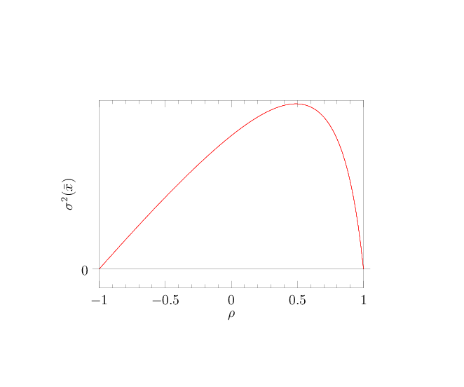
In the correlated case, and for fixed variances and , the variance smoothly depends on the correlation coefficient . It has maxima at and , only one of which is in the range . Notably, the relevant maximum is always at non-negative values of .
- (iii)
For , the variance vanishes identically, apart from the singular case and .
The generic form of as a function of is depicted in Fig. 4. In the presence of moderate correlations, therefore, anti-correlations are preferable over correlations in terms of reducing the variance of the average. Note that the result (39) is different from that of Eq. (8) in Ref. [20], since the definition of correlation coefficient used there is different from that in our situation of taking an average. Instead of measuring the correlation between and , their definition refers to the correlation of and .

The weights and of Eq. (38) are not restricted to be between zero and one. It is easy to see that for or , the average is in fact outside of the bracket . This seemingly paradoxical effect is easily understood from the optimal weights derived here. From Eq. (38) one reads off that the weights and leave the range as soon as resp. , depending on whether or , that is, only for strong positive correlations to the right of the maximum in Fig. 4. Thus, if the smaller of and has the smaller variance (and both are strongly correlated), the average is below both values. If the larger value has the smaller variance, the optimal average is above both values. The asymmetry comes here from the difference in variance. To understand this intuitively, assume for instance that and with strong positive correlations . It is most likely, then, that and deviate in the same direction from the true mean . Since , the deviation of should be generically smaller than that of . For , however, this is only possible if . This is illustrated in Fig. 5.
References
- [1] K. Binder and D. P. Landau, A Guide to Monte Carlo Simulations in Statistical Physics (Cambridge University Press, Cambridge, 2005), 2nd ed.
- [2] B. A. Berg, Markov Chain Monte Carlo Simulations and Their Statistical Analysis (World Scientific, Singapore, 2004).
- [3] W. Janke, in Computational Physics, edited by K. H. Hoffmann and M. Schreiber (Springer, Berlin, 1996), pp. 10–43.
- [4] C. Holm and K. Kremer, eds., Advanced Computer Simulation Approaches for Soft Matter Sciences, vol. 1 and 2 (Springer, Berlin, 2005).
- [5] M. Vojta, Rep. Prog. Phys. 66, 2069 (2003), URL http://dx.doi.org/10.1088/0034-4885/66/12/R01.
- [6] J. Zinn-Justin, Quantum Field Theory and Critical Phenomena (Oxford University Press, Oxford, 2002), 4th ed.
- [7] H. Kleinert and V. Schulte-Frohlinde, Critical Properties of -Theories (World Scientific, 2001), 1st ed.
- [8] D. Kandel and E. Domany, Phys. Rev. B 43, 8539 (1991), URL http://dx.doi.org/10.1103/PhysRevB.43.8539.
- [9] B. A. Berg and T. Neuhaus, Phys. Rev. Lett. 68, 9 (1992), URL http://dx.doi.org/10.1103/PhysRevLett.68.9.
- [10] F. Wang and D. P. Landau, Phys. Rev. Lett. 86, 2050 (2001), URL http://dx.doi.org/10.1103/PhysRevLett.86.2050.
- [11] M. E. Barber, in Phase Transitions and Critical Phenomena, edited by C. Domb and J. L. Lebowitz (Academic Press, New York, 1983), vol. 8, pp. 146–266.
- [12] A. M. Ferrenberg and R. H. Swendsen, Phys. Rev. Lett. 61, 2635 (1988), URL http://dx.doi.org/10.1103/PhysRevLett.61.2635.
- [13] B. Efron and R. J. Tibshirani, An Introduction to the Bootstrap (Chapman and Hall, Boca Raton, 1994).
- [14] H. Flyvbjerg and H. G. Petersen, J. Chem. Phys. 91, 461 (1989), URL http://dx.doi.org/10.1063/1.457480.
- [15] J. M. Hammersley and D. C. Handscomb, Monte Carlo Methods (John Wiley & Sons, 1964).
- [16] H. G. Ballesteros, L. A. Fernández, V. Martín-Mayor, and A. Muñoz Sudupe, Phys. Lett. B 387, 125 (1996a), URL http://dx.doi.org/10.1016/0370-2693(96)00984-7.
- [17] W. Janke and T. Sauer, J. Chem. Phys. 107, 5821 (1997), URL http://dx.doi.org/10.1063/1.474309.
- [18] M. Weigel and W. Janke, Phys. Rev. B 62, 6343 (2000).
- [19] M. Weigel and W. Janke, Phys. Rev. Lett. 102, 100601 (2009), URL http://dx.doi.org/10.1103/PhysRevLett.102.100601.
- [20] L. A. Fernández and V. Martín-Mayor, Phys. Rev. E 79, 051109 (2009), URL http://dx.doi.org/10.1103/PhysRevE.79.051109.
- [21] N. Metropolis, A. W. Rosenbluth, M. N. Rosenbluth, A. H. Teller, and E. Teller, J. Chem. Phys. 21, 1087 (1953), URL http://dx.doi.org/10.1063/1.1699114.
- [22] S. Brandt, Data Analysis: Statistical and Computational Methods for Scientists and Engineers (Springer, Berlin, 1998), 3rd ed.
- [23] A. D. Sokal, in Functional Integration: Basics and Applications, edited by C. DeWitt-Morette, P. Cartier, and A. Folacci (Plenum Press, New York, 1997), Proceedings of the 1996 NATO Advanced Study Institute in Cargèse, pp. 131–192.
- [24] M. B. Priestley, Spectral Analysis and Time Series (Academic Press, London, 1996).
- [25] A. D. Sokal and L. E. Thomas, J. Stat. Phys. 54, 797 (1989), URL http://dx.doi.org/10.1007/BF01019776.
- [26] K. Binder, in Phase Transitions and Critical Phenomena, edited by C. Domb and M. S. Green (Academic Press, New York, 1976), vol. 5b, pp. 1–105.
- [27] N. Madras and A. D. Sokal, J. Stat. Phys. 50, 109 (1988), URL http://dx.doi.org/10.1007/BF01022990.
- [28] K. G. Wilson, in Recent Developments in Gauge Theories, edited by G. ’t Hooft (Plenum Press, New York, 1980), Proceedings of the 1979 NATO Advanced Study Institute in Cargèse, pp. 363–402.
- [29] B. Efron, The Jackknife, the Bootstrap and Other Resampling Plans (Society for Industrial and Applied Mathematics [SIAM], Philadelphia, 1982).
- [30] A. M. Ferrenberg and R. H. Swendsen, Phys. Rev. Lett. 63, 1195 (1989), URL http://dx.doi.org/10.1103/PhysRevLett.63.1195.
- [31] W. Janke, in Proceedings of the Euro Winter School ” Quantum Simulations of Complex Many-Body Systems: From Theory to Algorithms”, edited by J. Grotendorst, D. Marx, and A. Muramatsu (John von Neumann Institute for Computing, Jülich, 2002), vol. 10 of NIC Series, pp. 423–445.
- [32] B. A. Berg, Comput. Phys. Commun. 69, 7 (1992), URL http://dx.doi.org/10.1016/0010-4655(92)90124-H.
- [33] U. Wolff, Phys. Rev. Lett. 62, 361 (1989), URL http://dx.doi.org/10.1103/PhysRevLett.62.361.
- [34] A. M. Ferrenberg and D. P. Landau, Phys. Rev. B 44, 5081 (1991), URL http://dx.doi.org/10.1103/PhysRevB.44.5081.
- [35] H. G. Ballesteros, L. A. Fernández, V. Martín-Mayor, and A. Muñoz Sudupe, Phys. Lett. B 378, 207 (1996b), URL http://dx.doi.org/10.1016/0370-2693(96)00358-9.
- [36] M. Hasenbusch, J. Phys. A 32, 4851 (1999), URL http://dx.doi.org/10.1088/0305-4470/32/26/304.
- [37] V. Privman, in Finite Size Scaling and Numerical Simulation of Statistical Systems, edited by V. Privman (World Scientific, Singapore, 1990), pp. 1–98.
- [38] W. Janke and R. Kenna, Phys. Rev. B 65, 064110 (2002), URL http://dx.doi.org/10.1103/PhysRevB.65.064110.
- [39] K. Binder, Z. Phys. B 43, 119 (1981), URL http://dx.doi.org/10.1007/BF01293604.
- [40] M. E. Fisher, Rev. Mod. Phys. 70, 653 (1998), URL http://dx.doi.org/10.1103/RevModPhys.70.653.
- [41] W. Janke and M. Weigel, Acta Phys. Polon. B 34, 4891 (2003).
- [42] M. Henkel, Conformal Invariance and Critical Phenomena (Springer, Berlin/Heidelberg/New York, 1999).
- [43] W. H. Press, S. A. Teukolsky, W. T. Vetterling, and B. P. Flannery, Numerical Recipes: The Art of Scientific Computing (Cambridge University Press, Cambridge, 2007), 3rd ed.
- [44] A. Pelissetto and E. Vicari, Phys. Rep. 368, 549 (2002), URL http://dx.doi.org/10.1016/S0370-1573(02)00219-3.
- [45] H. W. J. Blöte, L. N. Shchur, and A. L. Talapov, Int. J. Mod. Phys. C 10, 1137 (1999), URL http://dx.doi.org/10.1142/S0129183199000929.
- [46] K. Binder and D. W. Heermann, Monte Carlo Simulation in Statistical Physics — An Introduction (Springer, Berlin, 1988).
- [47] W. Janke, in Computer Simulations of Surfaces and Interfaces, edited by B. Dünweg, D. P. Landau, and A. I. Milchev (Kluwer Academic Publishers, Dordrecht, 2003), vol. 114 of NATO Science Series, II. Mathematics, Physics and Chemistry, pp. 111–135.
- [48] M. Weigel, Phys. Rev. E 76, 066706 (2007), URL http://dx.doi.org/10.1103/PhysRevE.76.066706.
- [49] M. Weigel and M. J. P. Gingras, Phys. Rev. B 77, 104437 (2008), URL http://dx.doi.org/10.1103/PhysRevB.77.104437.
- [50] P. Grassberger, Phys. Rev. E 56, 3682 (1997), URL http://dx.doi.org/10.1103/PhysRevE.56.3682.
- [51] M. Bachmann and W. Janke, Phys. Rev. Lett. 91, 208105 (2003), URL http://dx.doi.org/10.1103/PhysRevLett.91.208105.