New features of flat (4+1)-dimensional cosmological model with a perfect fluid in Gauss-Bonnet gravity
Abstract
We investigated a flat multidimensional cosmological model in Gauss-Bonnet gravity in presence of a matter in form of perfect fluid. We found analytically new stationary regimes (these results are valid for arbitrary number of spatial dimensions) and studied their stability by means of numerical recipes in -dimensional case. In the vicinity of the stationary regime we discovered numerically another non-singular regime which appears to be periodical. Finally, we demonstrated that the presence of matter in form of a perfect fluid lifts some constraints on the dynamics of the -dimensional model which have been found earlier.
pacs
04.20.Jb, 04.50.-h, 04.50.Kd, 98.80.-kI Introduction
Theories of gravity with the Gauss-Bonnet (GB) term as a correction to the Einstein term in the action have been actively investigated for more than 30 years [1, 2, 3, 4, 5]. This term appears as the first non-Einstein contribution in the extension of the General Relativity (GR) known as the Lovelock gravity [6] (the only theory that keeps the equations of motion to be the 2nd order differential equations), and string gravity [7]. In dimensions this term does not contribute to the equations of motion, and it can be important either in a combination with another fields (as it does in string theory) or in theories containing scalar function of the Gauss-Bonnet invariant (see, for example [8]; in this case we, however, have higher-order equations of motion).
For higher number of spatial dimensions the Gauss-Bonnet term is dynamically important. Moreover, in Lovelock gravity (in contrast with string gravity) this term is the only allowed non-Einstein contribution in () and () dimensions. This means that it is possible to study regimes where this term is not a small corrections to Einstein gravity, but equally important or even dominant.
In the end of 80th some important results in multidimensional cosmology with the Gauss-Bonnet term have been obtained including the analog of Kasner solution in a pure Gauss-Bonnet gravity [3]. Further studies reveal interesting differences between ()-dimensional case (this is the lowest number of dimensions for GB term to contribute) and higher-dimensional cosmology. This includes differences in the form of power-law solutions [3, 10], noncontinuity between vacuum solutions and solutions with matter (in () flat case with non-zero matter density the limit may not coincide with vacuum solutions [12]). Some of the differences can be extended to higher-order Lovelock corrections (at least in a flat case [13]). Other example of particularity of () case is severe fine-tuning needed for smooth evolution from high density (where GB term dominates) to low density (when Einstein gravity is restored) – such evolution requires three of four Hubble parameters to be equal with high precision [14]. This result have been obtained numerically in the theory which includes both GB and Einstein terms, so abovementioned results on dynamics with matter [12] (founded for a pure GB gravity) does not directly applicable to this case. Nevertheless, as we shell see, nonzero matter density can alter corresponding dynamics significantly.
The structure of the manuscript is as follows: first, we write down equations of motion for the model considered. Then, we analytically investigate stationary case and demonstrate exact solutions found. Then we switch to numerical studies and confirm by means of numerical recipes the reality of the previously found solutions as well as describe new oscillationary regime. Also we demonstrate (also via numerical methods) that the presence of matter in form of a prefect fluid lifts some constraints on the dynamics of the model considered. Finally, in the Conclusions we summarize the results found.
II Equations of motion
We consider a flat anisotropic metric in (4+1)-dimensional space-time. We are dealing with Einstein-Gauss-Bonnet gravity, and non-vacuum space-time. Lagrangian of this theory have a form
where is Ricci scalar, is the Lagrangian of matter fields and
| (1) |
is the Gauss-Bonnet Lagrangian.
We are working in the flat background, so the metric we considering has a form
| (2) |
We use perfect fluid with the equation of state as a matter source; after varying action obtained from (1) using the metric above and perfect fluid as a matter field, one can obtain the following equations of motion – there are dynamical equations and a constraint one. First dynamical equation has the form
where as usual , the rest of them could be obtained via cyclic index permutation. The constraint equation has a form
| (7) |
III Stationary solutions
The system of equations (II)–(7) has solutions of a particular type in which all Hubble functions are constant (and, correspondingly, scale factors expand or contract exponentially), so, we call them as stationary for brevity. Anisotropic exponential solutions in Einstein-Gauss-Bonnet gravity with matter were particularly studied in [9] under some assumptions. Here we study maximally anisotropic case:
For solution to be a stationary one it is necessary that right-hand sides of field equations
do not depend on time. This means that we need
| (8) |
i. e. one of a two conditions should be satisfied:
- 1.
— matter is a cosmological constant; or
- 2.
— volume element is constant.
As in this section we have some results for an arbitrary number of spatial dimensions, we write down the equation of motion for a flat -dimensional stationary case (i.e. neglecting all time derivatives):
| (9) |
| (10) |
For we have investigated only -dimensional space () with () and have obtained the following solutions:
- 1.
where satisfies condition
- 2.
where .
- 3.
where
and satisfies condition
- 4.
and satisfies condition
- 5.
where and satisfies condition
- 6.
For a general solution was investigated for arbitrary number of dimensions. If we express
and similarly for other products of Hubble parameters, we get the equations in the form
| (11) |
where
If and then we obtain that the general solution is any set of that satisfies the following conditions:
From this we can obtain a particular case of [9] where
It is interesting to note that from equations (11) in the case and we have only one condition to be satisfied
| (12) |
and that is in agreement with [10]. It can be also easily seen than the only case for a matter other than cosmological constant allowing a stationary solution in the pure Gauss-Bonnet gravity is of type. In this case the condition is
| (13) |
IV Numerical studies
Before describing regimes let us make some notes regarding our strategy. First of all, just like in previous papers where we numerically studied (4+1)- and (5+1)-dimensional Bianchi-I models [11, 12], we consider only models with positive initial (and in this section we again use dynamical in contrast with the previous section where due to parametrization used our Hubble function were constant). In (4+1) dimensions we specify 3 initial Hubble functions and calculate 4th using the constraint equation (7). This expression has a form
| (14) |
and here (and later) we use definition for (and later for ) to simplify notations: . Our goal is to study numerically the influence of non-zero matter density on the evolution scenario. We fix 3 Hubble parameters and change and the equation of state parameter . In this approach two different possibilities exist depending on the sign of denominator. If it is positive, we have no restriction on the initial value of matter density . If the denominator is negative, some maximal value of initial density exists (that maximal value satisfy ).
Solving system with respect to (, ) gives us values (, ) for stationary regime:
| (15) |
| (16) |
and that regime corresponds to the one, described analytically in the previous section.
IV.1 Singular vacuum regimes
We start with listing of possible regimes in (4+1)-dimensional vacuum Bianchi-I model. There are two possible outcomes for the past evolution – standard and non-standard singularities, and three for the future evolution – non-standard singularity, Kasner regime and recollapse. One can naively suppose that all six possible combinations of “past” and “future” regimes are occuring, but the reality is much more complicated. We summarized the trajectories in Table.
Table. Possible trajectories for vacuum (4+1)-dimensional GR+GB model
From
To
Design.
Avail.
Standard singularity
Kasner
I
+
Recollapse
II
+
Non-standard sing.
III
Non-standard. sing.
Kasner
IV
+
Recollapse
V
Non-standard sing.
VI
+
As it was noted in [14], type-I regime require fine-tuning of initial Hubble parameters, namely, three of them should be equal to each other. Recently [15] it was noted that sometimes the equality of two Hubble parameters is enough to achieve this type of regime.
In contradiction with [14], we failed to find type-III transitions. Authors of paper [14] claim they found them (around 1.5% of total number of trajectories), so keeping in mind possible numerical errors as well as different criteria to stop the integration process we can conclude that this regime is very rare if exists at all (see also [15] for possible reasons behind this).
IV.2 Regimes in presence of matter
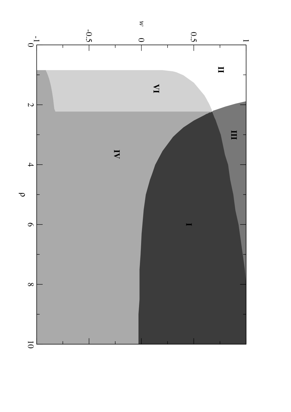

Since distinguishing of initial conditions with different signs of denominator in Eq. (14) is important for us, we treat these two cases separately. A typical transition diagram on the plane for the case of positive denominator is given in Fig. 1 (to be precise, it corresponds to the vacuum type-II case with positive denominator). White region corresponds to the type-II behavior, different grey regions correspond to VI, IV, III and I with increase of darkness of grey; they also denoted in figure.
From this figure we can see that type III evolution (which we have not seen in the vacuum case) and type I evolution (which occurs in the vacuum case only under very specific initial conditions) both appear as possible scenarios without any severe fine-tuning of initial conditions. As a result, all 6 possible scenarios listed in the Table 1, are possible when matter is taken into account.
In the transition diagram for the case of negative denominator we have the stationary regime at the right limit of the diagram if corresponding lies in the physical zone . In Fig. 2 as a way of example we present a typical example for negative (that is type-VI case with negative denominator). The situation at the limit line is as follows.
If and the “lifetime” of the type-II regime is increasing and asymptotically reaches infinity when . In Fig. 3 we presented the transition in question: Fig. 3(a) represents Hubble functions versus time for standard type-II regime (standard singularity to recollapse); one can see in Fig. 3(b), where we plot that the second singularity (that corresponds to recollapse) is isotropic one. With (and ) the situation changes according to Fig. 3(c); second singularity is still isotropic (Fig. 3(d)). Finally, when and , the stationary regime is reached (Fig. 3(e)).


If we have quite different behavior. Namely, it becomes periodical; in Fig. 4 we presented it. All through Fig. 4 we used the same value for density and decreased equation of state from in Fig. 4(a) down to in Fig. 4(e). One can see that with decrease of the equation of state the period and amplitude of oscillations are first increasing first, and then smoothly turn into quasi-stationary regime at . This means that small homogeneous perturbation of stationary regime does not necessary destroys nonsingular behavior, but turn it to periodic oscillations near the stationary point. If is less enough than then the described above periodical regime is not triggered and we have singular regime for any .

In case of the situation is different from described above. There are no periodic regimes in the vicinity of the stationary point. Any small perturbations of initial conditions needed for this solution ultimately leads to singular behavior. An example for regime transitions diagram for this case is plotted in Fig. 5. In general, we have not seen any periodic oscillations numerically with .
V Conclusions
We have considered dynamics of a flat -dimensional anisotropic Universe filled with an ordinary matter in Gauss-Bonnet gravity. Regarding singular regimes, we have founded that any of possible 6 different regimes (with 2 possible initial points in standard or nonstandard singularities, and 3 possible future outcomes – recollapse, nonstandard singularity or low-curvature Kasner solution) can be realized without severe fine-tuning of initial conditions. This means that some constraints of -dimensional dynamics in Gauss-Bonnet gravity found for vacuum regimes are lifter when matter is taken into account. Full description of all transition in both vacuum and matter cases is given in [15].
We have found also two nonsingular regimes – a stationary one with constant values of Hubble parameters and zero volume expansion rate (so, ) which have been found analytically for an arbitrary number of dimensions and oscillatory regime founded numerically in the vicinity of the stationary regime for -dimensional case. In our numerical studies we have seen this latter regime only for .
Acknowledgements
This work was partially supported by RFBR grant 08-02-00923.
References
- [1] F. Mller-Hoissen, Phys. Lett. 163B, 106 (1985).
- [2] J. Madore, Phys. Lett. 111A, 283 (1985); J. Madore, Class. Quant. Grav. 3, 361 (1986); F. Mller-Hoissen, Class. Quant. Grav. 3, 665 (1986).
- [3] N. Deruelle, Nucl. Phys. B327, 253 (1989).
- [4] T. Verwimp, Class. Quant. Grav. 6, 1655 (1989); G. A. Mena Marugán, Phys. Rev. D 42, 2607 (1990); ibid. 46, 4340 (1992).
- [5] N. Deruelle and L. Faria-Busto, Phys. Rev. D 41, 3696 (1990).
- [6] D. Lovelock, J. Math. Phys. 12, 498 (1971).
- [7] R. Metsaev and A. Tseytlin, Nucl.Phys. B293, 385 (1987).
- [8] K. Bamba, S. Odintsov, L. Sebastiani, and S. Zerbini, arXiv:0911.4390.
- [9] I. V. Kirnos and A. N. Makarenko, arXiv:0903.0083.
- [10] V. D. Ivashchuk, arXiv:0910.3426.
- [11] S.A. Pavluchenko and A.V. Toporensky, Mod. Phys. Lett. A24, 513 (2009) // arXiv:0811.0558
- [12] I.V. Kirnos, A.N. Makarenko, S.A. Pavluchenko, and A.V. Toporensky, arXiv:0906.0140
- [13] S.A. Pavluchenko, Phys. Rev. D80, 107501 (2009) // arXiv:0906.0141
- [14] R. Chingangbam, M. Sami, P. V. Tretyakov, and A.V. Toporensky, Phys. Lett. B661, 162 (2008) // arXiv:0711.2122
- [15] S.A. Pavluchenko, arXiv:1003.4892.