Bubbles of Nothing in Flux Compactifications
Abstract
We construct a simple flux compactification stabilized by a complex scalar field winding the single extra dimension and demonstrate an instability to nucleation of a bubble of nothing. This occurs when the Kaluza – Klein dimension degenerates to a point, defining the bubble surface. Because the extra dimension is stabilized by a flux, the bubble surface must be charged, in this case under the axionic part of the complex scalar. This smooth geometry can be seen as a de Sitter topological defect with asymptotic behavior identical to the pure compactification. We discuss how a similar construction can be implemented in more general Freund – Rubin compactifications.
I Introduction
Some time ago, Witten showed that the Kaluza – Klein vacuum suffers from a non-pertubative instability due to the semi-classical nucleation of so-called bubbles of nothing. Once formed, these smooth “boundaries” of space expand and soon engulf the whole of spacetime [1]. Such instabilities may be cause for concern regarding the viability of certain higher dimensional spacetimes as acceptable vacua. It is therefore necessary to consider the existence of analogous decay processes for perturbatively stable compactifications.
Flux compactifications [2] provide an elegant solution to the moduli problem in higher dimensional field theories [3, 4, 5, 6] as well as string theory [7, 8]. By stabilizing the extra dimensions with sufficiently high moduli masses, we can construct a model realistic enough to accommodate the low energy physics as well as a cosmological framework compatible with observations. These masses are induced by a flux potential, which depends on a discrete set of flux winding numbers. The diverse set of fluxes and associated winding numbers gives rise to the multitude of (meta)stable vacua known as the string landscape [9]. Although supersymmetric flux compactifications are known to be stable [10], the more phenomenologically interesting compactifications may enjoy/suffer from several instabilities, including decompactification [11, 12, 13] or more general transdimensional tunneling [13, 14], flux-transitions [15, 16, 17, 12, 18] and, as we will demonstrate here, nucleation of bubbles of nothing.11 1 Bubbles of nothing in flux compactifications have been recently discussed in [18] by matching different spacetime geometries across a codimension one brane. This is different from our present construction describing a geometry which is smooth everywhere, obviating the need to postulate the existence of domain walls. The bubble of nothing geometry asymptotic to a given flux compactification is a gravitational instanton which represents both the decay mediator and subsequent classical evolution of the metastable spacetime. This is the case for Witten’s bubble of nothing in the minimal Kaluza – Klein (KK) model [1].
The outline of the paper is as follows. In section II we review the original bubble of nothing. In section III we discuss how these bubble solutions can be obtained as the spacetimes of de Sitter topological defects in a simple flux compactification, where the extra dimension is stabilized by the presence of a winding complex scalar field. In section IV we obtain numerical solutions describing these bubbles of nothing. We conclude in section V and speculate on similar constructions in more general flux compactifications.
II The Original Bubble of Nothing
The bubble of nothing geometry introduced by Witten [1] is easily obtained from the five-dimensional Schwarzschild black hole,
| (1) |
It will be convenient for us to express this metric in terms of a new radial coordinate, , as
| (2) |
We can now Wick rotate two of the coordinates via
| (3) |
to yield
| (4) |
This is the bubble of nothing metric written in a somewhat unfamiliar gauge. (See the discussion in [19].) In the limit , it becomes
| (5) |
which is devoid of a conical singularity if we impose periodicity with . In this limit the slice degenerates onto a dimensional de Sitter space of size , representing the induced metric on the bubble surface.
In the limit of , the metric asymptotes to
| (6) |
which represents the cartesian product of Rindler space and a circle of circumference . The bubble of nothing geometry can therefore be regarded as a deformation of Rindler space (times a circle), whereby the horizon region near is replaced with a smooth tip consisting of , where is a cigar-shaped disk. This is illustrated in Fig. 1 below.


In order for this geometry to represent an instability of the Kaluza – Klein vacuum, it must have the same asymptotics as the pure compactification, in particular the same (zero) value of Schwarzschild mass. This can be seen to be the case in a number of ways. The KK compactification possesses the eleven isometeries of Poincaré, which are broken down to the seven in by the bubble of nothing (four translations are lost). This remaining symmetry is nevertheless larger than the five isometeries found in a generic Schwarzschild – Kaluza – Klein spacetime: , and so the mass of the bubble must be zero. Hence, barring any symmetry in place to prevent bubble nucleation, the KK vacuum is unstable.
III Bubble of Nothing in a Flux Compactification
In this section we will discuss the construction of a bubble of nothing geometry similar to that presented above, but with one crucial difference: we will stabilize the Kaluza – Klein radion. This is accomplished by introducing an axionic flux winding around the extra dimension. The simplest example of this type of flux compactification was described in [12] using the action for a complex scalar field given by
| (7) |
with and , where is the reduced Planck mass, and denotes the five-dimensional cosmological constant. We now review the results of [12].
III.1 The flux vacua
To begin, we shall constrain the magnitude of the scalar field to lie at , leading to the effective action
| (8) |
where is the phase of . The equations of motion for this model are
| (9) |
| (10) |
where
| (11) |
is the energy momentum tensor. We will look for a solution of the form
| (12) |
where denote the coordinates, and the compact extra dimension is parameterized by the coordinate . We are interested in the case
| (13) |
i.e., in solutions with the extra dimension stabilized at a constant circumference . We shall also require that the four-dimensional slices are described by a spacetime of maximal symmetry whose scalar curvature is given by , with negative for the anti-de Sitter (AdS) case.
The solutions to the equations of motion for the scalar field Eq. (9) which are compatible with maximal spacetime symmetry are given by
| (14) |
The change of axion phase around the compact dimension must be an integer multiple of , and hence the various flux vacua are parameterized by the integer .
With these assumptions we arrive at the Einstein equations
| (15) |
| (16) |
which fix the values of and in terms of and the parameters of the original Lagrangian according to
| (17) |
| (18) |
We thus conclude from Eq. (17) that flux vacua exist for compactifications provided the cosmological constant is negative (). Eq. (18) then indicates that these compactifications always yield a anti-de Sitter spacetime, enumerated by the integer . Furthermore, it can be easily shown by studying the effective action associated with these models [12], that the above solutions are perturbatively stable. We will now investigate the possibility that there exist non-pertubative instabilities of this geometry22 2 Flux-changing instantons [12] have previously been shown to exist. Their relation to the bubble of nothing presented here will be discussed below., similar to the pure Kaluza – Klein bubble of nothing presented in the previous section.
III.2 The bubble of nothing as a de Sitter brane
A particularly useful description of our compactification is given by the following metric which covers a Rindler-like portion of the spacetime shown in Fig. (2) below:
| (19) |


Comparing with the right hand illustration in Fig. (2), consider a metric of the form
| (20) |
with boundary conditions
| (21) |
for , and
| (22) |
in the limit .
It is clear from this description that such a solution, if it exists, would have the appropriate asymptotics as to match to the flux compactification solution Eq. (19) at the conformal boundary, where we must additionally impose that the axion approach the form Eq. (14). Looking at the boundary conditions imposed above, one can see that the metric in Eq. (20) has the same structure at as Witten’s solution discussed previously in Eq. (4); we have a compelling ansatz for a bubble of nothing in this flux compactification.
Because the compact dimension in this solution closes smoothly at , one must introduce some dynamical object that is able to resolve the flux singularity on the surface of the bubble. We can accomplish this simply by examining our original Lagrangian for the complex scalar field in Eq. (7). The problem arises only if one insists on keeping the modulus of the scalar field finite near the surface of the bubble. The divergence of gradient energy is cured by allowing the scalar modulus to relax along the radial direction in such a way that it vanishes at the tip of the cigar-like geometry. This is the same regularization found on a global string (i.e. codimension two) solitonic solution associated with a complex scalar field.
Singular bubbles of nothing in were constructed in [20], yielding a bubble surface charged with respect to the stabilizing flux. The bubble, located where an fiber degenerates, is singular due to the required de Sitter D3 branes smeared on the base. Our aim is to find non-singular solutions using a solitonic rather than smeared point-like sources.
As pointed out in [12], our Lagrangian admits such solitonic solutions describing 2-branes charged with respect to the axion . We therefore conjecture that one should identify the solution described above, the bubble of nothing within our flux compactification, as a de Sitter solitonic 2-brane in a AdS spacetime. We prove in the next section that one can indeed find such smooth bubble geometries in our model by numerically solving the equations of motion using the ansatz described above.
Solutions for de Sitter branes as topological defects have been previously discussed in [21], whose numerical solutions introduced many characteristics found in our bubble of nothing. Here we give a different interpretation for these spacetimes in the context of flux compactifications. We illustrate such a bubble of nothing in Fig. (3) below.


IV The Bubble Solution
We begin by considering the action
| (23) |
with metric
| (24) |
and scalar field
| (25) |
The symmetry of the bubble of nothing is easily seen within this ansatz. We arrive at the equations
| (26) |
and
| (27) |
having denoted
| (28) |
The Einstein tensor then becomes
| (29) |
and the energy momentum tensor is given by
The equations of motion are then any three of the four equations
Because our ansatz is explicitly time-independent, the Lorentzian and Euclidean solutions are trivially related.
IV.1 Asymptotic Solution of the full equations
Before numerically solving the near-bubble region, we determine the asymptotic values of all functions, which can be done exactly. The solution below exhibits the expected backreaction on the scalar modulus, the KK radion, and the vacuum energy density.
| (30) |
| (31) |
where,
| (32) |
| (33) |
| (34) |
and we have introduced the parameter ,
| (35) |
Note that in the limit , so we recover the pure flux compactification geometry described in previous section (See Eqs. (17) - (18)).
IV.2 Near core expansion
We can Taylor expand the equations of motion about the tip of the cigar. This leaves two unknown boundary conditions, which we will use as shooting parameters. For they are and . The remaining terms are then completely specified:
| (36) | |||||
| (37) | |||||
| (38) |
We then numerically integrate the equations of motion outward from to obtain the functions pictured in Fig. (4). The numerical values for the parameters used are
| (39) |
which give the solution
| (40) |
where is the reduced Planck mass. The Euclidean action of this solution is given by
| (41) |
where the numerical solution was matched to the background in a box of circumference . Our chosen parameter values are rather generic, but we expect a large range of solutions to exist. In particular, we can smoothly deform our parameters and corresponding solution to match the bubble of Witten.
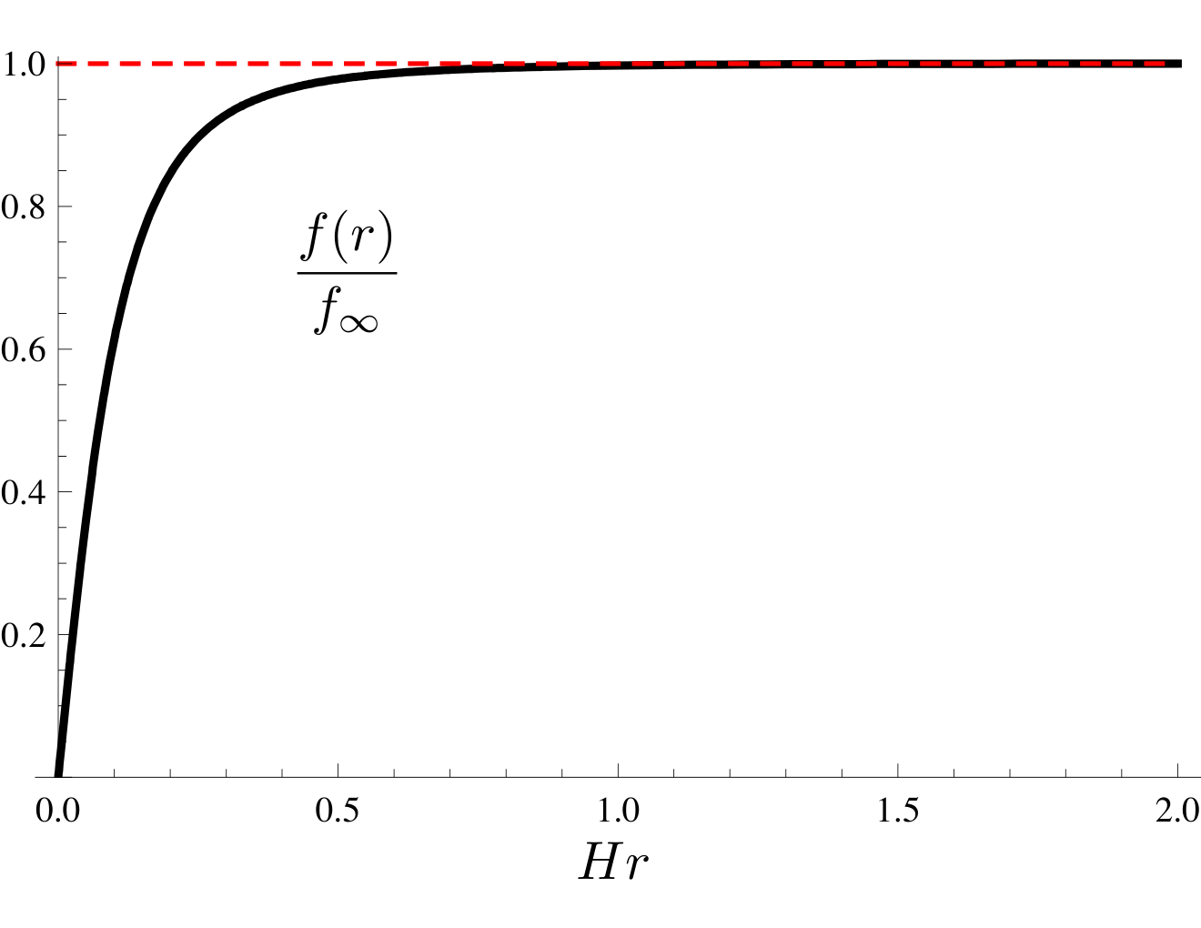
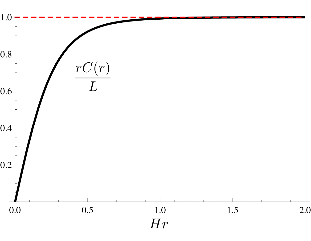
This is shown in the solution Fig. (5), where the chosen parameters are
| (42) |
which give the solution
| (43) |
The Euclidean action of this solution is given by
| (44) |
which is similar to the analogous action for Witten: . As seen in Fig. (5), the solution resembles that of Witten on scales smaller than , but then asymptotes to the AdS compactification far from the bubble.
V Conclusions
We have shown that a simple flux compactification exhibits an instability to the nucleation of bubbles of nothing. The key feature of this geometry is the flux through the compactification cycle at the conformal boundary, which demands a source wherever the cycle degenerates. Appropriately, the field theoretic model considered has solitonic 2-brane solutions which are charged with respect to the axionic flux stabilizing the extra dimension. One can construct a bubble of nothing in this context as the spacetime sourced by an “inflating” solitonic 2-brane whose worldvolume is given by a codimension-two de Sitter space (the surface of the bubble). We have obtained numerical examples of these bubbles which asymptotically match the pure compactification geometry.
We have presented our construction using the simplest field theory that possesses the minimal ingredients for the scenario to work, but we believe this kind of instability should be a generic feature of other non-supersymmetric flux compactifications. In particular, it will be straightforward to implement these ideas in a model based on a Einstein – Maxwell theory, where one finds a sizable landscape [5, 12] of , and vacua. As explained in [12], this theory possesses 2-brane solutions that could be used to construct instantons which interpolate between vacua of differing flux numbers. One can then extend this model to an Einstein – Yang – Mills – Higgs theory [3]. The new degrees of freedom incorporated in this model allow for smooth codimension-three solitonic 2-branes. One should then be able to find a magnetically charged de Sitter 2-brane with the correct asymptotics, similar to those in [22]. This type of bubble represents a significant departure from existing constructions, since the degenerating sphere is of dimension . One consequence of this topology is that spin structure will not play a role in excluding the instability. We are currently studying such solutions and will present our results in a separate publication.
An alternate perspective of the solutions presented here is as the critical case of a flux-changing instanton whose final vacuum has zero flux. Typical flux-changing transitions do not exhibit large backreaction on the spacetime geometry, provided one considers the nucleation of a single-charge brane, i.e., small relative changes in flux. On the other hand, the bubble of nothing corresponds to the extreme case, where the brane acts as a sink for all the flux found in the asymptotic compactification. It is not surprising that the effect on the geometry is drastic, since a zero-flux vacuum is unstable to collapse. One can see this in our model by examining the effective theory for the KK radion, which in the absence of flux is parameterized solely by the contribution from the negative bulk cosmological constant. The resulting tachyonic potential is divergent as one approaches zero-size compact dimension (See [12]). This suggests that one should be able to understand the bubble of nothing from a purely point of view by including the field as a new scalar degree of freedom in the effective theory. Such a solution may appear singular from the four-dimensional perspective, but this is just an artifact of the dimensional reduction, much like the case of Witten’s bubble [19].
The bubbles of nothing considered here affect many otherwise stable flux vacua. One should consider this instability as a new decay channel whose end result is a type of terminal vacuum, a vacuum without a classical spacetime. This is clearly relevant for any program undertaking the assigning of probabilities to different vacua in the landscape, the so-called measure problem. (See for example, [23] and references therein.)
VI Acknowledgments
We would like to thank Jaume Garriga, Oriol Pujolas and Alex Vilenkin for very helpful conversations and discussions. J.J.B.-P. would like to thank the Theory Division at CERN for its hospitality and support in the early stages of this work. J.J.B.-P. is supported in part by the National Science Foundation under grant 06533561. B.S. is supported in part by Foundational Questions Institute grant RFP2-08-26A.
References
- [1] E. Witten, “Instability Of The Kaluza – Klein Vacuum,” Nucl. Phys. B 195, 481 (1982).
- [2] M. R. Douglas and S. Kachru, “Flux compactification,” Rev. Mod. Phys. 79, 733 (2007).
- [3] E. Cremmer and J. Scherk, “Spontaneous Compactification Of Space In An Einstein Yang-Mills Higgs Model,” Nucl. Phys. B 108, 409 (1976).
- [4] P. G. O. Freund and M. A. Rubin, “Dynamics Of Dimensional Reduction,” Phys. Lett. B 97, 233 (1980).
- [5] S. Randjbar-Daemi, A. Salam and J. A. Strathdee, “Spontaneous Compactification In Six-Dimensional Einstein-Maxwell Theory,” Nucl. Phys. B 214, 491 (1983).
- [6] M. Gell-Mann and B. Zwiebach, “Space-Time Compactification Due To Scalars,” Phys. Lett. B 141, 333 (1984).
- [7] S. B. Giddings, S. Kachru and J. Polchinski, “Hierarchies from fluxes in string compactifications,” Phys. Rev. D 66, 106006 (2002).
- [8] S. Kachru, R. Kallosh, A. D. Linde and S. P. Trivedi, “De Sitter vacua in string theory,” Phys. Rev. D 68, 046005 (2003).
- [9] R. Bousso and J. Polchinski, “Quantization of four-form fluxes and dynamical neutralization of the cosmological constant,” JHEP 0006, 006 (2000); L. Susskind, “The anthropic landscape of string theory,” arXiv:hep-th/0302219.
- [10] S. Weinberg, “Does Gravitation Resolve The Ambiguity Among Supersymmetry Vacua?,” Phys. Rev. Lett. 48, 1776 (1982); M. Cvetic, S. Griffies and S. J. Rey, “Nonperturbative stability of supergravity and superstring vacua,” Nucl. Phys. B 389, 3 (1993).
- [11] S. B. Giddings and R. C. Myers, “Spontaneous decompactification,” Phys. Rev. D 70, 046005 (2004).
- [12] J. J. Blanco-Pillado, D. Schwartz-Perlov and A. Vilenkin, “Quantum Tunneling in Flux Compactifications,” JCAP 0912, 006 (2009).
- [13] S. M. Carroll, M. C. Johnson and L. Randall, “Dynamical compactification from de Sitter space,” JHEP 0911, 094 (2009).
- [14] J. J. Blanco-Pillado, D. Schwartz-Perlov and A. Vilenkin, “Transdimensional Tunneling in the Multiverse,” arXiv:0912.4082 [hep-th].
- [15] S. Kachru, J. Pearson and H. L. Verlinde, “Brane/Flux Annihilation and the String Dual of a Non-Supersymmetric Field Theory,” JHEP 0206, 021 (2002).
- [16] A. R. Frey, M. Lippert and B. Williams, “The fall of stringy de Sitter,” Phys. Rev. D 68, 046008 (2003).
- [17] B. Freivogel and M. Lippert, “Evidence for a bound on the lifetime of de Sitter space,” JHEP 0812, 096 (2008).
- [18] I. S. Yang, “Stretched extra dimensions and bubbles of nothing in a toy model landscape,” arXiv:0910.1397 [hep-th].
- [19] J. Garriga, “Smooth creation of an open universe in five dimensions,” arXiv:hep-th/9804106.
- [20] G. T. Horowitz, J. Orgera and J. Polchinski, “Nonperturbative Instability of ,” Phys. Rev. D 77, 024004 (2008).
- [21] I. Cho and A. Vilenkin, “Gravity of superheavy higher-dimensional global defects,” Phys. Rev. D 68, 025013 (2003).
- [22] I. Cho and A. Vilenkin, “Inflating magnetically charged braneworlds,” Phys. Rev. D 69, 045005 (2004).
- [23] A. Vilenkin, “A measure of the multiverse,” J. Phys. A 40, 6777 (2007).