Responses of the Brans-Dicke field due to gravitational collapses

The Lagrangian of the Brans-Dicke theory with a scalar field becomes [1]

where $R$ is the Ricci scalar, $\phi$ is the Brans-Dicke field, and $\Phi$ is a minimally coupled scalar field with potential $V(\Phi)$. Here, $\omega$ is the Brans-Dicke coupling constant which is a free parameter of the theory.

The Einstein equation becomes as follows:

where the Brans-Dicke part of the energy-momentum tensors are

and the matter part of the energy-momentum tensors are

The field equations are as follows:

where

We use the double-null coordinates

assuming spherical symmetry, where $u$ is the retarded time, $v$ is the advanced time, and $\theta$ and $\varphi$ are angular coordinates.

We follow the notation of [15][10][11][12]: the metric function $\alpha$, the radial function $r$, the Brans-Dicke field $\phi$, and a scalar field $S\equiv\sqrt{4\pi}\Phi$, and define

The Einstein tensors are then given as follows:

Also, we can obtain the energy-momentum tensors for the Brans-Dicke field part and the scalar field part:

To implement double-null formalism into the numerical scheme, it is convenient to represent all equations as first order differential equations. Note that

The Einstein equations for $\alpha_{,uv}$, $r_{,uv}$, and the field equation for $\phi$ are then coupled:

where

After solving these coupled equations, we can write all equations:

including the scalar field equation

Now, equations of $\alpha_{,uv}$, $r_{,uv}$, $\phi_{,uv}$, and $S_{,uv}$ parts can be represented by first order differential equations. We can then implement the same integration scheme used in previous papers [11][12] to solve the Brans-Dicke theory. We used the second order Runge-Kutta method [16]. Tests of the convergence are provided in Appendix B.

We need initial conditions for all functions ($\alpha,h,d,r,f,g,\phi,w,z,S,W,Z$) on the initial $u=u_{\mathrm{i}}$ and $v=v_{\mathrm{i}}$ surfaces, where we set $u_{\mathrm{i}}=v_{\mathrm{i}}=0$.

We have gauge freedom to choose the initial $r$ function. Although all constant $u$ and $v$ lines are null, there remains freedom to choose the distances between these null lines. Here, we choose $r(0,0)=r_{0}$, $f(u,0)=r_{u0}$, and $g(0,v)=r_{v0}$, where $r_{u0}<0$ and $r_{v0}>0$ such that the radial function for an in-going observer decreases and that for an out-going observer increases.

First, we assume that the gravitation constant $G=1/\phi$ is asymptotically $1$. Then, $\phi(u,0)=\phi(0,v)=1$ and $w(u,0)=z(0,v)=0$.

We use a shell-shaped scalar field, and hence its interior is not affected by the shell. Thus, we can simply choose $S(u,0)=A$ and $\alpha(u,0)=1$. Also, $W(u,0)=h(u,0)=0$ holds. Then, since the asymptotic mass function [17]

should vanish at $u=v=0$, it is convenient to choose $r_{u0}=-1/2$ and $r_{v0}=1/2$.

We need more information to determine $d,g,z$, and $Z$ on the $v=0$ surface. We obtain $d$ from Equation (39), $g$ from Equation (40), $z$ from Equation (41), and $Z$ from Equation (42), respectively.

We can choose an arbitrary function for $S(0,v)$ to induce a collapsing pulse. In this paper, we use

for $0\leq v\leq v_{\mathrm{f}}$ and otherwise $S(0,v)=0$, where $v_{\mathrm{f}}$ is the width of the pulse and $A$ is the amplitude. Then we obtain

for $0\leq v\leq v_{\mathrm{f}}$ and otherwise $Z(0,v)=0$. This implements one pulse of energy ($T_{vv}\sim Z^{2}$) along the out-going null direction by a differentiable function $Z(0,v)$.

Also, from Equation (38), we can use $d=rZ^{2}/2g\phi$ on the $u=0$ surface and we obtain $d(0,v)$. By integrating $d$ along $v$, we have $\alpha(0,v)$.

We need more information for $h,f,w,$ and $W$ on the $u=0$ surface. We obtain $h$ from Equation (39), $f$ from Equation (40), $w$ from Equation (41), and $W$ from Equation (42), respectively. This finishes the assignments of initial conditions.

We choose $r_{0}=10$, leaving the three free parameters $(\omega,A,v_{\mathrm{f}})$, where $\omega$ is the Brans-Dicke coupling parameter, $A$ is the amplitude of a pulse of the scalar field, and $v_{\mathrm{f}}$ is the width of the pulse. Here, we assume that there is no potential term in the matter field side.

We report the simulation results in Figure 1. We fixed $A=0.75$ and $v_{\mathrm{f}}=20$, and varied $\omega=10,1,0,-1,-1.4,-1.6,-2,-10$. Note that if $\omega=-1.5$, because of Equation (6), the equation becomes singular.

Figure 1 contains contour diagrams of the radial function $r$ for each parameters. We plotted singularities, trapping (apparent) horizons, and Cauchy horizons.

• •

  If the radial function becomes $0$, since the $r=0$ curve is space-like and all equations become singular, it is reasonable to interpret this region as a singularity.

• •

  To define a black hole using local geometry, we may use apparent horizons [18][19] or trapping horizons [20] for an out-going observer, i.e., $r_{,v}=0$. If there is inflation at some point in space-time, the inflating region can be defined by an in-going observer, i.e., $r_{,u}=0$, so that the in-going observer sees an increase of the area function. We plotted two horizons: $r_{,v}=0$ and $r_{,u}=0$.

• •

  If an apparent horizon contracts to a singularity, we can find a null cutoff line where we cannot calculate, because we do not have sufficient information to determine this region via the singularity; hence, we can identify the region as a Cauchy horizon [18][19].

In this subsection, we list some interesting observations for Figure 1. In the next section, we interpret the observations.

1. 1.

   Eventually a black hole is formed, i.e., a space-like singularity and an apparent horizon are observed.

2. 2.

   If $|\omega|$ is sufficiently large, the causal structures become similar to each other and the apparent horizons are always space-like. See $\omega=10$ and $-10$ cases.

3. 3.

   As $\omega$ decreases, if $\omega>-1.5$, the apparent horizon approaches the event horizon in the time-like direction. See $\omega=1,0,-1,-1.4$.

4. 4.

   If $\omega<-1.5$ and $\omega$ is sufficiently small, the apparent horizon oscillates and eventually approaches the event horizon in the space-like direction. See $\omega=-1.6,-2$.

5. 5.

   If $\omega\gtrsim-1.5$, the causal structure can contain an instantaneously inflating region, i.e., there can exist an $r_{,u}=0$ horizon. As $\omega$ approaches $-1.5$, the $r_{,u}=0$ horizon appears from upper $u$ to lower $u$. Compare $\omega=-1$ and $\omega=-1.6$.

6. 6.

   If $\omega\lesssim-1.5$, the apparent horizon can shrink to a singularity and form a Cauchy horizon. However, eventually a black hole will be formed. See $\omega=-1.6$.

Observations $1,2,3,$ and $4$ pertain to asymptotic behaviors after the collapse of matter. We call them late time behaviors. Observations $5$ and $6$ pertain to fully dynamical behaviors during the gravitational collapse. We call them dynamical behaviors (Figure 2). We discuss and interpret the late time behaviors and dynamical behaviors in the following section.

From the work of previous authors using Brans-Dicke theory, we know that a gravitational collapse should lead to the emergence of an Einstein black hole asymptotically [21]. As the black holes emerge to Einstein black holes, some interesting observations can be made. To understand these observations, in this section, we discuss the large $|\omega|$ case and the $\omega\sim-1.5$ case independently.

Now we turn to a discussion of fully dynamical behaviors during the matter collapse. We have observed interesting behaviors of $r_{,v}=0$ or $r_{,u}=0$ horizons. These behaviors should be consistent with energy-momentum tensors. Therefore, in this section, we look at details of the energy-momentum tensors and energy conditions that cause the dynamical behaviors. We discuss two different cases, $\omega\gtrsim-1.5$ and $\omega\lesssim-1.5$.

To understand the dynamical behaviors, we plot the energy-momentum tensor components (Figure 5). For any observer whose four velocity is $n^{\mu}$, the observer feels the energy density by

Therefore, if an observer moves along an in-going null direction, the observer feels the energy density by $T_{uu}$; if an observer moves along an out-going null direction, the observer feels the energy density by $T_{vv}$. Note that the null energy condition is violated if $T_{uu}$ or $T_{vv}$ has a negative region.

Around horizons ($r_{,u}=0$ or $r_{,v}=0$), we can simplify Equations (37) and (38) by

We know that asymptotically $r_{,u}<0$ and $r_{,v}>0$; i.e., initially, an in-going observer sees a decrease of area and an out-going observer sees an increase of area. Using these observations, we remark on two cases where the null energy condition should be violated.

• •

  We can define the outer part of an $r_{,u}=0$ horizon if the sign of $r_{,u}$ changes from $-$ to $+$ along an in-going null direction; the inner part of an $r_{,u}=0$ changes its sign from $+$ to $-$ along an in-going null direction. Then, around the outer $r_{,u}=0$ horizon, $r_{,uu}$ should be positive, and hence $T_{uu}<0$.

• •

  If $r_{,vv}<0$ around the (outer) $r_{,v}=0$ horizon, the horizon is space-like; if $r_{,vv}>0$ around the $r_{,v}=0$ horizon, the horizon is time-like. Therefore, to see a time-like $r_{,v}=0$ horizon, $T_{vv}<0$ is required.

Note that, $T_{uv}$ component is related to the vacuum energy or cosmological constant term. Therefore, if $T_{uv}>0$, then it may cause an increase of the area; if $T_{uv}<0$, then it may cause a decrease of the area. We can write Equation (40) around the $r_{,u}=0$ horizon as

If there is inflation, an out-going null observer sees an increase of area. This requires that $r_{,uv}>0$, and hence $T_{uv}$ should be sufficiently large:

If the inflation tends to end, the opposite situation should occur and $T_{uv}$ should be sufficiently small so that $r_{,uv}<0$. Therefore, we need to check the sign of $T_{uv}$ components if there is an $r_{,u}=0$ horizon.

We study responses of the Brans-Dicke field due to gravitational collapses of scalar field pulses using numerical simulations. In this paper, we used the double-null coordinates to implement the numerical simulations.

If the absolute value of the Brans-Dicke coupling constant $|\omega|$ is sufficiently large, the responses of the Brans-Dicke field are negligible and eventually an Einstein black hole will be formed. However, if $\omega$ is sufficiently small such that the Brans-Dicke field becomes sufficiently dynamic, we can see fully dynamical back-reactions of the Brans-Dicke field.

If we supply a scalar field pulse, it will asymptotically form a black hole via dynamical interactions of the Brans-Dicke field. Hence, we observed the responses of the Brans-Dicke field by two different regions (Figure 2). First, we observed the late time behaviors after the gravitational collapse, which includes formations of a singularity and an apparent horizon. Second, we observed the fully dynamical behaviors during the gravitational collapse and viewed the energy-momentum tensor components.

For the late time behaviors, if $\omega$ is greater (or smaller) than $-1.5$, the Brans-Dicke field decreases (or increases) during the gravitational collapse (Figure 3). Since the Brans-Dicke field should be relaxed to the asymptotic value with the elapse of time, the final apparent horizon becomes time-like (or space-like) (Figure 1).

For the dynamical behaviors, we observed the energy-momentum tensors around $\omega\sim-1.5$. If $\omega\gtrsim-1.5$, the $T_{uu}$ component can be negative at the outside of the black hole. This allows an instantaneous inflating region during the gravitational collapse (Figure 5). If $\omega\lesssim-1.5$, the oscillation of the $T_{vv}$ component allows the apparent horizon to shrink (Figure 7). In this case, we could find a combination of initial conditions that allows a violation of weak cosmic censorship (Figures 9 and 10).

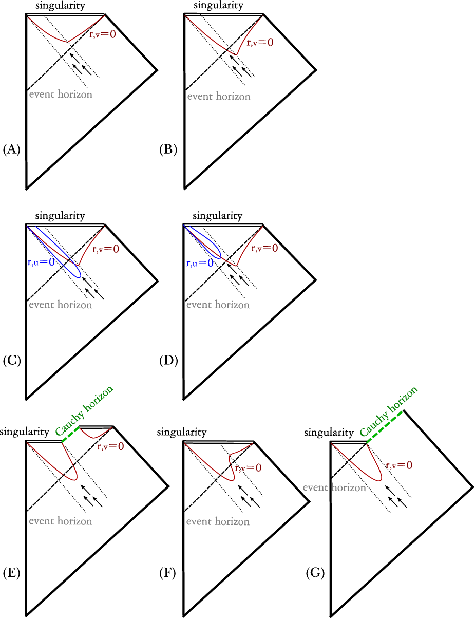
In Figure 11, we summarize and classify all solutions in this paper.

• (A)

  If $|\omega|$ is sufficiently large, the $r_{,v}=0$ horizon is space-like.

• (B)

  If $\omega>-1.5$ is sufficiently small, then the $r_{,v}=0$ horizon can be time-like after the matter collapse.

• (C), (D)

  If $\omega\gtrsim-1.5$, there can be $r_{,u}=0$ horizons. After the matter collapse, the $r_{,v}=0$ horizons are time-like.

• (E)

  If $\omega\lesssim-1.5$, we can find an initial condition that the $r_{,v}=0$ horizon shrinks to the singularity and eventually a space-like $r_{,v}=0$ horizon and a singularity appears. We can see a Cauchy horizon.

• (F)

  If $\omega\lesssim-1.5$, we also find an initial condition that the $r_{,v}=0$ horizon shrinks but not to a singularity. Then, we see an oscillation of the $r_{,v}=0$ horizon.

• (G)

  In $\omega\lesssim-1.5$ case, we can find an initial condition that the Cauchy horizon can be maintained infinitely.

Finally, we remark on some physical implications of our results.

First, in the $\omega\gtrsim-1.5$ limit, we could see a violation of the null energy condition for the $T_{uu}$ component. This condition is a necessary condition to induce a bubble universe using a false vacuum bubble [12]. It is necessary to check further calculations to ascertain whether this is in fact useful; but one lesson is that, in Brans-Dicke theory or similar type of theory, we may apply the back-reaction of a gravitational collapse to induce the negative $T_{uu}$ part.

Second, in the $\omega\lesssim-1.5$ limit, we could see a violation of weak cosmic censorship. Even though the Cauchy horizon extends infinitely, it is reasonable to speculate that a Schwarzschild black hole will be formed beyond the Cauchy horizon. However, it is also true that we cannot determine what happens beyond the Cauchy horizon. These situations were not observed using numerical simulations by previous authors [9]. Therefore, there should be further studies for this clear counterexample of weak cosmic censorship.

References

- [1] C. Brans and R. H. Dicke, Phys. Rev. 124, 925 (1961).
- [2] M. Gasperini, “Elements of string cosmology,” Cambridge, Cambridge University Press (2007).
- [3] L. Randall and R. Sundrum, Phys. Rev. Lett. 83, 3370 (1999) [arXiv:hep-ph/9905221].
- [4] J. Garriga and T. Tanaka, Phys. Rev. Lett. 84, 2778 (2000) [arXiv:hep-th/9911055].
- [5] Y. Fujii and K. Maeda, “The scalar-tensor theory of gravitation,” Cambridge, Cambridge University Press (2003).
- [6] B. Bertotti, L. Iess and P. Tortora, Nature 425, 374 (2003).
- [7] M. R. Setare, Phys. Lett. B 644, 99 (2007) [arXiv:hep-th/0610190].
- [8] A. G. Agnese and M. La Camera, Phys. Rev. D 51, 2011 (1995).
- [9]
M. A. Scheel, S. L. Shapiro and S. A. Teukolsky,
Phys. Rev. D 51, 4208 (1995) [arXiv:gr-qc/9411025];
M. A. Scheel, S. L. Shapiro and S. A. Teukolsky, Phys. Rev. D 51, 4236 (1995) [arXiv:gr-qc/9411026]. - [10]
T. Piran and A. Strominger, Phys. Rev. D 48, 4729 (1993) [arXiv:hep-th/9304148];
R. Parentani and T. Piran, Phys. Rev. Lett 73, 2805 (1994) [arXiv:hep-th/9405007];
S. Ayal and T. Piran, Phys. Rev. D 56, 4768 (1997) [arXiv:gr-qc/9704027];
S. Hod and T. Piran, Phys. Rev. Lett 81, 1554 (1998) [arXiv:gr-qc/9803004];
S. Hod and T. Piran, Gen. Rel. Grav. 30, 1555 (1998) [arXiv:gr-qc/9902008];
E. Sorkin and T. Piran, Phys. Rev. D 63, 084006 (2001) [arXiv:gr-qc/0009095];
E. Sorkin and T. Piran, Phys. Rev. D 63, 124024 (2001) [arXiv:gr-qc/0103090];
Y. Oren and T. Piran, Phys. Rev. D 68, 044013 (2003) [arXiv:gr-qc/0306078];
J. Hansen, A. Khokhlov and I. Novikov, Phys. Rev. D 71, 064013 (2005) [arXiv:gr-qc/0501015];
A. Doroshkevich, J. Hansen, I. Novikov and A. Shatskiy, arXiv:0812.0702 [gr-qc];
A. Doroshkevich, J. Hansen, D. Novikov, I. Novikov and A. Shatskiy, arXiv:0908.1300 [gr-qc]. - [11] S. E. Hong, D. Hwang, E. D. Stewart and D. Yeom, Class. Quant. Grav. 27, 045014 (2010) [arXiv:0808.1709 [gr-qc]].
- [12] J. Hansen, D. Hwang and D. Yeom, JHEP 0911, 016 (2009) [arXiv:0908.0283 [gr-qc]].
- [13] T. Chiba and J. Soda, Prog. Theor. Phys. 96, 567 (1996) [arXiv:gr-qc/9603056].
- [14] P. P. Avelino, A. J. S. Hamilton and C. A. R. Herdeiro, Phys. Rev. D 79, 124045 (2009) [arXiv:0904.2669 [gr-qc]].
- [15] R. S. Hamade and J. M. Stewart, Class. Quant. Grav. 13, 497 (1996) [arXiv:gr-qc/9506044].
- [16] W. H. Press, S. A. Teukolsky, W. T. Vetterling and B. P. Flannery, “Numerical Recipes: The Art of Scientific Computing,” 3rd ed. Cambridge, Cambridge University Press (2007).
- [17] B. Waugh and K. Lake, Phys. Rev. D 34, 2978 (1986).
- [18] S. W. Hawking and G. F. R. Ellis, “The large scale structure of space-time,” Cambridge, Cambridge University Press (1973).
- [19] R. M. Wald, “General relativity,” Chicago, Chicago University Press (1984).
- [20]
A. Ashtekar and B. Krishnan,
Living Rev. Rel. 7, 10 (2004) [arXiv:gr-qc/0407042];
S. A. Hayward, arXiv:gr-qc/9303006;
A. B. Nielsen and D. Yeom, Int. J. Mod. Phys. A 24, 5261 (2009) [arXiv:0804.4435 [gr-qc]]. - [21] S. W. Hawking, Commun. Math. Phys. 25, 167 (1972).
- [22] G. Kang, Phys. Rev. D 54, 7483 (1996) [arXiv:gr-qc/9606020].
- [23] R. d’Inverno, “Introducing Einstein’s relativity,” Oxford, Clarendon (1992).