JLAB-THY-10-1139
Electromagnetic form factors of the with D-waves
Abstract
The electromagnetic form factors of the baryon are evaluated within the framework of a covariant spectator quark model, where S and D-states are included in the wave function. We predict all the four multipole form factors: the electric charge , the magnetic dipole , the electric quadrupole and the magnetic octupole . We compare our predictions with other theoretical calculations. Our results are compatible with the available experimental data and recent lattice QCD data.
I Introduction
In the history of hadronic physics the nucleon was one of the first particles to have its internal structure experimentally uncovered. The nonpointlike character of the nucleon was suggested by the measurements of the proton anomalous magnetic moment. Around 1950, measurements disclosed an exponential falloff for the charge distribution, and three decades later the SLAC measurements showed that the corresponding charge form factor in momentum space coincided, almost perfectly, with the magnetic dipole form factor. This image of the proton proved to be a good approximation for low , the square of the four-momentum transfer, and was only superseded by the results from the Jlab polarization measurement in 1999 [2].
The study of the next baryonic state (the ) has been more challenging. Although the pure spin 3/2 and isospin 3/2 structure of the was clearly isolated from the background of the pion nucleon scattering experimental cross sections, its theoretical description is not yet totally clear. Quantum chromodynamics (QCD) emphasizes the three-quark state component, and historically the existence of the led to the introduction of color as a quantum number. Still, the issue on how much of the structure comes from a three-quark state, and how much is a molecularlike state of a nucleon and a pion, remains an open question.
Since the is a spin particle, its electromagnetic structure can be characterized by four form factors, namely the electric charge , magnetic dipole , the electric quadrupole and electric octupole form factors. The first two describe the charge and magnetic dipole distributions, while the last two measure the deviation of the first ones from the symmetric form [3]. At zero transferred momentum squared, , the form factors define the multipole moments: the charge , the magnetic moment , the electric quadrupole moment and the magnetic octupole moment . If the would simply be a completely symmetric state, with no quark D-states relatively to the quark pair (diquark), both and would vanish [4].
The unstable character of the (with a mean lifetime of 5.6) makes difficult to probe the electromagnetic properties of this particle/resonance. Until recently the available information on the structure came from the study of the reaction only. The dominance of the magnetic dipole moment in that reaction asserts the spin flip of a quark in the nucleon as the main process, but the magnitudes of the quadrupole contributions ( and ) indicate a small deformation of the [5].
The experimental information on the is restricted to the and magnetic moments [6, 7, 8, 9, 10, 11, 13, 12]. Even so, those results are affected by considerable error bars, due to the unstable nature of the and theoretical model uncertainties. This is particularly true for the magnetic moment [7]. See Refs. [8, 13] for a review. New experiments are in progress at MAMI [13] to extract more accurately with the help of reaction models based on hadronic degrees of freedom [12, 14, 15]. The scarce experimental information on is compensated by extensive theoretical studies within various frameworks [12, 15, 16, 17, 18, 19, 20, 21, 22, 23, 24, 25, 26, 27, 28, 29, 30, 31, 32, 33, 34, 35, 36, 37, 41, 42, 43, 44, 45, 38, 39, 40, 46, 47, 48, 49, 50, 51]. For a review see Ref. [4]. As for other observables, there is no other information, with the exception of the electric quadrupole moment , which was estimated using a connection to the transition quadrupoles [52]. For there is no experimental information related to the form factors. Even a very basic property like the electric charge radius is at present rather unknown, contrarily to what happens for the nucleon, where that quantity is accurately measured [53]. Our knowledge on the charge radius relies so far only on diverse theoretical model calculations [29, 32, 34, 44, 54, 55, 56, 57, 58, 59, 61, 62, 60, 46, 63]. There are also theoretical calculations of the quadrupole moment [29, 32, 61, 62, 31, 34, 63, 64, 65, 66, 67, 68, 50, 69, 70, 71, 72, 73].
Recently, the nature of the was explored in another direction, and under another light. Lattice QCD, the discrete version of the fundamental nonperturbative theory of the hadrons, was used to estimate the elastic form factors [74, 75, 76, 77], following the pioneer works of Bernard et al. [78] and Leinweber et al. [79]. The works [74, 77, 79] are based on the quenched approximation. The works [75, 76] are unquenched calculations, which include also sea quark effects. The results of the MIT-Nicosia group [74, 75, 76] were obtained for a wide range of , while the calculations of the Adelaide group [77] are performed for only one small value of (the limit case is impossible to reach for technical reasons) and extrapolated for to obtain the multipoles and the charge and magnetic radii. In particular for the background field method was used to calculate with a good accuracy the magnetic moment [78, 80, 81]. These methods were applied to pion mass values within the 0.31 GeV region and consequently some extrapolations are required [15, 82]. In the absence of direct experimental information lattice QCD provides the best reference for theoretical calculations for finite .
Motivated by the recent publication of lattice QCD data for the form factors [74, 75, 76, 77, 81], several models were also extended to determine those physical quantities. Calculations of the form factors were performed within the covariant spectator theory [4, 83] and also within a chiral Quark-Soliton model (QSM) [63]. Also, the magnetic octupole moment was estimated by Buchmann [3], using a deformed pion cloud model, and by Geng [50], using PT. Both and were estimated using QCD sum rules [70] and a covariant spectator quark model [83].
In this work we use a constituent quark model based on the covariant spectator formalism [84, 85, 5, 86] to predict the dependence of all four multipole form factors. Our results will be compared with the available experimental data, and the results from other models in the literature, as well as with recent lattice data. The electromagnetic form factors give us an insight into the internal structure. In particular the determination of the electric quadrupole and magnetic octupole moments gives information on how the is deformed, and on its size and shape. And this information is valuable, as we will conclude, to adequately constrain quark models. These in turn can be used to extrapolate and interpret lattice results.
The nucleon, as a spin 1/2 particle, has no electrical quadrupole moment, and the , a spin 3/2 state, emerges as the first candidate for a deformed baryon. A deformation (compression or expansion along the direction of the spin projection) would imply . The interpretation of as a signature of distortion matches well with our intuitive notion of deformation, based on the nonrelativistic limit of the Breit frame form factors. In that limit the Fourier transformation of the form factors gives the spatial distribution of charge or magnetic moment. We will therefore identify this notion as classical deformation. Recently, an alternative interpretation of distortion, based on transverse densities defined in the infinite moment frame, was introduced by other authors [76, 87, 88, 89]. Our calculations in this paper provide the basis needed for a forthcoming analysis of the deformation under the classical perspective and also in the newer perspective [90].
It is clear that the study of the form factors is a very interesting topic, even if experimentally arduous. The only experimental source of information about the deformation comes today from the quadrupole transition. However, this reaction depends on orbital angular momentum components in both the nucleon and of the [69, 91]. It is then very important to have an independent estimate of the angular momentum components in the (leading to a deformation) [92, 75, 76]. This is the main motive for our focus in this paper on the direct reaction.
In our previous work a first covariant spectator constituent quark model was developed for the nucleon, the transition and the [84, 85, 93, 5, 86, 94]. In the covariant spectator quark model a baryon is described as a system of three constituent quarks, with a off-shell quark free to interact with a electromagnetic field, while the quark-pair (diquark) acts as a spectator on-shell particle. Confinement is described effectively, with a quark-diquark vertex assumed to have a zero at the singularity of the three-quark propagator. The quarks are dressed, having an electromagnetic form factor with a behavior consistent with vector meson dominance. Within this first model we calculated the form factors considering the wave function parameterized simply by an S-wave state for the quark-diquark system. In this case only and have nonzero contributions because of the symmetry assumed for the system. In the work reported here we extend the previous model to the inclusion of the D-states, following Ref. [5]. It becomes then possible to predict, without further parameter fitting, nonzero results also for and . Although our results regard only the valence quark contributions, they compare well with a variety of lattice QCD data, besides the available experimental data.
We organize this paper in the following main sections: In Sec. II we introduce the basic definitions used to calculate the electromagnetic form factors. In Sec. III we review the covariant spectator quark model and present the wave function. In Sec. IV we derive the form factors within our model. In Sec. V we show the numerical results. Finally, in Sec. VI we draw some conclusions.
II electromagnetic form factors
The interaction of a photon with an on-mass-shell isobar, with initial four-momentum and final four- momentum , can be parameterized in terms of the electromagnetic current [95, 91]:
where is the mass, is the Rarita-Schwinger spin 3/2 state, , with the four possible charge values. The four functions () of define the four form factors [in appendix A, we discuss the general form of ()]. They can be combined to form the two electric and two magnetic multipoles, which have a direct physical interpretation: the electric charge (E0) and quadrupole (E2), and the magnetic dipole (M1) and octupole (M3) form factors, defined as [4, 91, 95]
| (2) | |||||
| (3) | |||||
| (4) | |||||
| (5) | |||||
where the dimensionless factor
| (6) |
was introduced. The static magnetic dipole (), electric quadrupole () and magnetic octupole () moments are defined in the limit, as
| (7) |
III Delta wave functions
In our model the wave function is described by an mixture of an S-state and two D-state components for the quark-diquark system
| (8) |
where and are respectively the admixture coefficients for the two D-states: D3 (quark core spin ) and D1 (quark core spin ). is the normalization constant. To characterize we took the covariant spectator theory for a quark and a on-mass-shell diquark system, as proposed in Ref. [5].
From its symmetry properties, the quark-diquark S-state (quark core and orbital angular momentum ) has the general form
| (9) |
as proposed in Refs. [85, 5]. In this equation is a scalar function describing the momentum distribution of the quark-diquark system in terms of the and the diquark moment, and respectively; is the polarization state associated with the diquark spin [93] (the polarization index was omitted in this short-hand notation) and is the Rarita-Schwinger state. The isospin- to isospin- transition operators are represented by () [85, 4, 15, 91], and is the spin-1 diquark state (a combination of and quarks). The isospin operator acts on the isospin states. (See Ref. [85] for details.) The normalization of the wave function (9) to unity implies for the scalar wave function the normalization condition
| (10) |
where and the covariant integral over the momentum is defined in Eq. (25) below.
The D-states in the spectator formalism were introduced and explained in detail in Ref. [5]. Their definition is made through the -state operator defined as
| (11) |
where
| (12) |
is the covariant generalization of the three-momentum in rest frame, and
| (13) |
generalizes the unity operator. The variables () describe the initial (final) momentum, and in the same way () refer to the initial (final) state.
Using the operator a generic spin 3/2 D-state is
| (14) |
It decomposes into a sum of two D-states, associated with the two possible spin states of the quark core, or (core-spin states ). To separate the two core-spin states we consider the two projection projectors:
| (15) | |||
| (16) |
where
| (17) |
The properties of the core-spin projectors are known in the literature [96, 97].
The amplitudes for the states associated to the core-spin (D1-state) and (D3-state) are defined as
| (18) | |||
| (19) |
where
| (20) | |||
| (21) |
As before, acts on the isospin states. For simplicity, in our notation the diquark polarization () and spin projections () are suppressed in the wave functions. Also , are scalar wave functions. The factor was introduced for convenience. The normalization of the wave functions is
| (22) |
and ensures that the wave function satisfies the charge condition,
| (23) |
The variable represents in the rest frame () and is the (quark) charge operator at . See Ref. [5] for more details about the D-states.
IV Current and Form Factors
Within the covariant spectator theory, the electromagnetic current in impulse approximation, can be written as in Refs. [84, 85, 5]
| (24) |
which sums in all intermediate diquark polarization and integrates over the diquark three-momentum
| (25) |
It also includes the symmetrization of the quark current. Following Ref. [84] the photon-quark interaction is represented by
| (26) | |||||
where is the nucleon mass and the isospin () and spin () operators acts on the initial and final states. The coefficients with are the quark form factors and function of . The explicit form of will be introduced later in Sec. V.
For numerical applications we define the isospin dependent functions and as
| (27) | |||
| (28) |
and is the isospin- matrix defined as
| (29) |
We can also write as , where is the diagonal matrix with the isospin projections: [32]. In the limit we use
| (30) |
The values of were fixed in Ref. [84] by the nucleon magnetic moments.
It is convenient also to define
| (31) |
Similarly as for and we suppress the tilde for .
As both the initial and final states depend of the diquark polarization with the same polarization index, the product of both polarization vectors factors out in the current (24). Then, since the initial and final state have the same mass () [84, 85, 93],
| (32) |
becomes
| (33) | |||||
Using Eq. (8) we can decompose the transition current into the contributions from the different components of the wave function:
| (34) | |||||
where the last three terms are corrections from the transitions between the same or different D-states. Those terms can be neglected if the admixture coefficients are small. We can write in a compact form
| (35) |
with explicit forms for the currents , and presented in Appendix B.
From the general form () and for the wave functions defined by Eqs. (9) and (18)-(19), we can write
| (36) | |||||
| (37) | |||||
| (38) | |||||
| (39) |
where is the overlap between the initial and final S-states,
| (40) |
and the other overlap integrals, between the initial S and each of the final D-states, are
| (41) | |||
| (42) |
with
| (43) |
The variable is defined by Eq. (12); the variable is defined the same way (just by replacing by ). The derivation of the previous expressions is presented in Appendix B.
In Eqs.(36)-(39), we chose to have in order to reproduce the charge of the . (the corrections due to the D-state to D-state transition are of the order of , and , as indicated by Eq. (34)).
The first observation to be made on the results (36)-(39) is that, to first order in and , the D-states do not contribute to . The second observation is that the D-states provide the only nonvanishing contributions to the electric quadrupole and magnetic octupole form factors, and (opening the possibility for a satisfactory selection of models for the D-states, otherwise specially difficult due to the overshadowing of their effects in by the dominant S-waves).
The definition of implies that when (see Ref. [5] for details). Since the wave functions are independent of in that limit, the angular integration of vanishes in the limit , and therefore the D-state overlap integrals vanish also. We stress that this result is model independent, since it is a consequence of the orthogonality between the S-state () and the D-states ().
Consider now the form factors and . They are proportional to , which is infinite for . But, as or are themselves proportional to , both form factors go to a finite value as and , ensuring no divergence. The proportionality simply comes from the specific dependence of the scalar wave functions on the quark momentum. The proof of that proportionality is done in Appendix C.
This is how a nonzero contribution from the D-state overlap integrals survives for each form factor, in spite of the orthogonality between S and D-states. This same behavior (overlap integral as ) was already observed also in the Coulomb quadrupole form factor of the reaction [5].
To conclude, the form factors and are a consequence of the D-states alone, and they depend on both the admixture coefficients, and , and the particular momentum dependence of the D-wave components of the wave function.
A remark about the predictions for the case can also be made: In our approach and , because the D-state to D-state transitions were neglected. Once those currents are included we may expect a nonzero, although rather small, contribution to .
The formulas obtained for the form factors are considerably simplified in the case . Since in that limit the integrals associated to transitions to the D-states vanish due to angular momentum, via , we are left with, setting
| (44) | |||||
| (45) | |||||
| (46) | |||||
| (47) |
(The factor from the normalization of was suppressed.) In these equations
The several moments, corresponding to each of the four multipole form factors, are calculated from Eqs. (7). Note that since the magnetic moment is defined by and and vanish at the origin, it follows that the magnetic moment is fixed by the S-state alone.
V Results
The algebraic results for the form factors given in the previous section were obtained within the covariant spectator formalism, independently of the specific model ingredients. In this section we start to specify the scalar wave functions and the quark current, required for an actual numerical application.
For the quark current we took the parameterization inspired on vector meson dominance (VMD) [84, 85, 5]:
| (48) |
where represents a light vector meson (or ), and is the mass of an heavy vector meson which simulates shorter range effects. The parameter was adjusted to give the correct quark density number in deep inelastic scattering [84, 85], . The coefficients and were fixed in a previous work to describe the nucleon elastic form factor data. We have , and [84]. The particular combination (48) with gives and therefore breaks isospin symmetry for , essential for a good description of the nucleon data. The anomalous magnetic moments and generate the nucleon magnetic moment exactly [84]. The parameterization (48) was applied to the nucleon [84, 94], electromagnetic form factors [4, 83] as well as to the three transition form factors [85, 5, 86, 94].
The scalar wave functions depend on the kinematic and dimensionless variable , as introduced in Refs. [84, 98, 4, 85, 5]:
| (49) |
| (50) | |||
| (51) | |||
| (52) |
The functions (50)-(52) were chosen for a good description of the data [85, 5, 86]. The coefficient in was determined by imposing the condition that the D1-state and the nucleon S-state are orthogonal [5].
In the applications we consider two different parameterizations for the wave function, both previously derived in the spectator formalism. By comparing the results of two models we can illustrate the sensitivity of the results to model building. The two parameterizations are equivalent with respect to the dominant S-state, but differ substantially in the D-state contributions. In both models the D-states give minor contributions for the quadrupole transition form factors, since they are basically dominated by the pion cloud contributions at low , which can be parameterized by a simple analytical structure [5]. The first model applied here, labeled Spectator 1 (Sp 1), was derived in Ref. [5] (and named model 4 there) to describe the transitions in the physical region. The D-states were calibrated by fitting the experimental data. The second parameterization, labeled Spectator 2 (Sp 2), was given in Ref. [86]. Although it has the same structure as Sp 1, it was adjusted to the lattice QCD data [99] for , in a pion mass region where the pion cloud effects are negligible, and afterwards extended to the physical pion mass point. The results for the physical region are therefore independent of the pion cloud mechanisms. This feature gives the latter model some robustness, making the procedure, in our opinion, more reliable, and indirectly, constrained by QCD as well. In the first model (Sp 1) there is an admixture of 0.88% for the D3-state and a larger admixture of 4.36% for the D1-state. In the Sp 2 model one obtains an admixture of 0.72% for both D3 and D1. These results supply us with the first quantitative idea of the sensitivity of the D-states to the fitting procedure. The D1-state, specially, shows to be strongly sensitive to that procedure.


| NRQM [29] | 0.74 | 1.06 | ||||||||
| MIT bag model [55] | 0.53 | 0.62 | ||||||||
| Skyrme [54] | 0.52 | 0.55 | 0.51 | -0.068 | 0.65 | |||||
| QSM [55] | 0.75 | 0.90 | ||||||||
| FT QM [56] | 0.56 | 0.70 | 0.67 | 0.03 | 0.71 | |||||
| RQM [57] | 0.520 | 0.523 | 0 | 0.523 | ||||||
| CQM (imp) [34] | 0.735 | 0.737 | 0 | 0.735 | ||||||
| CQM [34] | 0.766 | 0.766 | 0 | 0.766 | ||||||
| GP/Large- [59] | 0.7920.024 | 0.850.09 | 0.790.09 | -0.110.09 | 1.020.09 | |||||
| GBE [44] | 0.564 | 0.689 | 0 | |||||||
| QSM [63] | 0.768 | 0.794 | ||||||||
| QSM SU(3) [63] | 0.770 | 0.815 | ||||||||
| PT [50] | 0.3280.016 | |||||||||
| Spectator [4] | 0.33 | |||||||||
| Spectator 1 | 0.35 | 0.29 | -0.104 | 0.50 | ||||||
| Spectator 2 | 0.35 | 0.29 | -0.104 | 0.50 | ||||||
| Lattice: | ||||||||||
| Quenched [79] | 0.3970.088 | |||||||||
| Quenched [74, 100]a | 0.4770.008 | |||||||||
| Quenched Wilson [75, 76] | 0.4250.011 | |||||||||
| Dynamical Wilson [75, 76] | 0.3730.021 | |||||||||
| Hybrid [75, 76] | 0.4110.028 | |||||||||
| Quenched [77] | 0.4100.057 | 0.4100.057 | 0 | 0.4100.057 |
a Extrapolation to the physical point.


V.1 Electric charge form factor
The results for are shown in Fig. 1. The results for Sp 1 and Sp 2 are exactly the same because both models have the same S-state parameterization, and we chose . In the figure, for the case we compare our results with the physical extrapolation of the form factor from quenched lattice QCD data [74, 100]. For the other charge cases, in the absence of lattice data one can use exact isospin symmetry, which amounts to take
| (53) |
where for we used the dipole approximation of the lattice data [74, 100]. Although in quenched approximation this symmetry holds, there is no rigorous theoretical justification for it, since breaking of the isospin symmetry can be expected for , and was seen to be consistent with the nucleon data. In fact, the spectator models accommodate isospin asymmetry (through and ). This is why, in Fig. 2, where is compared directly with , the differences are more significant than what can be observed in Fig. 1 for . As expected, the disagreement between and increases with . Finally, in Fig. 3 we compare the results for with the neutron electric form factor. Note that the slope near is very similar, for both models and .
Comparing our calculations with the lattice data (extrapolated to the physical region) from Ref. [74, 100] we note, as observed previously in Ref. [4] where only S-states were taken, that both spectator models differ from the lattice data for low , but are significantly close to the lattice data at larger . Nevertheless, our models cannot be simulated by a pure dipole dependence as the lattice QCD data can, and one notices that they have a slightly slower falloff with , implying a smaller charge radius or, equivalently, a stronger charge concentration, than suggested by the lattice simulations. In our calculations the squared charge radius of the is 0.29 fm2 in both models, to be compared with 0.48 fm2 from the lattice simulation [74, 100].
V.1.1 Electric charge radius: comparison with other models
The analysis of the charge distribution is naturally done first in terms of the charge radius. For the charged states, the expansion of the charge form factor in powers of , ()
| (54) |
defines the charge squared radius as
| (55) |
For the case of neutral states (), , and we use
| (56) |
In some works Eq. (56) [with no normalization to included] instead of Eq. (55), defines the charge radius also for charged particles. The definition (55) has the advantage of being suitable to higher order form factors, namely , without loss of generality. For instance, for the proton, the electric charge and the magnetic dipole form factors have the same dipole dependence on at low , however with no normalization at as in Eq. (56), one is led to very different electric charge and magnetic dipole radii. In addition, with Eq. (55) the and the radii can be directly compared with . In particular, in a model with exact isospin symmetry [see Eq. (53] the charge radius is equal for all the charged states if Eq. (55) is used.
The results from our two models, together with a summary of the literature, is presented in Table 1. For a better interpretation of the results we write in the first column the prediction of each calculation for the squared charge radius of the proton, when it is available. Our prediction for the radius is 0.29 fm2. This number is below the value predicted by a variety of models.
The first estimate of the charge radius was based on NRQM and suggested fm2 [29], implying a larger spatial distribution for the than for the proton ( fm2). That effect was traditionally explained as a result of the repulsive hyperfine interaction of the quarks in spin-triplet state, in contrast with the attractive effect in the singlet state [29]. However, there was, at the time of this explanation, no direct experimental evidence of that fact.
The charge radius was also computed within the MIT bag model [55, 101]. One should mention for completeness other approaches, as a Skyrme model [54], a quark-soliton Model (QSM) [55], a field theory quark model (FT QM) [56], a relativistic quark model (RQM) [57], a constituent quark model (CQM) [69], a general parameterization of QCD combined with large- (GP/Large ) [59] a Goldstone boson exchange (GBE) model [44], a chiral soliton model (QSM) [63] and a chiral perturbation theory model (PT) [50]. Although the results differ from model to model, they all have in common the feature that the has a larger charge radius than the proton. The exception is the PT approach from Ref. [50].
The same trend is seen in CQMs. By taking a nonrelativistic CQM with two-body exchanges, Buchmann et al. [32] obtains for the electric radius squared,
| (57) |
where and are the proton and neutron squared radius. In the same model . Using recent values for the nucleon radii ( fm2; fm2) [53] one obtains fm2, which, in any case, is larger than .
The relation (57) was improved by Dillon and Morpurgo using a general parameterization (GP) of QCD [58] with corrections of the order of 10%-20%. Ameliorating upon Ref. [32], Ref. [34] establishes that the contributions of the impulse approximation are dominant to the charge radius, and that the two-body currents associated with the quark-antiquark pairs are only a small correction ( fm2). Using an operator method based on a GP [58] and the large- limit, Buchamnn and Lebed [59] related the four charge radii with the neutron and proton radii. Those results and their uncertainty are also shown in Table 1. In this case . A similar model, as the GBE model [44], predicts however a smaller charge radius ( fm2). Finally, a calculation within QSM suggests fm2 [63].
Interestingly, the most recent estimates of the electric squared radius [32, 34, 59, 44, 63] suggest fm2, slightly larger, but not significantly larger than the experimental result for the proton fm2. In general we can say that the several calculations in the literature predict .
Our prediction for the radius (0.29 fm2) is below all the model calculations identified above. In general these last ones also overpredict the lattice calculations values ( fm2 and fm2 from [74, 100]). Only the estimate of PT [50] is close to these lattice results.
As for the charge radius, it is interesting to note that it is very close to the neutron radius ( fm2) in our two models. This comes as no surprise, since, as noticed in Fig. 3, and the neutron electric form factor. have almost the same shape for low . The result is also consistent with partial quenched PT (PQPT) [46].
V.1.2 Electric charge radius: comparison with the lattice QCD results
Interestingly, our results are comparable in magnitude with the lattice QCD results in Refs. [75, 76, 77]. The lattice results shown in Table 1 correspond to the lowest pion mass taken by each method ( 300, 400 MeV).
It is expected that the lattice results for the charge radius increase as approaches the physical pion mass value, since it is what happens for the proton, where diverges as . In fact, the lattice data [77, 74, 75, 76] follows approximately the behavior of the proton charge radius as parameterized by PT in Ref. [102]. This is seen in the left panel of Fig. 4. The vertical line shown indicates the inelastic threshold for pion production, defined by . When this inelastic channel is crossed from above we can conjecture the suppression of charge radius below that point, as suggested by the magnetic moment studies within chiral effective field theory [82, 15, 75]. In the graph we include also the result of QSM in Ref. [63] at the physical point, fm2, which is close to the proton charge radius.
In the right panel of the Fig. 4 we illustrate that the lattice charge radius results [77], although comparable with the proton charge radius lattice data [103], are slightly larger, for the same lattice QCD conditions (lattice space fm) and approximation (quenched).
Some care must be taken in comparing model results like ours, and lattice QCD results. First, there are several methods to simulate the quark field in lattice, corresponding to different choices for the actions, as the Wilson (quenched or dynamical) [74, 75, 76, 105, 104], Clover [77, 103] or hybrid [75, 76] actions. The different choices lead to different results. Besides, lattice methods can differ in the calibration needed to make the connection with the physical limit. That can be done by adjusting the lattice spacing using the Sommer method [103], or the physical nucleon mass [105]. The two methods lead to very different predictions for the proton charge radius [103, 105].
To finish the discussion on the charge radius, we mention that the method from Ref. [46], based on quenched and partial quenched chiral perturbation theory, is useful to extrapolate lattice QCD calculations to the physical limit, and predicts results similar to the ones from our models Sp 1 and Sp 2.
V.1.3 Overview of the electric charge form factor
Apart from some deviation at low , our models give a reasonable description of the lattice data in all their range, when lattice uncertainties are considered.
Our two models (Sp 1 and Sp 2) gives the same result, because there are no D-state contributions for and we have used .
In comparison to other quark models, ours underestimate the charge radius, while it is very close to the lattice data from Refs. [74, 100, 75, 76]. We predict, as the lattice data does, a stronger charge concentration at the origin for the than for the proton. Still, we obtain a slightly weaker charge concentration than lattice QCD. The quality of the agreement with the quenched lattice data increases for high , where the meson cloud contribution should be smaller. This supports the idea that at least the valence sector is well described by our covariant spectator model. However, some corrections are expected from the pion cloud at low , and they are not yet included in our valence quark model. In principle, they will increase the charge radius. Another effect to be added in the future is the inclusion of the D-state to D-state transition. But this effect is expected to be small since it is proportional to the D-state to D-state contributions of the order of , and , with and already very small.
| Exp. [6, 7] | 7.342.49 | 3.54 | ||||||
| SU(6) | 7.31 | 3.65 | 0 | -3.65 | ||||
| QSM [63] | 6.36 | 3.09 | -0.18 | -3.45 | ||||
| Large [63] | 3.24 | |||||||
| PT [50] | 7.920.17 | 3.730.03 | -0.470.12 | -4.670.26 | ||||
| Large -PT [51] | 7.07 | 3.13 | -0.82 | -4.77 | ||||
| PQPT [46] | 7.58 | 3.79 | 0 | -3.79 | ||||
| SU(2) PT [48] | -0.97 | -5.51 | ||||||
| GBE [44] | 7.34 | 3.67 | 0 | -3.67 | ||||
| QCDSR [70] | 6.341.50 | 3.170.75 | 0 | -3.170.75 | ||||
| DM [43] | 7.16 | 4.80 | -3.29 | -4.93 | ||||
| Gauge/String Duality [45] | 5.81 | 3.04 | 0.27 | -2.51 | ||||
| model [41] | 7.66 | |||||||
| HCQM () [49] | 5.93 | 3.00 | 0.066 | -2.95 | ||||
| U-spin [47] | -1.760.08 | |||||||
| Spectator [4] | 6.71 | 3.29 | -0.12 | -3.54 | ||||
| Spectator 1 | 6.66 | 3.27 | -0.12 | -3.51 | ||||
| Spectator 2 | 6.66 | 3.27 | -0.12 | -3.51 | ||||
| Lattice: | ||||||||
| Background [80] | 6.860.24 | 1.270.10 | -0.0460.003 | -3.900.25 | ||||
| -extrapolation [82]a | 6.540.73 | 3.260.35 | 0.079 | -3.220.35 | ||||
| Quenched (ext) [74, 100]a | 3.040.21 | |||||||
| Quenched Wilson [75, 76] | 2.6350.094 | |||||||
| Dynamical Wilson [75, 76] | 2.350.16 | |||||||
| Hybrid [75, 76] | 3.050.24 | |||||||
| Quenched [77] | 5.280.92 | 2.640.46 | 0 | -2.640.46 | ||||
| Background [81]b | 4.850.16 | 3.150.08 | 0.00130.0210 | -2.420.08 |
a Extrapolation for the physical point; b Ref. [81] uses .
The lattice results from Refs. [75, 76, 77, 81] include no extrapolation to the physical point. The lattice results correspond respectively to MeV for quenched Wilson, MeV for the dynamical Wilson and MeV for the Hybrid action [75, 76]; MeV for quenched from Ref. [77] and MeV from Ref. [81].


| MIT bag model [55] | 0.38 | 0.46 | ||||||||
| Skyrme [54] | 0.47 | 0.39 | -0.16 | 0.71 | ||||||
| QSM [55] | 0.61 | 0.60 | ||||||||
| QSM [63] | 0.656 | 0.634 | ||||||||
| QSM SU(3) [63] | 0.665 | 0.658 | ||||||||
| CQM (imp) [34] | 0.656 | 0.656 | 0 | 0.656 | ||||||
| CQM [34] | 0.623 | 0.623 | 0 | 0.623 | ||||||
| GBE [44] | 0.752 | 0.689 | 0 | |||||||
| Spectator [4] | 0.37 | |||||||||
| Spectator 1 | 0.32 | 0.30 | 1.16 | 0.36 | ||||||
| Spectator 2 | 0.31 | 0.30 | 1.15 | 0.35 | ||||||
| Lattice: | ||||||||||
| Quenched [74, 100]a | 0.4120.049 | |||||||||
| Quenched Wilson [75, 76] | 0.2400.023 | |||||||||
| Dynamical Wilson [75, 76] | 0.2300.017 | |||||||||
| Hybrid [75, 76] | 0.2500.033 | |||||||||
| Quenched [77] | 0.4100.057 | 0.4100.057 | 0 | 0.4100.057 |
a Extrapolation for the physical point.
V.2 Magnetic dipole form factor
The magnetic dipole form factor results are shown in Fig. 5, for the four charged states. Only the magnetic moments of and are experimentally known, and their data points are represented in the graphs for , according to [9, 10, 11, 6, 8, 7]. The extrapolation of the quenched lattice QCD data to the physical point exists only for the case. In that case the dependence on of our results is directly compared to that extrapolation. For the other charge cases, in order to compare with the lattice QCD data we use the relation based on exact isospin symmetry
| (58) |
together with the dipole approximation for the lattice data. The result extracted from the lattice data [79] using PT [82] for is also shown in the graphs.
Our predictions for are very close to the lattice data. In detail, our results are 7% above the lattice data for low . However, the lattice errorbars are larger than the ones for the calculation, and our results are close to the limit of the errorbars. For high the agreement is very good. In the limit our results are consistent with both the experimental points and with the lattice data extrapolation from Refs. [82, 74, 100]. As found before in the calculation with S-waves only [4], the exception to this good agreement occurs in the case, where [82] predicts a sign different from ours. This disagreement is not problematic, since in that work the theoretical uncertainty was not explicitly evaluated, and is expected to be smaller relatively to the charged cases.
In Fig. 6 we compare the effect of the D-states to , for both models Sp 1 and Sp 2. We conclude that the effects of the D-states are small although they increase with . The small magnitude of these effects is easily understood from Eq. (37) with small admixture coefficients.
V.2.1 Magnetic moment: comparison with other models
Our predictions for the magnetic moments are and for both Sp 1 and Sp 2. The reason why both models lead to exactly the same result is that is determined only by the S-state parameterization, which is the same for the two models. There are some discrepancies between the different experiments, and the Particle Data Group [6] reports the interval of 3.7-7.5 for the magnetic moment. Our results are in good agreement with that result. Also the result for is consistent if the isospin symmetry is used to estimate the experimental value of .
The magnetic moment of is traditionally compared with the proton magnetic moment . In the heavy quark limit (static) approximation they coincide. The SU(6) prediction [17] implies that, when expressed in the nucleon magneton units (), the and the proton have the same magnetic moment []. Our results for the are in both models.
In a previous work [4], we compared our results for without D-waves with several formalisms, namely relativistic quark models [30], QCD sum rules [33, 35], chiral and soliton models [42, 31] and dynamical reaction models (DM) based on hadron degrees of freedom [15, 12]. Now we compare our calculations, with D-waves included, with a comprehensive update of the more recent results based on QSM [63], large- [63], SU(2) PT [48], PT [50], large -PT [51], PQPT [46], GBE [44], QCD sum rules [70], a quark models with sea quark contributions [41], a hypercentral quark model (HCQM) [49], a Gauge/String Duality model [45], a recent DM [43] and the U-spin symmetry [47]. For completeness. to this list we add the CQM with one and two-body currents [32]. The predictions for from all these works, together with our own results, are displayed in Table 2. The experimental and the SU(6) results are also included. Finally, we present the lattice QCD results [79, 82, 80, 74, 75, 76, 77].
In general, all the different models are consistent with the available experimental information.
The PDG interval for corresponds to and is . One has for assuming the isospin symmetry. The symmetric interval hold for , in the same approximation. Only Refs. [47, 48] for are clearly out of the interval.
As for the case, SU(6) and exact isospin symmetry predicts , and our models, and in general all models predict contributions an order of magnitude smaller than the magnetic moment of the charged or even zero (excluding the results from DM [43], SU(2) PT [48] PT [50] and large -PT [51]). When is not zero a negative value is frequently obtained, with a few exceptions. Note that the measurement of is technically extremely difficult, since on top of the very short lifetime, there is in addition the problem of tracking neutral particles. For all these reasons our knowledge of will probably be restricted in the near future to values from theoretical models and lattice simulations.
V.2.2 Magnetic moment: comparison with the lattice QCD results
Since the lattice simulations of the magnetic moment are performed for heavy quark masses, to compare with phenomenological models the extrapolation to the physical point is needed.
Fortunately, there are nowadays methods based on PT that can be used for such extrapolations [15, 82, 75]. The magnetic moment from Ref. [82] is the result of a chiral extrapolation. References [80, 74] use a simple functional dependence on the pion mass to extrapolate to the physical point. All the other lattice results in Table 2 refer to pions masses larger than the physical one.
The dependence of the magnetic moment on the pion mass is presented in Fig. 7 in addition to the result from models Sp 1 and Sp 2 at the physical point. The lattice data in that figure comprises the quenched results from [79, 80, 75, 76, 77], and the unquenched results from [75, 76] obtained with the Wilson and hybrid actions [81] using Clover fermions and also the background field method [78, 80, 81]. The chiral extrapolations of Cloet [82] using the pion loop corrections, and Lee [80] using a simple analytical form, is also on the graph. The inelastic point () is represented by the vertical line. The solid line in the figure corresponds only to the analytical part of the chiral extrapolation from Cloet et al. [82], but the analytical line and the full result lead to similar results for at the physical point [82] with an accuracy better that 10%. The extrapolation given by Cloet et al. compares well with our results.
The main conclusion from the figure is that there are large discrepancies between several lattice calculations. This makes harder to draw conclusions from the comparison of our results with the available lattice data. The unquenched results from Aubin et al. [81] for the exceed all the other calculations, including the analytical contribution to the chiral extrapolation [82]. Similarly to Ref. [80], in the Aubin results a significant deviation of the isospin symmetry (see Eq. (58)) is manifest in the and predictions. Note however that the Aubin results for , while different from the results, are similar to the results from other calculations. The significant violation of the condition , shows that the Aubin calculation violates strongly isospin symmetry, given by Eq. (58).
To understand the discrepancies between the different lattice calculations, it is important to realize that besides the extrapolation to the physical point, certain lattice calculation of demand an additional extrapolation of down to the point, given that the minimum lattice momentum is non-zero. The most common method uses a given analytical form for the extrapolation. A dipole [74], or an exponential falloff form [75, 76] have been used. Another possibility, used by the Adelaide group [79, 77, 103], applies the scaling between the electric charge form factor and the magnetic dipole form factor, . This assumption implies that the magnetic dipole radius squared is the same as the electric charge radius. Note, however that, although the scaling approximation is valid for the proton form factors [84], there is no reason to believe that it holds also for the system.
As a complete different alternative, the background field method [78, 80, 81] takes the three-quark system interacting at rest () with a static magnetic field. Considering the energy shift in the system, which is proportional to the magnetic dipole and also with the magnetic field, the magnetic moment is determined avoiding the uncertainty present in the extrapolation of the form factor method. The different results of [81] may be a consequence of the combination of a strong magnetic field with a not so large lattice volume used in the numeric lattice simulations.
The other problem to consider when comparing between and to different lattice calculations lies in estimating how the quenched approximation deviates from the results from the full QCD calculation, with the same pion mass.
In the SU(6) limit (exact SU(3) flavor symmetry) gives . This limit is obtained in quenched QCD when and light and strange quarks have the same mass, i.e. , with the kaon mass. In a recent quenched simulation [77] the SU(3) symmetry point corresponds to MeV ( GeV2) [77]. Below this point ( MeV) . This result can be understood analyzing the pion cloud contributions in quenched and in full QCD. As explained in Ref. [77], considering again , for MeV, those contributions are negative in quenched approximation while positive in full QCD.
Therefore, for in the region MeV, the quenched result underestimates not only full QCD, but even the the core contribution, which is already below the full QCD result. This is an artifact of the quenched approximation also observed in Refs. [80, 106].
As for , the extrapolations of Cloet [82] and Lee [80] give different signs. The Aubin result for MeV [81] is positive but the errorbars are so large that it can also be consistent with zero and negative values. Note that the results of Lee [80] are quenched and the results of Aubin [81] are unquenched.


V.2.3 Magnetic dipole radius
We define the magnetic dipole radius squared by means of the expansion of specified analogously to Eq. (55). The results of the magnetic dipole radius squared are listed on Table 3 for different models. At low they are similar to the ones obtained for the electric charge radius, suggesting a scaling between the electric charge and magnetic dipole form factors, as it was already observed for the proton form factors.
In the comparison between our results and others, the main difference is seen in the magnetic dipole radius, where we obtain a value larger than the radii predicted by all models discussed till this point. This can be just a consequence of the small value of for . As it happened for the electric radius, the results for the magnetic dipole radius of our two models, as well as the lattice QCD data, underestimate the results obtained with other quark models (see results of Refs. [63, 34, 44]). This can be a consequence of not including the pion cloud, expected to be important at low .
V.2.4 Overview of the magnetic dipole form factor
Our results indicate that the S-state contributions are dominant for the magnetic dipole form factors. In the previous section we saw that the same holds for the electric charge form factor. The D-states contribute only with small corrections. In spite of pion cloud effects not being included explicitly here, we predict magnetic dipole distributions similar to the lattice results. When compared with other quark models we predict a larger concentration of the magnetic dipole distribution at the origin.
| NRQM (Isgur) [64, 67] | -3.82 | -1.91 | 0 | 1.91 | ||||
| NRQM [67] | -3.63 | -1.79 | 0 | 1.79 | ||||
| Skyrme [68] | -3.39 | -1.21 | 0.94 | 3.12 | ||||
| Buchmann (imp) [32] | -2.49 | -1.25 | 0 | 1.25 | ||||
| Buchmann (exc) [32] | -9.28 | -4.64 | 0 | 4.64 | ||||
| PT [31] | -3.121.95 | -1.170.78 | 0.470.20 | 2.341.17 | ||||
| PT [50] | -1.051.29 | -0.940.58 | -0.860.94 | 0.780.78 | ||||
| QMCM [66] | -2.34 | -0.81 | 0.70 | 2.22 | ||||
| QSM [63] | -2.15 | |||||||
| QCDSR [70] | -0.04520.0113 | -0.02260.0057 | 0 | 0.02260.0057 | ||||
| GP(QCD) [52] | -7.024.05 | |||||||
| Spectator 1 | -4.08 | -2.04 | 0 | 2.04 | ||||
| Spectator 2 | -3.41 | -1.71 | 0 | 1.71 | ||||
| Lattice: | ||||||||
| Quenched [79] | -0.72.8 | -0.41.4 | 0 | 0.41.4 | ||||
| Quenched Wilson [76] | -0.810.29 | |||||||
| Dynamical Wilson [76] | -0.870.67 | |||||||
| Hybrid [76] | -2.06 |
| Spectator 1 | 0.58 | 0.53 | 0.21 | 0.74 | ||||
| Spectator 2 | 0.40 | 0.34 | 0.18 | 0.55 | ||||
| Lattice: | ||||||||
| Quenched Wilson [76] | 0.3360.096 | |||||||
| Dynamical Wilson [76] | 0.1340.106 | |||||||
| Hybrid [76] | 0.43 |


V.3 Direct comparison with lattice QCD
We have compared our results for the magnetic dipole form factor with the extrapolation to the physical pion mass point of the quenched lattice QCD data. But quenched data include pion cloud effects only partially, and lattice results based on quenched approximation are known to underestimate the full QCD result, as discussed. Fortunately, all form factors were recently also evaluated with unquenched methods. Those include sea quark effects from up and down quarks (Wilson action), and also from the strange quark (hybrid action) [75, 76]. For those calculations there are no extrapolations to the physical pion mass limit available. In these cases we could only compare our models directly to the published lattice data. Figure 8 shows the results for and corresponding to the lowest pion mass in each case: 411 MeV (quenched), 384 MeV (Wilson action) and 353 MeV (hybrid action). In addition to the results of Refs. [76] we include the point corresponding to MeV from Ref. [77].
Surprisingly, our two models also reproduce the magnitude of the lattice QCD data even in the nonphysical pion mass region. The agreement between our predictions for and the lattice data at low explains why the values obtained with our models are close to the lattice values, as seen in Table 3. Note that although different methods give very similar results for they exceed slightly the physical point (one data point from Ref. [77] is the exception, probably as a consequence of the small pion mass considered).
V.4 Electric quadrupole form factor
Because of Eqs. (36)-(37), the charge and magnetic dipole form factors are essentially determined by the S-state component of the wave function. But without D-states in the wave function the electric quadrupole form factor is identically zero. As such, measures a transition between the S-state and the D3-state (, ) of the [see Eq. (38)]. Differently said, the D3-state induces a deformation in the system that builds up a nonzero electric quadrupole proportional to the D3-state admixture parameter .
V.4.1 Electric quadrupole moment
The electrical quadrupole moment is defined as . The shape of the can be interpreted according to the sign of , if one relates in the Breit frame the charge distribution to the form factors in the nonrelativistic limit. For a positive charge, a deformation extended along the equatorial region () corresponds to an oblate distribution (pancakelike) and a deformation along the polar axis () to a prolate distribution (cigarlike). Alternative interpretations of deformation can be introduced, and give different insight on the structure [75, 76]. More details about this issue of deformation are presented in a separate work [90].


Our results for at are shown in Table 4. Since depends only on the state D3, is determined by which is (Sp 1) or (Sp 2). Besides, the D3-state admixture coefficents are not very different (0.88% versus 0.72%) and therefore both models give similar values for . In our case, because the D-state to D-state contributions were neglected. But nonzero although small contribution for may appear otherwise.
In Table 4 we make comparisons to other works, starting with nonrelativistic quark models (NRQM) e.g. the classic Isgur model [64]. In those models the quark D-states are a consequence of the hyperfine interaction in the presence of a confinement mechanism. Then was estimated in terms of the admixture coefficients for the symmetric, antisymmetric and with mixed symmetry components in the S and D-state wave functions, together with a confinement parameter associated to the spherical harmonic oscillator (interpreted as the quark core radius) [32, 29], and assuming, as we do here, that the transition between D-states is negligible.
In this type of NRQM description, where the valence quark degrees of freedom and the electromagnetic interaction are reduced to the impulse approximation (which includes only the one-body current), it was possible to relate the charge distribution with the neutron charge distribution [67, 107] according to
| (59) |
where is the neutron squared radius, and the index (imp) holds for impulse approximation (one-body current). Equation (59) is a parameter free relation, since it is independent of the admixture coefficients and of the confinement parameter. Considering a recent estimate fm2 [53], one has fm2, or , in close agreement to the result of Ref. [67]. Similar numerical results were obtained by Buchmann et al. [32] with a different combination of values for the admixture coefficients together with the confining parameter.
To estimate the nonvalence contribution for absent in the formulas above, Buchmann et al. [32] included two-body currents for the quark-antiquark production mechanisms, and obtained
| (60) |
In this case no D-state admixture is considered. Although it is a consequence of the constituent quark formalism, this result has again the feature of being parameter independent [32], and could even be obtained in the large limit [61]. Later, Eq. (60) was improved by means of a GP of QCD [52, 62, 58], for the inclusion of higher order terms. From the electric quadrupole data [52] the value was obtained. Note that this result, and already the result from Eq. (60) [32], are large when compared to the other calculations compiled in Table 4.
The other results in the literature are based on PT [31, 73, 50], on a quark-meson coupling model (QMCM) [66], on a Skyrme model [68], and more recently QSM [63] and QCD sum rules [70]. For completeness we mention as well calculations of PQPT in the heavy quark mass limit [46, 72], and relations between the electric quadrupole moments for different charge states [60, 71].
From lattice QCD there are earlier calculations from Leinweber [79], and recent simulations [75, 76, 63, 77] based on different approaches: quenched, dynamical Wilson ( and sea quarks) and hybrid action (also quarks included). The lattice results are also presented in Table 4.
Our model compares well with the NRQM from Refs. [32, 64, 67] based only on the valence quark degrees of freedom (see Table 4), although it overshoots the QCD sum rules [70]. Mixed descriptions, involving quarks and mesons, in particular pions, as degrees of freedom as PT [31, 50], QMCM [66] and QSM [63] suggest that the meson cloud can be important, although not as significant as Eq. (60) seems to imply.
V.4.2 Dependence of with
Before we compare our results with lattice QCD data we investigate the dependence of on . The results for are presented in Fig. 9, for the models Sp 1 and Sp 2, for all the charge cases. For the results are also compared with the more complete unquenched lattice QCD simulation (hybrid action) for the lightest pion mass available ( MeV) [76]. As a reference result we include also the PT calculation from [50] and the NRQM from Eq. (59). [The PT prediction for is out of the scale although the errorbars are consistent with our result (zero)]. The hybrid action considers and quarks as valence quarks, and , and as sea quarks. Therefore pion cloud contributions are included, although the results are not extrapolated to the physical pion mass.
In the left panel of Fig. 10 our models for electric quadrupole are compared with other lattice QCD methods, namely the quenched calculation with MeV and the dynamical Wilson action calculation with MeV, and again the hybrid action results for MeV. All the cases shown correspond to the smallest pion mass values of each method. In the same graph, also the lattice analytical extrapolations for assuming an exponential dependence in are included [Note the significant errorbars].
In the right panel of Fig. 10 we compare Sp 1 and Sp 2 with the dipole approximation of the model QSM from [63], that provides results for as function of . Additionally, the figure depicts the results from the analytical approximation of lattice QCD of Refs. [75, 76], as well as the NRQM and QCDSR [70] results for .
From Fig. 10 we conclude that our predictions are close to the hybrid action and the dynamical Wilson action results. Still, our results are larger, in absolute value, than the quenched data, particularly in the low region (note that the dynamical hybrid data are consistent with the Wilson and quenched data, within their statistical errors). The difference between our results and different lattice approaches seem to suggest that contrarily to the leading form factors and [4], the meson cloud effect may be important for . Also, the model QSM, where the contribution of the meson cloud (sea quark contributions) near is around 70% [63] falls faster that those models as increases. With the exception of Ref. [74] where an extrapolation to the physical point was published, there are no extrapolations of results for the physical point.
V.4.3 Overview of the electric quadrupole form factor
The electric quadrupole form factor is a measure of the deformation in the charge distribution, and is proportional to the transition coefficient between S and D3-states. Except for the lattice QCD calculations [74, 75, 76], and for the model QSM [63], previous studies of the dependence of the electric quadrupole form factors on are almost nonexistent. There are however predictions of several models at the photon point. Our model is consistent with most of these calculations based on valence quark degrees of freedom.
Our results agree also with the dynamical lattice QCD simulations with (Wilson and hybrid actions) for the lightest pion cases. Lattice QCD data seems to suggest that sea quark effects play a more important role for than for and , but the statistics must still be increased to allow more definitive conclusions.
The similarity of the D3-state parameterization in both our models Sp 1 and Sp 2 leads to very close results for the electric quadrupole form factor. We conclude that the quadrupole electric form factor is not suitable to discriminate between our models.


| QCDSR [70] | -0.0925 0.0234 | -0.0462 0.0117 | 0 | 0.0462 0.0117 | ||||
| GP [3] | -11.68 | -5.84 | 0 | 5.84 | ||||
| PT [50] | -4.079.49 | -2.034.76 | 0.059 0.036 | 2.264.52 | ||||
| Spectator 1 | -0.049 | -0.024 | 0.00084 | 0.026 | ||||
| Spectator 2 | -3.51 | -1.72 | 0.064 | 1.85 |
| Spectator 1 | 150 | 150 | 150 | 150 | ||||
| Spectator 2 | 1.2 | 1.1 | 2.0 | 1.2 |
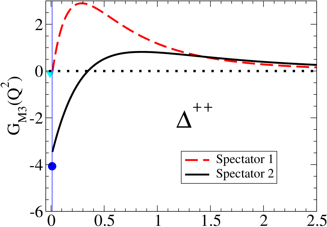
V.5 Magnetic octupole form factor
The third order form factor, , did not attract as much attention as the first order (, ) and the second order () form factors. Even for the magnetic octupole moment, , there is no experimental information whatsoever, although was estimated considering the earlier NRQM [29]. Interestingly, though, the lattice QCD simulations in Ref. [74] raised the question whether it is possible to determine the sign of accurately, or equivalently, with respect to the magnetic dipole distribution, whether the is prolate ( positive) or oblate ( negative). The first lattice QCD simulation [79] was not accurate enough to answer this question. The recent work of the MIT-Nicosia group [74] based on the quenched approximation increased the hope that or at least its sign can determined unequivocally by lattice QCD. This was a challenge for both MIT-Nicosia [76] and Adelaide groups [77]. The results from Ref. [77] (which are quenched) suggest a negative sign (i.e. a prolate distribution) for . Nevertheless, one has to check whether the results for are not significantly affected by the sign of the pion loop contributions, as it happens for (see discussion in Sec. V.2). One should note that those results correspond to large mass pions, and no physical extrapolation was performed yet.
From the theoretical point of view, the publication of lattice QCD results for triggered the application of quark models to compute and . Buchmann and Henley [3] using a CQM with pion cloud, two-body currents and the GP formalism [58] predicted fm3. The magnetic octupole was also recently predicted by QCD sum rules [70] and PT [50]. Predictions for , based on the SQM are expected for a near future [63]. PT predicts a nonzero octupole moment only at two meson loops level [31]. Within PQPT in the heavy quark mass limit at one meson loop level, one has [46, 72], consistently with the quenched QCD data from Ref. [77] for large pion mass values.
A summary of the predictions for , including our results from models Sp 1 and Sp 2, is presented in Table 6.
In the covariant spectator quark model, according to Eq. (47), depends only on the integrals , and the admixture coefficients and . For model Sp 1 one was , . As for model Sp 2, , . For the model Sp 1 the large contribution of the D1-state (4%) cancels the D3 contribution leading to an almost zero value to . This entails a dramatic difference between the results of models Sp 1 and Sp 2, as we can see from Table 6. Model Sp 1 gives negligible contributions for . The result from Sp 2 lies between the negligible predictions of QCD sum rules, and the large value of Buchmann [3] based on a pion cloud model and the GP formalism [58, 61, 3]. For completeness, and following the previous sections, the results for are also presented in Table 7.
The differences between models Sp 1 and Sp 2 for are clear from Fig. 11. For the cancellation between D1 and D3 contributions in model Sp 1 still exists, although it is not as spectacular as in the case. We note also the change of sign in Sp 2 for GeV2. It would be interesting in the future to compare the dependence of model Sp 2 with alternative models or with lattice data. The estimates of QCD sum rules [70], PT [50] and GP [3] for are also included in the graphs. For the we show the lattice data of Ref. [77] for the pion mass MeV at GeV2. In the graph we represent also the range of variation obtained in Ref. [74] from calculations with several pion masses.
The results for from model Sp 2 underestimate in absolute value the lattice QCD data point from Ref. [77] for MeV, but it is consistent with the central value of PT [50]. We note, although, that the errorbands are significant. The predictions of Sp 2 are also consistent the data from Ref. [74], within an interval associated with several pion masses. It will be interesting in the future to verify if the quenched approximation affects crucially and if the extrapolation to the physical point introduces significant corrections. To achieve that goal the errorbands must be reduced. At that point, Sp 2 can then be better tested.
We can conclude that, contrarily to the form factors analyzed before (electric charge, magnetic dipole and electric quadrupole) the magnetic octupole form factor is extremely sensitive to the D-state parameterization. As for our calculation enabling a decision in favor of Sp 1 or Sp 2, we consider model Sp 2 our best model, because it is better constrained, i.e. it is constrained by not only the experimental but also the lattice data of the reaction [86] (see discussion at the beginning of the section). Model Sp 2 predicts a much stronger deformation from the symmetric magnetic dipole distribution. It is also peculiar that the Sp 2 predictions for are similar to the predictions of . This implies an almost identical deformation for the electric charge and for the magnetic dipole distribution, if one uses the classical perspective of deformation.
A look at the magnetic octupole charge radius shows also a dramatic difference between the two models. Model Sp 2 predicts typical (although slightly large) values, but model Sp 1 breaks all the scales. That result might however be due to the equation used for , which is the analogue of Eq. (55), and breaks down in the limit when gets close to zero. But it might also be a consequence of the pion cloud effects not being explicit in this work.
V.5.1 Overview of the magnetic octupole form factor
Model Sp 2, which is our best model, gives a result for the magnetic octupole closer to the available lattice QCD data. We admit that model Sp 2 is not the last word in the wave function parameterization. Future lattice QCD simulations with increasingly smaller systematic errors may still discard the parameterization of Sp 2 [86]. Note that the quadrupole transition form factors can nowadays be experimentally measured for that reaction (the interaction time in is larger than in the reaction ). A direct test of the parameterization will be an even more accurate study of the reaction, once more precise data is provided. By using quadrupole form factors (electric and Coulomb) at the physical point [85, 5] or, in alternative, their data from lattice QCD [86, 75], the valence contributions of the wave function, and in particular the small D1 and D3-state contributions, can eventually be better constrained, to further refine our the predictions for the and form factors.
VI Conclusions
In this work we extended the spectator quark model to include the wave function D-states into the matrix elements of the electromagnetic current, in first order in the admixture coefficients of those states. This allowed us to evaluate all the four elastic form factors. We took two models previously calibrated by the two nucleon form factor data [84] and by the form factors for the reaction [5, 86]. The two models differ in the way they describe the quadrupole data. The first model (Sp 1) was derived by fitting the experimental data to the sum of the valence quark contribution with the pion cloud contribution [5]. The second model (Sp 2) was obtained by adjusting only the valence quark contributions to that reaction to the lattice QCD [86], data while still describing the physical data. Because in the last case we fixed the D-state parameters independently of the pion cloud mechanisms, in our view model Sp 2 is more reliable and robust than Sp 1.
Our predictions, based on the valence quark degrees of freedom alone, reproduce well the main features of the lattice results for and when extrapolated to the physical point, except for a some deviation at low . In particular, the agreement for high (say GeV2) is excellent, indicating that pion cloud effects (not included explicitly in our model) are small for high values. This confirms that the valence quarks are the dominant effect in the and form factors, as anticipated in a previous work [4] without the explicit contribution of the D-states. In the low region, however, our results for the suggest a smaller charge and magnetic charge radii, when compared with the proton. This can be a limitation caused by the absence of the chiral behavior (or pion cloud effects). Alternatively, it can also represent the real physical case if, as for the magnetic moment, there is a suppression of the charge radius due to the nonanalytical contribution of the inelastic region (). Further lattice QCD studies, preferably unquenched studies, are needed to clarify this point further.
The inclusion of the D-states in the wave function is required to explain the electrical quadrupole and magnetic octupole form factors. The D3-state (spin 3/2 state with an orbital D-wave) state is needed for a nonvanishing electric quadrupole moment for the . The D1-state (spin 1/2 with an orbital D-wave), as well as the D3-state (spin 3/2 with an orbital D-wave), generates nonvanishing contributions for the magnetic octupole form factor. By comparing our results with the available variety of lattice results, we conclude that valence quark contributions are of the same magnitude as the total result. This shows that to establish the magnitude of the contributions of the pion cloud to these observables requires more progress, with more accurate quenched and unquenched lattice data. In its absence for the near future [108], we may estimate the pion cloud effects similarly to what was done for the nucleon and the octet in Ref. [109]. That work concluded that, although significant for the nucleon magnetic moments, pion cloud effects give corrections of less than 8% for the quark anomalous magnetic moments.
Another interesting result to be further explored in the future is that contrary to , is very sensitive to model parameterization. This oversensitivity can be observed in the radius. The value of depends strongly on the D-states admixture and on the overlap between S and D1-states. We obtained an almost complete cancellation of in a particular model (Sp 1). If is in fact very small, then the study of D-state to D-state transitions may became important and should also be explicitly evaluated. Since the direct measurement of a third order multipole is technically difficult, a way out is, in our opinion, the use of the (experimental and lattice) data for an even more accurate determination of the D-state admixture following Refs. [5, 86], to predict as done here.
Our best model (Sp 2) gives for
| (61) |
These values correspond to the multipoles:
| (62) |
As the lattice QCD data for is still affected by a large uncertainty, our results for are independent predictions to be tested in the future.
The results (61)-(62), give an oblate deformation for the electric charge and magnetic dipole distributions, considering the classical interpretation of deformation. In Ref. [90] we compare this analysis with the one based on transverse density distributions.
The dependence of the form factor on that we obtain is very atypical, and it will be interesting if future lattice QCD calculations or alternative hadronic models may confirm our results. It can also happen that forthcoming lattice calculations may require a reparametrization of our model, which would affect in turn our results for the (where the quadrupole form factors, electric and Coulomb, are small and sensitive to the D-states.)
In the future, we can extend the model to the lattice QCD regime as suggested in Refs. [94, 86, 110]. That possibility was already explored in previous applications to the nucleon [94] and transition [94, 86]. The covariant spectator quark model defines a tool that can be used to extrapolate the lattice results both to the and to the physical pion mass limits. Another strength of this formalism is the possibility of its extension to the strange quark sector, enabling the application of the model to the octet and decuplet baryon systems. In particular, the application to the form factors [110] is very promising, since meson cloud effects (kaon cloud) are expected to be very small in that system. Our predictions could then be compared with lattice simulations nowadays performed at the strange quark physical mass [81, 77, 111].
Acknowledgments:
G. R. thanks Ross Young, David Richard and Anthony Thomas for helpful discussions. The authors thank also Peter Moron for helpful clarifications relative to Ref. [77] and Constantia Alexandrou for sharing the lattice data from Refs. [74, 100]. This work was partially supported by Jefferson Science Associates, LLC under U.S. DOE Contract No. DE-AC05-06OR23177. G. R. was supported by the Portuguese Fundação para a Ciência e Tecnologia (FCT) under Grant No. SFRH/BPD/26886/2006. This work has been supported in part by the European Union (HadronPhysics2 project “Study of strongly interacting matter”).
Appendix A Generic form to the current
Consider the electromagnetic current
| (63) |
The most general form, consistent with parity, G-parity [95], gauge invariance (current conservation) and the properties
| (64) |
reads
| (65) | |||||
The coefficients , , , , and are general functions of . Time reversal invariance implies that must be symmetric in the permutation (or ), and then we conclude that
| (66) |
Appendix B form factors
B.1 Current
B.2 Current
Consider Eqs. (9) and (19) in a compact notation
| (75) | |||
| (76) |
The transition between a S and a D3 state can be decomposed in two processes:
- •
S in the initial state (current )
- •
D3 in the initial state (current ).
In the following we will use the properties of the spin S-states (64) (S-state) and also
| (77) |
Note that the last identity holds for spin states based in a spin 3/2 core [85, 5]. Simple consequences of those relations are
| (78) |
Because the S and D3-states have the same core-spin, in general
although the result becomes zero for .
B.2.1 Transition S D3
The transition between an initial S-state (momentum ) and a final D3-state () can be written as
| (79) |
where the spin and polarization indices are suppressed for simplicity. We can write (79) as
| (80) |
where , and
| (81) | |||||
In the last equation we use the definitions of and from Eqs. (27)-(28).
Using the Gordon decomposition (69), we write the current (80) as
| (82) |
where is defined by Eq. (31), and
| (83) | |||
| (84) |
The expression for is given by Eq. (33).
To reduce the current to a form close to the standard one (), we work the spin algebra using the properties (64) and (77). We also use the covariant result of the integration in the azimuthal variable [5]:
| (85) |
where
| (86) | |||
| (87) |
The variable follows Eq. (13) and comes from Eq. (12) with replaced by . In the limit (initial and final state in the rest frame) is reduced to .
At the end, one has
| (88) | |||||
| (89) |
The common integral is defined by
| (90) |
B.2.2 Transition D3 S
The transition between an initial D3-state (momentum ) and a final S-state () can be written as
| (91) |
Once again, we suppress the spin and polarization indices for simplicity. We can write (91) as
| (92) |
where , . The operator is given by Eq. (81).
Using again the Gordon decomposition (69), we obtain
| (93) |
where is defined by Eq. (31), and
| (94) | |||
| (95) |
To reduce the current (93) to a form close to the standard one (), we work the spin algebra as before. We use again the covariant result of the integration in the azimuthal variable from Eq. (85) with the obvious replacement of (which implies , and ). One obtains
| (96) | |||||
| (97) |
where
| (98) |
One can prove now that:
| (99) |
One starts with the two integrals with explicit arguments written in the Breit frame. Then we conclude that the integrand of is a function of and the integrand of is a function of . Replacing we obtain identity in the Breit frame. As the integrals are covariant, the result holds for any frame.
B.2.3 Final result
Adding the two currents
| (100) |
we define two components ( and )
| (101) |
where
| (102) | |||||
| (103) |
with
| (104) | |||||
| (105) |
Considering the Fearing relation (68) and the Gordon decomposition (69) we can finally write
| (106) | |||||
From the previous relation and the definition of the form factors , we conclude that the form factors associated with , from Eq. (102), are
| (107) | |||
| (108) | |||
| (109) | |||
| (110) |
To evaluate the multipole form factors we consider the transformations (2)-(5). First we note that and . Then
It follows
| (111) | |||||
| (112) | |||||
| (113) | |||||
| (114) |
Take now the current from Eq. (103). Using the Gordon decomposition (69) and the form of from Eq. (105) one concludes that
| (115) | |||
| (116) | |||
| (117) | |||
| (118) |
From the previous equations it is easy to conclude that
And then,
| (119) | |||
| (120) | |||
| (121) | |||
| (122) |
The magnetic contributions vanishes for .
Finally we take the sum of the and components. Using the definition for , we are left with
| (123) | |||||
| (124) | |||||
| (125) | |||||
| (126) |
Note that the electric form factors include the electric factor , while the magnetic form factors include the factor . To achieve this final form it was essential to include the terms associated with : the result of the overlap between the spin functions associated with core spins 3/2 (S and D3). Note that, although vanishes for , as .
B.3 Current
The transition between a S and a D1 state can be decomposed into two processes:
- •
S in the initial state (current )
- •
D1 in the initial state (current ).
In the next calculations we use the properties of the spin S-states (64) (S-state) and D1-state :
| (129) | |||
| (130) |
See Ref. [5] for details.
B.3.1 Transition S D1
The transition between an initial S-state (momentum ) and a final D1-state () can be written as
| (131) |
We suppress the spin and polarization indicies for simplicity. We can write (131) as
| (132) |
where , and is given by Eq. (81).
B.3.2 Transition D1 S
We consider now the transition from D1 to S:
| (140) |
We conclude that
| (141) |
where the orthogonality was used again.
Working through the spin algebra,
| (142) |
we are left with
| (143) | |||
where
| (144) |
Similarly to Appendix B.2.2, we can prove that
| (145) |
B.3.3 Final result
Adding the two currents (138) and (143)
| (146) |
we obtain
| (147) | |||||
Using the Fearing-Nozawa relation (68) and the Gordon decomposition (69), we are left with
| (148) | |||||
Comparing the previous equation with Eq. (24), we conclude that
| (149) | |||||
| (150) | |||||
| (151) | |||||
| (152) |
Note that, although includes a factor , it is not singular. By definition of the integral vanishes as canceling the divergence in . The condition when is the result of the orthogonality between the states and .
Using the simple relations
| (153) | |||
| (154) |
we can write
Finally
| (155) | |||
| (156) | |||
| (157) | |||
| (158) |
In the limit only is different from zero.
B.4 All contributions
Each of the four form factors () is then the result of the three contributions calculated above:
| (159) |
The final result becomes
| (160) |
Appendix C Proof that
Consider the overlap integral
| (161) |
where represents an arbitrary (D3 or D1) D-state. The functions and are respectively the D-state and the S-state scalar wave functions written in terms of the dimensionless variable , as defined in Eq. (49). That is the only assumption made in this appendix. The function is defined by Eq. (43).
Although the integral is covariant the analysis can be considerably simplified in a particular frame. We consider then the rest frame of the final baryon (mass ):
| (162) |
where
| (163) |
In this frame we can write and . In the final baryon rest frame and has only spacial components.
It is now trivial to conclude () that
| (164) |
where we used , with . In the final baryon rest frame there is no dependence in , and only the scalar wave functions depend on .
The momentum dependence of the scalar wave appears through the functions , which become in the final baryon rest frame:
| (165) | |||
| (166) |
In the last equation we used . The previous equations show that the angular dependence appears only in the S-state wave function. To perform the angular integration (variable ) for we need only to consider the factor
| (167) |
where it is implicit that the integration is in the interval .
To proceed, we need to use the momentum dependence of . By taking the generic form
| (168) |
where is a integer (), is some normalization constant, and
| (169) |
where .
Factorizing according with
| (170) |
we can write
| (171) |
where
| (172) |
with For , for example: , , , etc.
The angular integration (167) is now considerably simplified
| (173) |
where the integral of the first term is zero , the second term vanishes because is the integral of an odd function (in a symmetric interval), and the same argument holds for the forth them (coefficient ). The next nonzero contribution appears only with the fifth term (coefficient ). As , the previous result can be written as
| (174) |
We still have to perform the integration in k. However, because as k, all integrals are well defined providing that the original integral is well defined. This means that integration in k preserves the decomposition presented above.
For small we need only to consider the leading dependence in of each term. Using , one has
| (175) |
Therefore
| (176) |
which finishes the proof.
Note that this derivation is independent of . The only constraint to be imposed is that the power in is sufficient to assure the convergence of the integral (in k). An alternative derivation is possible in a different frame, using also the properties of . For instance, in the initial baryon rest frame all angular dependence is in . Considering with the same form of from Eq. (168), we obtain the same limit for small using the procedure described before, as it should be.
References
- [2] C. F. Perdrisat, V. Punjabi and M. Vanderhaeghen, Prog. Part. Nucl. Phys. 59, 694 (2007) [arXiv:hep-ph/0612014].
- [3] A. J. Buchmann and E. M. Henley, Eur. Phys. J. A 35, 267 (2008) [arXiv:0808.1165 [hep-ph]].
- [4] G. Ramalho and M. T. Peña, J. Phys. G 36, 085004 (2009) arXiv:0807.2922 [hep-ph].
- [5] G. Ramalho, M. T. Peña and F. Gross, Phys. Rev. D 78, 114017 (2008) [arXiv:0810.4126 [hep-ph]].
- [6] W. M. Yao et al. [Particle Data Group], J. Phys. G 33 (2006) 1.
- [7] M. Kotulla et al., Phys. Rev. Lett. 89, 272001 (2002).
- [8] G. Lopez Castro and A. Mariano, Nucl. Phys. A 697, 440 (2002).
- [9] A. Bosshard et al., Phys. Rev. D 44 (1991) 1962; C. A. Meyer et al., Phys. Rev. D 38 (1988) 754.
- [10] B. M. K. Nefkens et al., Phys. Rev. D 18, 3911 (1978).
- [11] L. Heller, S. Kumano, J. C. Martinez and E. J. Moniz, Phys. Rev. C 35, 718 (1987); D. H. Lin, M. K. Liou and Z. M. Ding, Phys. Rev. C 44, 1819 (1991); P. Pascual and R. Tarrach, Nucl. Phys. B 134, 133 (1978);
- [12] W. T. Chiang, M. Vanderhaeghen, S. N. Yang and D. Drechsel, Phys. Rev. C 71, 015204 (2005) [arXiv:hep-ph/0409078]; D. Drechsel and M. Vanderhaeghen, Phys. Rev. C 64, 065202 (2001) [arXiv:hep-ph/0105060].
- [13] M. Kotulla, AIP Conf. Proc. 904 (2007) 203.
- [14] A. I. Machavariani, A. Faessler and A. J. Buchmann, Nucl. Phys. A 646 (1999) 231 [Erratum-ibid. A 686 (2001) 601].
- [15] V. Pascalutsa and M. Vanderhaeghen, Phys. Rev. Lett. 94, 102003 (2005) [arXiv:nucl-th/0412113].
- [16] K. Hikasa et al. [Particle Data Group], Phys. Rev. D 45, S1, (see pag. 482) (1992) [Erratum-ibid. D 46, 5210 (1992)].
- [17] M. A. B. Beg, B. W. Lee and A. Pais, Phys. Rev. Lett. 13, 514 (1964).
- [18] Y. A. Chao and R. K. P. Zia, Nuovo Cim. A 19, 651 (1974).
- [19] J. H. Kim, C. H. Lee and H. K. Lee, Nucl. Phys. A 501 (1989) 835.
- [20] G. Dillon and G. Morpurgo, Z. Phys. C 62, 31 (1994).
- [21] E. E. Jenkins and A. V. Manohar, Phys. Lett. B 335, 452 (1994) [arXiv:hep-ph/9405431].
- [22] S. T. Hong and G. E. Brown, Nucl. Phys. A 580, 408 (1994).
- [23] M. A. Luty, J. March-Russell and M. J. White, Phys. Rev. D 51, 2332 (1995) [arXiv:hep-ph/9405272].
- [24] M. K. Banerjee and J. Milana, Phys. Rev. D 54, 5804 (1996) [arXiv:hep-ph/9508340].
- [25] J. Linde and H. Snellman, Phys. Rev. D 53, 2337 (1996) [arXiv:hep-ph/9510381]; J. Linde, T. Ohlsson and H. Snellman, Phys. Rev. D 57, 5916 (1998) [arXiv:hep-ph/9709468].
- [26] P. Ha, Phys. Rev. D 58, 113003 (1998) [arXiv:hep-ph/9804383].
- [27] J. Franklin, Phys. Rev. D 66, 033010 (2002).
- [28] C. Hayne and N. Isgur, Phys. Rev. D 25, 1944 (1982).
- [29] M. M. Giannini, Rept. Prog. Phys. 54, 453 (1991).
- [30] F. Schlumpf, Phys. Rev. D 48, 4478 (1993) [arXiv:hep-ph/9305293].
- [31] M. N. Butler, M. J. Savage and R. P. Springer, Phys. Rev. D 49, 3459 (1994) [arXiv:hep-ph/9308317].
- [32] A. J. Buchmann, E. Hernandez and A. Faessler, Phys. Rev. C 55, 448 (1997) [arXiv:nucl-th/9610040]; A. J. Buchmann, in Baryons ’98, edited by D. W. Menze and B. Metsch (Word Scientific Singapore), p. 731 (1999) [arXiv:hep-ph/9909385].
- [33] F. X. Lee, Phys. Rev. D 57, 1801 (1998) [arXiv:hep-ph/9708323]; F. X. Lee, Phys. Lett. B 419, 14 (1998) [arXiv:hep-ph/9707411].
- [34] G. Wagner, A. J. Buchmann and A. Faessler, J. Phys. G 26, 267 (2000).
- [35] T. M. Aliev, A. Ozpineci and M. Savci, Nucl. Phys. A 678, 443 (2000) [arXiv:hep-ph/0002228].
- [36] B. O. Kerbikov, Phys. Atom. Nucl. 64, 1856 (2001) [arXiv:hep-ph/0003209].
- [37] S. Sahu, Rev. Mex. Fis. 48, 48 (2002).
- [38] H. Dahiya and M. Gupta, Phys. Rev. D 67, 114015 (2003) [arXiv:hep-ph/0211127].
- [39] B. Julia-Diaz and D. O. Riska, Nucl. Phys. A 739, 69 (2004) [arXiv:hep-ph/0401096].
- [40] G. S. Yang, H. C. Kim, M. Praszalowicz and K. Goeke, Phys. Rev. D 70, 114002 (2004) [arXiv:hep-ph/0410042].
- [41] C. S. An, Q. B. Li, D. O. Riska and B. S. Zou, Phys. Rev. C 74, 055205 (2006) [Erratum-ibid. C 75, 069901 (2007)] [arXiv:nucl-th/0610009].
- [42] H. C. Kim and M. Praszalowicz, Phys. Lett. B 585, 99 (2004) [arXiv:hep-ph/0308242]; H. C. Kim, M. Praszalowicz and K. Goeke, Phys. Rev. D 57, 2859 (1998) [arXiv:hep-ph/9706531].
- [43] A. I. Machavariani and A. Faessler, arXiv:0809.1303 [nucl-th]; A. I. Machavariani and A. Faessler, arXiv:0804.1322 [nucl-th].
- [44] J. He and Y. B. Dong, Commun. Theor. Phys. 43, 139 (2005) [arXiv:nucl-th/0404011].
- [45] K. Hashimoto, T. Sakai and S. Sugimoto, Prog. Theor. Phys. 120, 1093 (2008) [arXiv:0806.3122 [hep-th]].
- [46] D. Arndt and B. C. Tiburzi, Phys. Rev. D 69, 114503 (2004) [arXiv:hep-lat/0402029]; D. Arndt and B. C. Tiburzi, Phys. Rev. D 68, 114503 (2003) [Erratum-ibid. D 69, 059904 (2004)] [arXiv:hep-lat/0308001].
- [47] M. D. Slaughter, arXiv:0911.4756 [hep-ph].
- [48] F. J. Jiang and B. C. Tiburzi, Phys. Rev. D 81, 034017 (2010) [arXiv:0912.2077 [nucl-th]].
- [49] K. Thakkar, B. Patel, A. Majethiya and P. C. Vinodkumar, arXiv:1001.0849 [hep-ph].
- [50] L. S. Geng, J. Martin Camalich and M. J. Vicente Vacas, Phys. Rev. D 80, 034027 (2009) [arXiv:0907.0631 [hep-ph]].
- [51] R. Flores-Mendieta, Phys. Rev. D 80, 094014 (2009) [arXiv:0910.1103 [hep-ph]].
- [52] G. Blanpied et al., Phys. Rev. C 64, 025203 (2001).
- [53] C. Amsler et al. [Particle Data Group], Phys. Lett. B 667, 1 (2008).
- [54] B. Schwesinger and H. Weigel, Nucl. Phys. A 540, 461 (1992).
- [55] C. Gobbi, S. Boffi and D. O. Riska, Nucl. Phys. A 547, 633 (1992).
- [56] R. K. Sahoo, A. R. Panda and A. Nath, Phys. Rev. D 52, 4099 (1995).
- [57] N. Barik, P. Das and A. R. Panda, Pramana 44 (1995) 145.
- [58] G. Dillon and G. Morpurgo, Phys. Lett. B 448, 107 (1999).
- [59] A. J. Buchmann and R. F. Lebed, Phys. Rev. D 62, 096005 (2000) [arXiv:hep-ph/0003167].
- [60] A. J. Buchmann and R. F. Lebed, Phys. Rev. D 67, 016002 (2003) [arXiv:hep-ph/0207358].
- [61] A. J. Buchmann, J. A. Hester and R. F. Lebed, Phys. Rev. D 66, 056002 (2002) [arXiv:hep-ph/0205108].
- [62] A. J. Buchmann and E. M. Henley, Phys. Rev. D 65, 073017 (2002);
- [63] T. Ledwig, A. Silva and M. Vanderhaeghen, Phys. Rev. D 79, 094025 (2009) arXiv:0811.3086 [hep-ph].
- [64] N. Isgur, G. Karl and R. Koniuk, Phys. Rev. D 25, 2394 (1982).
- [65] D. Drechsel and M. M. Giannini, Phys. Lett. B 143 (1984) 329.
- [66] W. J. Leonard and W. J. Gerace, Phys. Rev. D 41, 924 (1990).
- [67] M. I. Krivoruchenko and M. M. Giannini, Phys. Rev. D 43, 3763 (1991).
- [68] J. Kroll and B. Schwesinger, Phys. Lett. B 334, 287 (1994) [arXiv:hep-ph/9405267].
- [69] A. J. Buchmann and E. M. Henley, Phys. Rev. C 63, 015202 (2000) [arXiv:hep-ph/0101027].
- [70] K. Azizi, K. Azizi, Eur. Phys. J. C 61, 311 (2009) arXiv:0811.2670 [hep-ph].
- [71] R. F. Lebed, Phys. Rev. D 51, 5039 (1995) [arXiv:hep-ph/9411204].
- [72] B. C. Tiburzi, Phys. Rev. D 71, 054504 (2005) [arXiv:hep-lat/0412025].
- [73] B. C. Tiburzi, Phys. Rev. D 79, 077501 (2009) arXiv:0903.0359 [hep-lat].
- [74] C. Alexandrou, T. Korzec, T. Leontiou, J. W. Negele and A. Tsapalis, PoS LATTICE2007, 149 (2007) [arXiv:0710.2744 [hep-lat]].
- [75] C. Alexandrou et al., Phys. Rev. D 79, 014507 (2009) [arXiv:0810.3976 [hep-lat]].
- [76] C. Alexandrou et al., Nucl. Phys. A 825, 115 (2009) [arXiv:0901.3457 [hep-ph]].
- [77] S. Boinepalli, D. B. Leinweber, P. J. Moran, A. G. Williams, J. M. Zanotti and J. B. Zhang, Phys. Rev. D 80, 054505 (2009) [arXiv:0902.4046 [hep-lat]].
- [78] C. W. Bernard, T. Draper, K. Olynyk and M. Rushton, Phys. Rev. Lett. 49, 1076 (1982).
- [79] D. B. Leinweber, T. Draper and R. M. Woloshyn, Phys. Rev. D 46, 3067 (1992) [arXiv:hep-lat/9208025].
- [80] F. X. Lee, R. Kelly, L. Zhou and W. Wilcox, Phys. Lett. B 627, 71 (2005) [arXiv:hep-lat/0509067].
- [81] C. Aubin, K. Orginos, V. Pascalutsa and M. Vanderhaeghen, Phys. Rev. D 79, 051502(R) (2009) arXiv:0811.2440 [hep-lat].
- [82] I. C. Cloet, D. B. Leinweber and A. W. Thomas, Phys. Lett. B 563, 157 (2003) [arXiv:hep-lat/0302008].
- [83] G. Ramalho, M. T. Peña and F. Gross, Phys. Lett. B 678, 355 (2009) [arXiv:0902.4212 [hep-ph]].
- [84] F. Gross, G. Ramalho and M. T. Peña, Phys. Rev. C 77, 015202 (2008) [arXiv:nucl-th/0606029].
- [85] G. Ramalho, M. T. Peña and F. Gross, Eur. Phys. J. A 36, 329 (2008) [arXiv:0803.3034 [hep-ph]].
- [86] G. Ramalho and M. T. Peña, Phys. Rev. D 80, 013008 (2009) arXiv:0901.4310 [hep-ph].
- [87] M. Burkardt, Int. J. Mod. Phys. A 18, 173 (2003) [arXiv:hep-ph/0207047].
- [88] C. E. Carlson and M. Vanderhaeghen, Phys. Rev. Lett. 100, 032004 (2008) [arXiv:0710.0835 [hep-ph]].
- [89] G. A. Miller and J. Arrington, Phys. Rev. C 78, 032201 (2008) [arXiv:0806.3977 [nucl-th]].
- [90] G. Ramalho, M. T. Peña and A. Stadler, in preparation.
- [91] V. Pascalutsa, M. Vanderhaeghen and S. N. Yang, Phys. Rept. 437, 125 (2007) [arXiv:hep-ph/0609004].
- [92] C. Alexandrou and G. Koutsou, Phys. Rev. D 78, 094506 (2008) [arXiv:0809.2056 [hep-lat]].
- [93] F. Gross, G. Ramalho and M. T. Peña, Phys. Rev. C 77, 035203 (2008).
- [94] G. Ramalho and M. T. Peña, J. Phys. G 36, 115011 (2009) [arXiv:0812.0187 [hep-ph]].
- [95] S. Nozawa and D. B. Leinweber, Phys. Rev. D 42, 3567 (1990).
- [96] M. Benmerrouche, R. M. Davidson and N. C. Mukhopadhyay, Phys. Rev. C 39 (1989) 2339.
- [97] H. Haberzettl, arXiv:nucl-th/9812043.
- [98] F. Gross and P. Agbakpe, Phys. Rev. C 73, 015203 (2006) [arXiv:nucl-th/0411090].
- [99] C. Alexandrou, G. Koutsou, H. Neff, J. W. Negele, W. Schroers and A. Tsapalis, Phys. Rev. D 77, 085012 (2008) [arXiv:0710.4621 [hep-lat]].
- [100] C. Alexandrou, private communication.
- [101] A. W. Thomas, Adv. Nucl. Phys. 13, 1 (1984).
- [102] E. J. Hackett-Jones, D. B. Leinweber and A. W. Thomas, Phys. Lett. B 494, 89 (2000) [arXiv:hep-lat/0008018].
- [103] S. Boinepalli, D. B. Leinweber, A. G. Williams, J. M. Zanotti and J. B. Zhang, Phys. Rev. D 74, 093005 (2006) [arXiv:hep-lat/0604022].
- [104] C. Alexandrou, G. Koutsou, J. W. Negele and A. Tsapalis, Phys. Rev. D 74, 034508 (2006) [arXiv:hep-lat/0605017].
- [105] M. Gockeler, T. R. Hemmert, R. Horsley, D. Pleiter, P. E. L. Rakow, A. Schafer and G. Schierholz [QCDSF Collaboration], Phys. Rev. D 71, 034508 (2005) [arXiv:hep-lat/0303019].
- [106] R. D. Young, D. B. Leinweber and A. W. Thomas, Nucl. Phys. Proc. Suppl. 128, 227 (2004) [arXiv:hep-lat/0311038]; D. B. Leinweber, A. W. Thomas, A. G. Williams, R. D. Young, J. M. Zanotti and J. B. Zhang, Nucl. Phys. A 737, 177 (2004) [arXiv:nucl-th/0308083].
- [107] J. M. Richard and P. Taxil, Z. Phys. C 26, 421 (1984).
- [108] K. Tsushima, and G. Ramalho, in preparation
- [109] F. Gross, G. Ramalho and K. Tsushima, Phys. Lett. B 690, 183 (2010) [arXiv:0910.2171 [hep-ph]].
- [110] G. Ramalho, K. Tsushima and F. Gross, Phys. Rev. D 80, 033004 (2009) [arXiv:0907.1060 [hep-ph]].
- [111] C. Alexandrou, T. Korzec, G. Koutsou and Y. Proestos, PoS LAT2009, 155 (2009) [arXiv:0910.3471 [hep-lat]].