Continuous-variable Quantum Key Distribution protocols with a discrete modulation

Quantum Key Distribution (QKD) appears to be the first real-world application of the fastly growing field of quantum information theory [1]. QKD protocols aim at distributing a secret key among distant parties, Alice and Bob, in such a way that an eavesdropper, Eve, cannot learn anything about the key except with an arbitrary small probability $\epsilon$. Since the proposal of the first QKD protocol in 1984 [2], most schemes have considered encoding information on two-level systems, such as the polarization of a single photon. In such schemes Bob would recover this information with photon counting techniques.

More recently, homodyne detection has been proposed to replace single photon counters. The main advantages of homodyne detection are its higher quantum efficiency and its greater technological maturity, both being consequences of the fact that homodyne detection is implemented with PIN photodetectors which are commonly used by the telecom industry. This is in sharp contrast with single photon detectors which are almost specific to QKD. In protocols relying on homodyne detection, which we refer to in the following as continuous-variable (CV) protocols by opposition to discrete-variable (DV) protocols, one must encode the information differently than in DV protocols: phase space replaces the traditional Bloch sphere describing the qubits used in BB84 for instance. The first CV QKD protocols were exploiting phase space as efficiently as possible by using coherent states with a Gaussian modulation [3] which is the modulation maximizing the mutual (classical) information between the input and the output of an Additive White Gaussian Noise (AWGN) channel. Such a channel models accurately the effect of typical optical fibers on the quadratures of the EM field. Using theorems about the optimality of Gaussian attacks, such schemes were proven secure against collective attacks [4, 5, 6] then later against general attacks [7] and were also successfully implemented [8, 9].

In order to reach significant transmission distances (with more than 3 dB losses), two different techniques have been proposed : reverse reconciliation where the key elements are a function of Bob’s measurement results [10, 11] and post-selection where Alice and Bob discard the data for which Eve has learnt too much information [12]. However, the analysis of post-selected schemes is quite involved their security has been established only against the restricted class of Gaussian attacks [13]. In this paper, we consider protocols with a reverse reconciliation but without post-selection.

In practice, CV QKD has many advantages on the implementation point of view, but up until now, it seemed restricted to smaller distances than photon-counting QKD, and for instance it was unable to distribute secret keys over more than 50 km. The reason for this comes from the difficulty to correct the errors between Alice and Bob’s data induced by the quantum channel. If this is not a problem in principle as one only needs to approach the Shannon capacity of a AWGN channel, it turned out to be quite difficult to realize in practice for a Gaussian modulation [14]. For this reason, using a discrete modulation instead of a continuous Gaussian modulation appeared as a possible solution as it greatly simplifies the error correction step. However, switching from a continuous to a discrete modulation opens new theoretical questions as the proof techniques used in [4, 5, 6] do not apply anymore. One therefore needs to develop a new approach to prove the security of CV QKD protocols with a discrete modulation. This was recently done in [15] for a protocol with a quaternary modulation. The new technique allows one to establish the security of the protocol when the quantum channel is linear. In particular, the noise added by the channel can be either Gaussian or non-Gaussian. Moreover, one advantage of the proof is that it only requires to estimate two experimental parameters, namaely the transmission $T$ and excess noise $\xi$ of the quantum channel. Note that several protocols with a discrete modulation had been studied before [15], but their security was only established against Gaussian attacks [16, 17, 18, 19, 20, 21]. In this paper, we review more in depth the proof of [15], and apply it to analyze a protocol with a binary modulation, considering either homodyne or heterodyne detection schemes.

The outline of the paper is the following. In Section 2, we describe CV QKD protocols with a discrete modulation and we insist particularly on two instances of such protocols for which good error correction schemes are known: the four-state protocol first recently introduced in [15] as well as a two-state protocol quite similar to the protocol considered in [22]. Then, in Section 3, we present the general outline of the security proofs of such protocols. We proceed with giving an explicit security proof for each of them, respectively in Sections 4 and 5. In Section 6, we present the secret key rate of the prootocols and conclude with their expected performances in Section 7 for realistic, state of the art implementations. In the Appendix, we give some details about the specific reconciliation procedure involved in these protocols.

In the following, we consider two CV QKD protocols with a discrete modulation involving respectively two and four coherent states. The four-state protocol was introduced in [15]. The two-state protocol is a new protocol which shares similarities with the protocol presented in [22] but displays a different choice of measurement for Bob. Both modulation schemes are displayed on Figure 1.

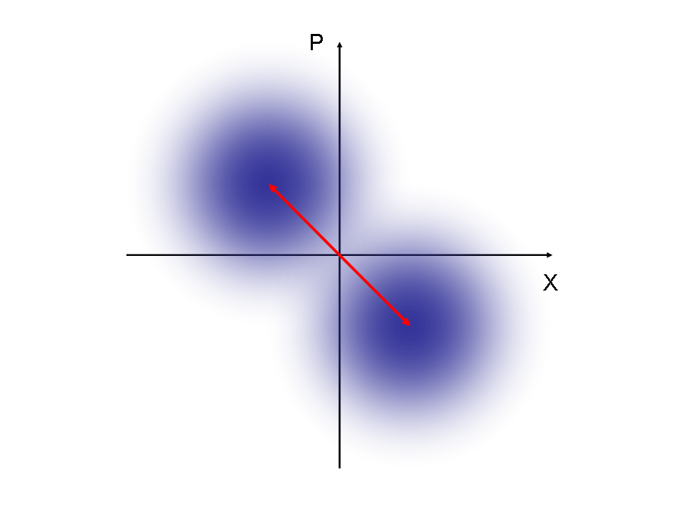
In any such protocol, Alice sends $n$ random coherent states drawn from either $\mathcal{S}_{2}=\{|\alpha e^{-i\pi/4}\rangle,|\alpha e^{3i\pi/4}\rangle\}$ or $\mathcal{S}_{4}=\{|\alpha e^{i\pi/4}\rangle,|\alpha e^{3i\pi/4}\rangle,|\alpha e^{5i\pi/4}\rangle,|\alpha e^{7i\pi/4}\rangle\}$ where $\alpha$ is chosen to be a positive real number. Then, for each state, Bob performs an homodyne measurement on a random quadrature $x$ or $p$. Note that in the case of the two-state protocol, Bob’s measurement is not the optimal measurement to distinguish between the state $|\alpha e^{-i\pi/4}\rangle$ and $|-\alpha e^{-i\pi/4}\rangle$. For both protocols, Bob obtains the real random variable $y_{i}$ for $i\in\{1,\cdots,n\}$. Alice and Bob use a reverse reconciliation, and the sign $b_{i}$ of $y_{i}$ encodes the raw key bit: we note $b_{i}=1$ if $y_{i}\geq 0$ and $b_{i}=0$ if $y_{i}<0$. Alice must then recover the value of the string ${\bf b}=(b_{1},\cdots,b_{n})$. To help her, Bob sends some side-information consisting of the quadrature measured, $x$ or $p$, the absolute value of $y_{i}$ for $i\in\{1,\cdots,n\}$ as well as the syndrome of ${\bf b}$ for a linear error correcting code Alice and Bob agreed on beforehand. Alice then proceeds by decoding her word ${\bf x}=\{x_{1},\cdots,x_{n}\}$ where $x_{i}$ corresponds to the sign of the quadrature Bob measured for the state she sent. An alternative protocol for the four-state protocol consists for Bob to perform an heterodyne (instead of homodyne) measurement [23, 24]. In this case, he measures both quadratures, and obtains two measurement results $y_{i}^{x}$ and $y_{i}^{p}$ for each state sent by Alice. The raw key now consists of both signs of $y_{i}^{x}$ and $y_{i}^{p}$.

As usual in all QKD schemes, a supplementary step has to be added for channel estimation: Alice and Bob reveal a fraction of their data and compute the covariance matrix of the state $\rho_{AB}$ that they would share in an entanglement-based version of the protocol [25]. This allows them to compute an upper bound on Eve’s information on $y$, the Holevo information $S(y;E)$. If the error correcting code used by Alice and Bob has a rate $R$, the secret key rate against collective attacks (in the limit where the fraction of data revealed for parameter estimation becomes negligible) reads:

$R$ is upper bounded by the mutual information $I(x;y)$ between Alice and Bob and one can therefore introduce the reconciliation efficiency $\beta$ defined as $\beta=R/I(x;y)$. One then finds the more common expression for the secret key rate:

With this expression, it is clear that being able to perform an efficient reconciliation, with $\beta$ close enough to 1, is crucial. Unfortunately, for a Gaussian modulation, the best reconciliation schemes [26, 14] presently known see their efficiency drop under $50\%$ at low signal to noise ratios (SNR). This is rather dramatic in terms of the range of the protocol as one needs to work at low SNR to distribute secret over long distances. A hand waving argument for this fact is given now. It is known [27, 28] that the quantity $K_{\mathrm{perf}}=I(x;y)-S(y;E)$ tends to a finite limit as the modulation variance $V_{A}$ of Alice tends to infinity. However, both quantities $I(x;y)$ and $S(y;E)$ diverge to infinity. As a consequence, the penalty $(1-\beta)I(x;y)$ imposed by an imperfect reconciliation also goes to infinity for any value of $\beta$ stricly less than 1. Therefore, one should not work with a large modulation variance as soon as the reconciliation is not perfect, which is never the case. On the contrary, for a realistic reconciliation efficiency (around $80\%$), the optimal modulation variance is typically quite low (less than 10 photons per pulse on average). Associated with high loss channels, i.e. long distance, the SNR is finally very low, well below 1 and reconciliation schemes for Gaussian modulation fail, meaning that no secret key can be exchanged over long distances with such a scheme.

An appealing alternative appears with discrete modulation schemes. The reason for this is that good reconciliation procedures can be found, even at very low SNR, for some modulation schemes. More precisely, in the case of the BI-AWGN channel (where Alice uses a binary modulation $\pm\alpha$ on an AWGN channel), good error correction codes are known at very low SNR [15]. Such a binary modulation scheme for error correction can be implemented either with a two-state protocol with coherent states in $\mathcal{S}_{2}$ or a four-state protocol with coherent states in $\mathcal{S}_{4}$. In particular, the error correcting codes presented in [15] allow one to get a reconciliation efficiency of $80\%$ for arbitrary low SNR. The main drawback of such protocols is that the methods used to upper bound $S(y;E)$ in the protocol using a Gaussian modulation [4, 5, 6] cannot be directly applied in the case of a discrete modulation scheme. One then needs to come up with a security proof specific to such protocols. We address this question in the next section.

In the remaining of the document, we use the notation $\gamma=\alpha e^{7i\pi/4}=\alpha e^{-i\pi/4}$ so that the set $\mathcal{S}_{2}$ of coherent states used in the two-state protocol is $\{|\gamma\rangle,|-\gamma\rangle\}$.

The security of the various protocols we consider here is studied through entanglement-based versions of the protocols. In the prepare and measure version of the protocols that are used in practice, Alice randomly draws $n$ binary or quaternary variables, each corresponding to a specific coherent state of $\mathcal{S}_{2}$ for the two-state protocol or of $\mathcal{S}_{4}$ in the case of the four-state protocol. Alice then prepares these $n$ coherent states and sends them to Bob through the quantum channel. In the entanglement-based version of the protocol, Alice starts with a pure bipartite state $|\Phi_{2}\rangle$ (or $|\Phi_{4}\rangle$, depending on the protocol) and performs a projective measurement on the first half of this state. The second half is sent to Bob through the quantum channel. For instance, in the protocol with a Gaussian modulation [3], the initial bipartite state is a two-mode squeezed vacuum, and the projective measurement performed by Alice is an heterodyne measurement, which projects the second half of the state on a coherent state [25]. The covariance matrix $\Gamma_{\mathrm{TMS}}$ of the two-mode squeezed vacuum reads

where $\sigma_{z}=\left(\begin{array}[]{cc}1&0\\ 0&-1\end{array}\right)$ and $Z_{G}=2\sqrt{\alpha^{4}+\alpha^{2}}$. Rewriting $\Gamma_{\mathrm{TMS}}$ with a direct reference to Alice’s modulation variance $V_{A}$ in the prepare and measure protocol, one has:

As the second half of the state is sent through a quantum channel characterized by its transmission $T$ and excess noise $\xi$, one can write the covariance matrix $\Gamma_{G}$ of the state $\rho_{AB}$ Alice and Bob share in the CV QKD protocol with a Gaussian modulation:

Then the Holevo information between Eve and Bob’s measurement result can be upper bounded by a function of $\Gamma_{G}$ [5]. Note indeed that the argumentation in [5] does no rely on the fact that the state considered is indeed Gaussian: only the covariance matrix of the states matters. This is not the case in [4] and [6] where the proof technique explicitely requires the modulation to be Gaussian.

For the protocols of interest in this article, the goal is to apply the same type of proof technique. We therefore want to find a purification $|\Phi_{2}\rangle$ (resp. $|\Phi_{4}\rangle$) with a covariance matrix $\Gamma_{2}$ (resp. $\Gamma_{4}$) as close as possible as the one of a two-mode squeezed state. This covariance matrix has the following form:

and the goal is to find a bipartite state $|\Phi_{2}\rangle$ (resp. $|\Phi_{4}\rangle$) such that $Z_{2}$ (resp. $Z_{4}$) is as close as possible of $Z_{G}$. Of course, in order to be a legitimate entanglement-based version of the protocol, the bipartite initial state must be such that there exists a projective measurement that Alice can perform that projects the second half of the state onto the desired 2 (or 4) coherent states of the set $\mathcal{S}_{2}$ (or $\mathcal{S}_{4}$). Also, it is worth emphasizing that, while the security proof of the Gaussian protocol is based on (virtual) Gaussian entanglement, the present proof is based on (virtual) non-Gaussian entanglement, which appears in this context as a convenient theoretical tool.

Now, the main idea of the discrete modulation protocols we study here is that there exists a regime for the modulation variance, $V_{A}$, such that

but with $\beta_{2}\approx\beta_{4}\gg\beta_{G}$. Here, the various subscripts $2,4,G$ refer to the different protocols: the binary modulation, the quaternary modulation and the Gaussian modulation. The existence of this regime allows one to have $K_{2},K_{4}>0$ for distances where the secret key rate for a Gaussian modulation $K_{G}$ is null.

The next two sections are concerned with the study of such states $|\Phi_{2}\rangle$ and$|\Phi_{4}\rangle$ and computing the correlation terms $Z_{2}$ and $Z_{4}$ of their covariance matrices.

We introduce a new QKD protocol involving two coherent state $\{|\alpha e^{-i\pi/4}\rangle,|-\alpha e^{-i\pi/4}\rangle\}$ where the detection is an homodyne measurement on a randomly chosen quadrature $x$ or $p$. This protocol is quite similar to the protocol studied in [22] but the difference between the two protocols is that in [22], the two coherent states are modulated along one of the quadratures measured by Bob. This is not the case here. The security analysis follows the same lines as for the recently introduced four-state protocol [15].

In the prepare and measure version of the protocol, Alice sends the coherent states $\{|\gamma\rangle$ and $|-\gamma\rangle\}$ with probability $1/2$ to Bob. Hence Bob sees a mixture $\rho_{2}$ given by:

where $\mu_{0}=e^{-\alpha^{2}}\cosh{\alpha^{2}}$, $\mu_{1}=e^{-\alpha^{2}}\sinh{\alpha^{2}}$ and

In order to use the proof technique described in the previous section, we need to consider the entanglement based version on the protocol. In this version, Alice starts with a bipartite non-Gaussian pure state $|\Phi_{2}\rangle$. She performs a projective measurement on one half of the state and sends the other half to Bob through the quantum channel. Depending on the binary result of her measurement, the state sent to Bob is either $|\gamma\rangle$ or $|-\gamma\rangle$ with equal probabilities. Let us consider the following purification for $\rho$:

where $|\phi_{0}^{*}\rangle$ and $|\phi_{1}^{*}\rangle$ are simply defined as:

where we recall that $\alpha$ is a positive number. $|\Phi_{2}\rangle$ can also be rewritten as:

with

At this point, it is worth noting that in the entanglement based version of the protocol, Alice simply applies the projective measurement $\{|\psi_{0}\rangle\langle\psi_{0}|,|\psi_{1}\rangle\langle\psi_{1}|\}$ to the first half of the state $|\Phi_{2}\rangle$ and that she therefore projects the second half either on the coherent state $|\gamma\rangle$ or the coherent state $|-\gamma\rangle$ with equal probabilities. The Wigner functions of the orthogonal non-Gaussian states $|\psi_{0}\rangle$ and $|\psi_{1}\rangle$ corresponding to Alice’s projective measurement are displayed on Figure 2. Note that $|\psi_{0}\rangle$ is peaked close to the coherent state $|\alpha e^{i\pi/4}\rangle$ while $|\psi_{1}\rangle$ is peaked close to $|\alpha e^{5i\pi/4}\rangle$.

We now proceed with evaluating the covariance matrix $\Gamma_{2}$ of $|\Phi_{2}\rangle$. Straightforward algebraic manipulations show that it has the following form:

with

where $a,a^{\dagger}$ and $b,b^{\dagger}$ are respectively the annihilation and creation operators on Alice and Bob’s modes of the state.

In order to compute $X$, one can consider the state $\rho_{A}=\frac{1}{2}\left(|\gamma^{*}\rangle\langle\gamma^{*}|+|-\gamma^{*}\rangle\langle-\gamma^{*}|\right)$ obtained by tracing over the second subsystem of $|\Phi_{2}\rangle$:

since $a|\pm\gamma\rangle=\pm\gamma\;|\pm\gamma\rangle$. The symmetry of the state $|\Phi_{2}\rangle$ shows that

One easily notes that

and

Hence, applying the operator $ab$ on the state $|\Phi_{2}\rangle$ gives:

and:

and finally

The quantity $Z_{2}$ is displayed on Figure 4. For a variance of modulation less than $0.05$, that is $\alpha\lessapprox 0.15$, $Z_{2}$ is almost indistinguishable from $Z_{G}$ thus suggesting that in this regime, $S_{2}(y;E)\approx S_{G}(y;E)$. This behaviour will be confirmed in Section 7.

In this section, we study the protocol recently introduced in [15]. More specifically, we introduce a non-Gaussian state $|\Phi_{4}\rangle$ that can be used in an entanglement-based version of the protocol and for which we compute the covariance matrix.

In the prepare and measure version of the protocol, Alice sends the coherent states $\{|\gamma\rangle,|\gamma^{*}\rangle,|-\gamma\rangle$ and $|-\gamma^{*}\rangle\}$ with probability $1/4$ to Bob. Hence Bob sees a mixture $\rho_{4}$ given by:

where

and

for $k\in\{0,1,2,3\}$.

Applying the annihilation operator $a$ to $|\phi_{k}\rangle$ gives:

for $k\in\{1,2,3\}$ and

Let us now introduce the following purification $|\Phi_{4}\rangle$ of the state $\rho_{4}$:

This state can also be written as:

where the states

are orthogonal non-Gaussian states. These states are displayed on Figure 3.

In the entanglement-based version of the protocol, Alice needs to perform a projective measurement having these states as eigenstates, in order to project the second half of $|\Phi_{4}\rangle$ on one of the four coherent states of $\mathcal{S}_{4}$, namely $\{|\psi_{0}\rangle\langle\psi_{0}|,|\psi_{1}\rangle\langle\psi_{1}|,|\psi_{2}\rangle\langle\psi_{2}|,|\psi_{3}\rangle\langle\psi_{3}|\}$.

Let us compute the covariance matrix $\Gamma_{4}$ of the bipartite state $|\Phi_{4}\rangle$. One can show that $\Gamma_{4}$ has the following form:

where

We are now interested in the correlation term of the covariance matrix, that is

One has:

where addition should be understood modulo 4. Finally, we obtain:

The behaviour of $Z_{4}$ is plotted on Figure 4. For $V_{A}\lessapprox 0.5$, that is $\alpha\lessapprox 0.5$, $Z_{4}$ and $Z_{G}$ are almost indistinguishable, meaning that in this regime, one has $S_{4}(y;E)\approx S_{G}(y;E)$. We confirm this intuition in the next section.

For both protocols, the Holevo information between Eve and Bob’s measurement result is upper bounded by the same quantity computed for a Gaussian state $\rho^{G}_{AB}$ with the same covariance matrix as the state $\rho_{AB}$ shared by Alice and Bob in an entanglement-based version of the protocol. Hence one can give a lower bound for both secret key rates $K_{2}$ and $K_{4}$:

The expression for the upper bound on $S_{2}(y;E)$ (resp. $S_{4}(y;E)$) is computed from the symplectic eigenvalues $\nu_{1},\nu_{2}$ of $\Gamma_{2}$ (resp. $\Gamma_{4}$) and from the eigenvalue $\nu_{3}$ of the matrix $\Gamma_{2}^{\mathrm{hom}}$ (resp. $\Gamma_{4}^{\mathrm{hom}}$ or $\Gamma_{4}^{\mathrm{het}}$ depending on the nature of the measurement ) corresponding to the covariance matrix of Alice’s state given the result $y$ of Bob’s homodyne (or heterodyne) measurement [8].

We computed in the previous sections the covariance matrix of the bipartite state prepared by Alice, that is, before the quantum channel. In order to bound Eve’s information, we need to know the covariance matrix $\Gamma_{2,4}$ of the state shared by Alice and Bob, that is, after the quantum channel.

In this paper, we make the assumption that the quantum channel is linear (see A for details). In that case, one can easily use standard techniques from statistics (see Ref. [29]) in order to estimate its transmission $T$ and excess noise $\xi$.

The covariance matrix $\Gamma_{2,4}$ of the state shared by Alice and Bob is given by:

The reduced covariance matrix given Bob’s measurement result depends on the type of measurement performed, either homodyne or heterodyne:

and

Let us now explain how these covariance matrices can be estimated from experimental data. Indeed, one should recall that these covariance matrices correspond to a virtual bipartite state, namely the state that Alice and Bob would share in the entanglement-based version of the protocol. Therefore, they cannot be measured directly. Let us note $x$ and $y$ the respective random variables corresponding to Alice and Bob’s classical data in the prepare and measure scenario. One can show that the covariance matrices above can be derived from the observed second moments of the variables $x$ and $y$, that is $\langle x^{2}\rangle,\langle xy\rangle$ and $\langle y^{2}\rangle$. One has: $V_{A}=\langle x^{2}\rangle$, $T=\frac{\langle xy\rangle^{2}}{\langle x^{2}\rangle^{2}}$ and $TV_{A}+2+T\xi=\langle y^{2}\rangle$.

This shows that the covariance matrices in the entanglement-based scenario are indeed accessible from the experimental data in the actual prepare and measure protocol, assuming that the quantum channel is linear.

First, it is worth mentioning that the bounds for the Holevo information $S(y;E)$ that we derive from the covariance matrices of $|\Phi_{2}\rangle$ and $|\Phi_{4}\rangle$ are not proven to be tight. Indeed, even in the case where the quantum channel between Alice and Bob is perfect, that is, $T=1$ and $\xi=0$, the bounds we compute do not give $S(b;E)=0$ as we would expect, except in the limit of infinitely small modulation variances $\alpha\rightarrow 0$. This is because the states $|\Phi_{2}\rangle$ and $|\Phi_{4}\rangle$ are not Gaussian. However, the approximation becomes reasonably good for low modulation variances and one can expect the bounds not to be too loose. An intriguing question is whether the value of $S(y;E)$ computed for the Gaussian protocol is an upper bound for the same quantity computed for the discrete-modulation protocols. With the proof we presented, this is not the case (for instance, for a perfect quantum channel, $S_{G}(y;E)=0$ as expected, whereas the bounds we found for $S_{2}(y;E)$ and $S_{4}(y;E)$ are positive). It is quite natural to expect the following relation to hold $S_{2}(y;E),S_{4}(y;E)<S_{G}(y;E)$ since a discrete modulation never maximizes the mutual information between Alice and Bob, and it is doubtful that it presents any advantage for a eavesdropper. However, our security proof cannot bring a definitive answer to this question.

The performances of the two-state protocol are displayed on Figure 5 corresponding to a realistic scheme where the reconciliation efficiency is only $80\%$ and the quantum efficiency of Bob’s detector is equal to $60\%$ (these values are compatible with state-of-the-art experimental implementations [9]).

One can see from Figure 5 that the two-state protocol can only work in a regime where the excess noise is very small: around $1/1000$. We note that this result is compatible with the results obtained in [22] where the authors study the security of a slightly different version of the two-state protocol, where they need to assume the perfect knowledge of the probability distribution $p(y|x)$ of Bob’s measurements results given Alice’s results.

The performance of the four-state protocol with a homodyne detection is presented on Figure 6 for an realistic reconciliation efficiency of $80\%$ as well as a realistic quantum efficiency of $60\%$ for Bob’s detector (which is treated as part of the overall loss between Alice and Bob). The performance of the protocol with a heterodyne detection is displayed on Figure 7. One immediately notices that the four-state protocol performs much better than its two-state counterpart, that is, it allows for a distribution of secret keys over longer distances, and tolerates a much higher (and more reasonable) excess noise. Note that choosing a homodyne or a heterodyne detection does not sensibly affect the performances of the protocol. The better resistance to excess noise of these protocols is extremely important because the results presented so far are a little too optimistic, in the sense that they assume a perfect knowledge of the transmission and excess noise (which is already infinitely less demanding that requiring a perfect knowledge of the quantum channel, which is described by an infinite number of parameters). In practice, however, these parameters can never be perfectly known, and they can only be estimated with a precision depending on the number $N-n$ of data used in the parameter estimation. The main consequence of this imperfect parameter estimation is to increase the effective excess noise, thus decreasing the actual performance of the protocols. The finite size effects for CV QKD protocols are investigated elsewhere [29].

We introduced continuous-variable quantum key distribution protocols displaying a discrete modulation. We consider the cases of two and four state modulation. We established the security of these protocols against collective attacks for which the quantum channel is linear. As expected, the four-state protocol clearly outperforms the two-state protocol. The generalization to modulation schemes with a higher number of states may be considered, but it is not so straightforward as one would lose the main advantage of the protocols presented here, that is, their very efficient reconciliation procedure. However, if one allows for a heterodyne detection instead of a homodyne detection, new continuous modulation schemes can lead to better performances [31].

An important question at that stage is how to avoid the extra hypothesis that the channel should be linear. As shown in Ref. [32], this can be done by using decoy states, in order to embed the non-Gaussian modulation into an overall gaussian modulation. It is then safe to evaluate the values of $T$ and $\xi$ from a gaussian probe beam, and then to use them as described in the present paper.

This work received financial support from Agence Nationale de la Recherche under projects PROSPIQ (ANR-06-NANO-041-05) and SEQURE (ANR-07-SESU-011-01).

References

- [1] Scarani V, Bechmann-Pasquinucci H, Cerf N J, Dušek M, Lütkenhaus N and Peev M 2009 Rev. Mod. Phys. 81 1301
- [2] Bennett C H and Brassard G 1984 Proc. IEEE Int. Conf. on Computers, Systems and Signal Processing 175
- [3] Grosshans F and Grangier P 2002 Phys. Rev. Lett. 88 057902
- [4] Navascués M, Grosshans F and Acín A 2006 Phys. Rev. Lett. 97 190502
- [5] García-Patrón R and Cerf N J 2006 Phys. Rev. Lett. 97 190503
- [6] Leverrier A and Grangier P 2009 arXiv 0912.4132
- [7] Renner R and Cirac J I 2009 Phys. Rev. Lett. 102 110504
- [8] Lodewyck J, Bloch M, García-Patrón R, Fossier S, Karpov E, Diamanti E, Debuisschert T, Cerf N J, Tualle-Brouri R, McLaughlin S W and Grangier P 2007 Phys. Rev. A 76 042305
- [9] Fossier S, Diamanti E, Debuisschert T, Villing A, Tualle-Brouri R and Grangier P 2009 New J. Phys. 11 045023
- [10] Grosshans F and Grangier P 2002 arXiv quant-ph/0204127
- [11] Grosshans F, Van Assche G, Wenger J, Brouri R, Cerf N J and Grangier P 2003 Nature 421 238–241
- [12] Silberhorn Ch, Ralph T C, Lütkenhaus N and Leuchs G 2002 Phys. Rev. Lett. 89 167901
- [13] Heid M and Lütkenhaus N 2007 Phys. Rev. A 76 022313
- [14] Leverrier A, Alléaume R, Boutros J, Zémor G and Grangier P 2008 Phys. Rev. A 77 042325
- [15] Leverrier A and Grangier P 2009 Phys. Rev. Lett. 102 180504
- [16] Namiki R and Hirano T 2003 Phys. Rev. A 67 022308
- [17] Namiki R and Hirano T 2004 Phys. Rev. Lett. 92 117901
- [18] Lorenz S, Korolkova N and Leuchs G 2004 Appl. Phys. B 79 273
- [19] Namiki R and Hirano T 2006 Phys. Rev. A 74 032302
- [20] Heid M and Lütkenhaus N 2006 Phys. Rev. A 73 052316
- [21] Sych D and Leuchs G 2010 New J. Phys. 12 053019
- [22] Zhao Y, Heid M, Rigas J and Lütkenhaus N 2009 Phys. Rev. A 79 012307
- [23] Weedbrook C, Lance A M, Bowen W P, Symul T, Ralph T C and Lam P K 2004 Phys. Rev. Lett. 93 170504
- [24] Weedbrook C, Lance A M, Bowen W P, Symul T, Ralph T C and Lam P K 2006 Phys. Rev. A 73 022316
- [25] Grosshans F, Cerf N J, Wenger J, Tualle-Brouri R and Grangier P 2003 Quantum Information and Computation 3 535–552
- [26] Bloch M, Thangaraj A, McLaughlin S W and Merolla J M 2006 Proc. IEEE Information Theory Workshop 116-
- [27] Grosshans F 2005 Phys. Rev. Lett. 94 020504
- [28] Navascués M and Acín A 2005 Phys. Rev. Lett. 94 020505
- [29] Leverrier A, Grosshans F and Grangier P 2010 Phys. Rev. A 81 062343, see also Leverrier A 2009 PhD Dissertation http://tel.archives-ouvertes.fr/tel-00451021
- [30] Grangier P, Levenson J A and Poisat JP 1998 Nature 396 6711
- [31] Leverrier A, Grangier P 2010 arXiv:1005.0328
- [32] Leverrier A, Grangier P 2011 arXiv:1101.3008
- [33] Richardson T J, Shokrollahi M A and Urbanke R L 2001 IEEE Transactions on Information Theory 47 619–637
- [34] Richardson T and Urbanke R 2002 Workshop honoring Prof. Bob McEliece on his 60th birthday 24–25