Causal Markov condition for submodular information measures
Abstract
The causal Markov condition (CMC) is a postulate that links observations to causality. It describes the conditional independences among the observations that are entailed by a causal hypothesis in terms of a directed acyclic graph. In the conventional setting, the observations are random variables and the independence is a statistical one, i.e., the information content of observations is measured in terms of Shannon entropy. We formulate a generalized CMC for any kind of observations on which independence is defined via an arbitrary submodular information measure. Recently, this has been discussed for observations in terms of binary strings where information is understood in the sense of Kolmogorov complexity. Our approach enables us to find computable alternatives to Kolmogorov complexity, e.g., the length of a text after applying existing data compression schemes. We show that our CMC is justified if one restricts the attention to a class of causal mechanisms that is adapted to the respective information measure. Our justification is similar to deriving the statistical CMC from functional models of causality, where every variable is a deterministic function of its observed causes and an unobserved noise term.
Our experiments on real data demonstrate the performance of compression based causal inference.
1 Introduction
Explaining observations in the sense of inferring the underlying causal structure is among the most important challenges of scientific reasoning. In practical applications it is generally accepted that causal conclusions can be drawn from observing the influence of interventions. The more challenging task, however, is to infer causal relations on the basis of non-interventional observations and research in this direction still is considered with skepticism. It is therefore important to thoroughly formalize the assumptions and discuss the conditions under which they are satisfied. For causal reasoning from statistical data, Spirtes, Glymour, Scheines [1] and Pearl [2] formalized the assumptions under which the task is solvable. With respect to a causal hypothesis in terms of a directed acyclic graph (DAG) the most basic assumption is the causal Markov condition stating that every variable is conditionally independent of its non-descendants, given its parents,
for short. Pearl argues that this follows from a “functional model” of causality (or non-linear structure equations), where every node is a deterministic function of its parents and an unobserved noise term (see Fig. 1), i.e.,
| (1) |
The causal Markov condition is then a consequence of the statistical independence of the noise terms, which is called causal sufficiency. It can be justified by the assumption that every dependence between them requires a common cause (as postulated by Reichenbach [3]), which should then explicitly appear in the causal model. From a more abstract point of view, condition (1) can be interpreted as saying that the node does not add any more information that is not already contained in the parents and the noise together. If we restrict the assumption to discrete variables, the corresponding information measure can be, for instance, the Shannon entropy, but also other measures could make sense.
In [4] the probabilistic setting is generalized to the case where every observation is formalized by a
binary string (without any statistical population). The information content of an observation is then measured using
Kolmogorov complexity (also “algorithmic information”) which gives rise to an algorithmic version of (conditional) mutual information.
The corresponding functional model is given by a Turing machine that computes the string from its parent strings and a noise .
The algorithmic information theory based approach generalizes the statistical framework since the average algorithmic information content per instance of a sequence of i.i.d. observations converges to the Shannon entropy, but on the other hand observations need not be generated by i.i.d. sampling.
Unfortunately, Kolmogorov complexity is uncomputable and practical causal inference schemes must deal with other measures of information. In Section 2 we define general information measures and show that they induce independence relations that satisfy the semi-graphoid axioms (Section 3). Then, in Section 4, we phrase the causal Markov condition within our general setting and explore under which conditions
it is a reasonable postulate. To this end, we formulate an information theoretic version of functional models observing that their decisive feature is that the joint information of a node, its parents and its noise is the same as the joint information of its parents and noise alone. We demonstrate with examples how these functional models restrict the set of allowed causal mechanisms to a certain class (Section 5). We emphasize that the choice of the information measure determines this class and is therefore the essential prior decision
(which certainly requires domain knowledge). Thus, when applying our theory to real data, one first has to think about the causal mechanisms to be explored and then design an information measure that is sufficiently “powerful” to detect the generated dependences.
Section 6 discusses a modification for known independence based causal inference that is necessary for those information measures for which conditioning can only decrease dependences. Section 7 describes one of the most important intended applications of our theory, namely information measures based on compression schemes (e.g. Lempel-Ziv). Applications of these measures using the PC algorithm for causal inference to segments of English text demonstrate the strength of causal reasoning that goes beyond already known applications of compression for the purpose of (hierarchical) clustering.
2 General information measures
In this section we define information from an axiomatic point of view and prove properties that will be useful in the derivation of the causal Markov condition. We start by rephrasing the usual concept of measuring statistical dependences. Let be a set of discrete-valued random variables and be the set of subsets. For each let denote the joint Shannon entropy of the variables in . For three disjoint sets the conditional mutual information between and given then reads
| (2) |
The set of subsets constitutes a lattice with respect to the operations of union and intersection and can be seen as a function on this lattice11 1 Also the information function that are presented in this paper can all be rephrased as functions on the lattice of subsets it is nevertheless notationally convenient to formulate the theory with respect to general lattices.. We observe that the non-negativity of (2) can be guaranteed if
for two sets . This submodularity condition is known to be true for Shannon entropy [5]. Motivated by these remarks, we now introduce an abstract information measure defined on the elements of a general lattice. Throughout this paper let be a finite lattice and denote by the meet of all of its elements.
Definition 1 (information measure)
We say
is an information measure if it satisfies the following axioms:
(1) normalization:
(2) monotonicity: implies for all ,
(3) submodularity: for all .
Note that submodular functions have been considered in different contexts for example in [6] and [7].
Based on we define a conditional version for all by
For ease of notation we write instead of . In analogy to (2), gives rise to the following measure of independence.
Definition 2 (conditional mutual information)
For the conditional mutual information of and given is defined by
We say and are independent given or equivalently if .
The following Lemmas generalize usual information theory.
Lemma 1 (non-negativity of mutual information and conditioning)
For we have
Proof: By definition, is equivalent to . Defining and and using associativity of we have . Further, using Lemma 4 in Ch.1 from [8], in any lattice
and hence by monotonicity of : . Combining everything
where the first inequality uses submodularity of .
The first inequality follows from by . The second inequality follows directly from and the definition of .
Lemma 2 (chain rule for mutual information)
For
| (3) |
Proof: This is directly seen by using the definition of conditional mutual information on both sides.
Lemma 3 (data processing inequality)
Given it holds
Proof: The first implication is clear. For the second we apply the chain rule for mutual information two times and obtain
since the second summand is zero by assumption and conditional mutual information is non-negative.
3 Submodular dependence measures and semi-graphoid axioms
The axiomatic approach to stochastic independence goes back to Dawid [9] who stated four axioms of conditional independence that are fulfilled for any kind of probability distribution. Later, any relation on triplets that satisfies the same axioms has been named semi-graphoid in [2]. In the following we show that the function constructed from in the last section satisfies these axioms.
Lemma 4 ( satisfies semi-graphoid axioms)
The function defined in the last section satisfies the semi-graphoid axioms, namely for
Proof: Symmetry is clear and the remaining implications follow directly from the chain rule and non-negativity.
On the contrary, if we are given a function , what axioms do we need to define a submodular information measure from ? It turns out that the chain rule in eq. (3) together with non-negativity and symmetry already implies that is an information measure and coincides with the dependence measure introduced in Definition 2. We omit the proof due to space constraints.
Thus we characterized the type of dependence measures that we are able to incorporate into our framework. To show that the chain rule is actually a strong restriction we close the section with an example of independence of orthogonal linear subspaces.
Example: (orthogonal subspaces, qualitative version e.g. in [10])
Linear subspaces of some finite vector space form a lattice, where the union of two subspaces is the subspace generated by the set-theoretic union. For two such subspaces and write for the orthogonal projection of onto . We define , hence orthogonal subspaces are considered as independent. Given a third subspace the conditional version reads
where and denote the orthogonal projections of and to the orthogonal complement of . is symmetric and non-negative, but it does not satisfy the chain rule. This is because projecting a subspace first to and then to is different from projecting it to . Hence we can not find a submodular function underlying our dependence measure. Nevertheless satisfies the semi-graphoid axioms and can thus be considered as a measure of independence.
4 Causal Markov condition for general information measures
In this section we define three versions of the causal Markov condition with respect to a general submodular information measure and show that they are equivalent (similar to the statistical framework). Then we discuss under which conditions we expect it to be a reasonable postulate that links observations with causality. Assume we are given observations that are connected by a DAG. It is no restriction to consider the observations as elements of a lattice, e.g. the lattice of their subsets.
Definition 3 (causal Markov condition (CMC), local version)
Let be a that describes the causal relations among observations . Then the observations are said to fulfill the causal Markov condition with respect to the dependence measure if
where denotes the join of the parents of and the join of its non-descendants (excluding the parents).
The intuitive meaning of the postulate is that conditioning on the direct causes of an observation screens off its dependences from all its non-effects. The following theorem generalizes results in [10] for statistical independences and [4] for algorithmic independences. In particular it states that if the causal Markov condition holds with respect to a graph , then independence relations implied by the CMC can be obtained through the convenient graph-theoretical criterion of -separation ([2], [1]).
Theorem 1 (Equivalence of Markov conditions and information decomposition)
Let the nodes of a DAG be
elements of some lattice and be
an information measure on . Then the following three properties are equivalent
- (1)
fulfill the (local) causal Markov condition.
- (2)
For every ancestral set22 2 A set of nodes of a DAG G is called ancestral, if for every the parents of are in too. , decomposes according to :
- (3)
The global Markov condition holds, i.e., if three sets of nodes are d-separated in , then
The proof is provided in Appendix A. The second condition shows that the joint information of observations can be recursively computed according to the causal structure. The third condition describes explicitly which sets of independences are implications of the causal Markov condition.
Our next Theorem will show that the CMC follows from a general notion of a functional model. At its basis is the following Lemma describing that the CMC on a given set of observations can be derived from the causal Markov condition with respect to an extended causal graph (see Figure 1).
Lemma 5 (causal Markov condition from extended graph)
Let the nodes of a DAG be elements of a lattice with an independence relation that is monotone and satisfies the chain rule. If there exist additional elements such that for all
| (4) |
and the are jointly independent in the sense that
| (5) |
then the fulfill the causal Markov condition with respect to .
Proof: Based on we construct a new graph with node set and an additional edge for every . We first show that the causal Markov condition holds for the nodes of : By construction, the join of non-descendants of with respect to is equal to . Since the join of the parents of in are , assumption (4) just states which is the local CMC with respect to . To see that CMC also holds for , observe that the non-descendants of are equal to the non-descendants of in and since does not have any parents, we have to show
| (6) |
Using together with the chain rule for mutual information we get
where the last equality follows from (5). Let be the set of non-descendants of in . Note that is ancestral, that is if , then so are the ancestors of . We introduce a topological order on , such that if there is an edge in , then . Using the chain rule for mutual information iteratively we get
where denotes the join of elements of smaller than . By choice of our ordering the mutual information of and is conditioned at least on its parents and we can write , where is the join of elements smaller than in that are not its parents. Therefore, again by the chain rule, each summand on the right hand side can be bounded from above by writing
where the second inequality is true because by construction is the join of non-descents of . The right hand side vanishes because of assumption (4). This proves (6) and therefore the causal Markov condition with respect to .
By Theorem 1, -separation on implies independence. Due to the special structure of one can check that -separation in implies -separation in the extended graph . Again by Theorem 1, -separation implies the causal Markov condition for , which proves the lemma.
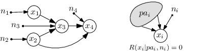
Now we formalize the intuition that in a generalized functional model a node only contains information that is already contained in the direct causes and the noise together (see Figure 1):
Definition 4 (functional model)
Let be a DAG with nodes in the lattice . If there exists an additional node for each , such that the are jointly independent and
| (7) |
then together with is called a functional model of the .
If we restrict our attention to causal mechanism of the above form, the CMC is justified:
Theorem 2 (functional model implies CMC)
If there exists a functional model for the nodes of a DAG then they fulfill the causal Markov condition with respect to .
Proof: In the functional model with noise nodes it holds for all . This implies . Since the in a functional model are assumed to be jointly independent, Lemma 5 can be applied and proves the theorem.
The following section describes examples of causal mechanisms that can be seen as functional models with respect to various information measures.
5 Examples of information measures and their functional models
Let be a finite set of observations which are in a canonical way elements of the lattice of subsets . Let the causal structure be a DAG with as nodes.
5.1 Shannon entropy of random variables
Let the be discrete random variables with joint probability mass function . For a subset denote by the random variable with distribution . The Shannon entropy for the subset is defined as . Monotony as well as submodularity are well-known properties [5]. The corresponding notion of independence is the familiar (conditional) stochastic independence, its information-theoretic quantification being mutual information. Then is equivalent to the existence of some function with
This restricts the set of mechanisms to those which were deterministic if one could take all latent factors into account. Note that continuous Shannon entropy is not monotone under restriction to subsets. Nevertheless, in this case the chain rule and non-negativity is true and therefore the CMC can be motivated by independences with respect to an extended causal model (Lemma 5 of the previous section).
5.2 Kolmogorov complexity of binary strings
Let the be binary strings and the information measure be the Kolmogorov complexity as information measure. More explicitly, for a subset of strings denote by a concatenation of the strings in a prefix free manner (which guarantees that the concatenation can be uniquely decoded into its components). The Kolmogorov complexity is then defined as the length of the shortest program that generates the concatenated string on a universal prefix-free Turing machine. It is submodular up to a logarithmic constant [11]. For two strings the conditional Kolmogorov complexity of , given is defined as the length of the shortest program that computes from the input . It must be distinguished from , the length of the shortest program that computes from the shortest compression of . Note that defining implies that the conditional information reads due to
see [12]. Then
which, in turn, is equivalent to the existence of a program of length that computes from the shortest compression of . Here we have considered the number of nodes as a constant, which ensures that the order of the strings does not matter. Such an “algorithmic model of causality”[4] restricts causal influences to computable ones. Uncomputable mechanisms can easily be defined (halting problem). However, in the spirit of the Church-Turing thesis, we will assume that they don’t exist in nature and conjecture that the algorithmic model of causality is the most general model of a causal mechanism as long as we restrict the attention to the non-quantum world (where the model would probably be replaced with a quantum Turing machine).
5.3 Period length of time series
We start with the following abstract example to illustrate that the definition of an information measure is more natural when the observations are taken to be part of a lattice different from the lattice of subsets. Let every observation be a natural number and consider them elements of the lattice of natural numbers where denotes the least common multiple and the greatest common divisor, hence for
We define an information measure by
Non-negativity and monotonicity of are clear and submodularity even holds with equality: For
The corresponding conditional dependence measure reads
so and are independent given if contains all prime factors that are shared by and (with at least the same multiplicity).
We define a functional model where every node contains only
prime factors that are already contained in its parents and its noise node (with at least the same multiplicity) and the noise terms are assumed to be relatively prime.
Such a lattice of observations can occur in real-life if denotes the period length of a periodic time series over . Then the period length of the joint time series defined by a set of nodes is obviously the least common multiple. If every time series at node is a function of its parents and noise node (each being a time series) and is time-covariant, divides their period lengths.
Assuming that the period lengths of the noise time series are relatively prime is indeed a strong restriction, but if we assume that the periods are large numbers and interpret independence in the approximate sense
we obtain the condition that their periods have no large factors in common. This seems to be a reasonable assumption if the noise time series have no common cause.
One can easily think of generalizations where every observation is characterized by a symmetry group and the join of nodes by the group intersection describing the joint symmetry. One may then define functional models where every node inherits all those symmetries that are shared by all its parents and the noise node.
5.4 Size of vocabulary in a text
Let every observation be a text and for every collection of texts let be the number of different meaningful words in . Here, meaningful means that we ignore words like articles and prepositions. To see that is submodular we observe that it is just the number of elements of a set.
We can use to explore which author has copied parts of the texts written by other authors: Let every be written by another author and a causal arrow from to means that the author of was influenced by when writing .
The noise can be interpreted as the set of words the author usually uses and the condition then means that he/she combines only words from the texts he/she has seen with the own vocabulary.
To conclude this section we want to emphasize that the above example refers to a dependence measure that is non-increasing under conditioning, that is for collections and of texts whenever . This is because is equal to the number of meaningful words contained in and , but not in . In general, the above information measure can be viewed as rank or height function (cardinality) on the lattice of sets of meaningful words and it can be shown that dependence measures originating form information functions that are rank functions on distributive lattices are always non-increasing under conditioning 33 3 Lattices with a rank function that is submodular are generally called semimodular lattices. Abstract independence measures on semimodular lattices have also been discussed in a different context by Cuzzolin [13].. We will elaborate on this point in the next section because it imposes special challenges for causal inference.
6 Faithfulness for monotone dependence measures
Apart from the CMC, the essential postulate of independence based causal inference is usually causal faithfulness. It states that all observed independence relations are structural, that is, they are induced by the true causal DAG through -separation. This postulate allows the identification of causal DAGs up to “Markov equivalence classes” imposing the same independences.
Faithfulness has already been defined for abstract conditional independence statements and we start by rephrasing the definition following ([1], p.81).
Definition 5 (faithfulness)
A DAG is said to represent a list of conditional independence relations on a set of observations faithfully, if consists exactly of the independence relations implied by through -separation. Further, a set of observations is said to be faithful (w.r.t. a given dependence measure), if there exists a causal model that represents faithfully.
The above definition of faithfulness makes sense for the probabilistic and algorithmic notions of dependence, but there is a problem with respect to dependence measures on which conditioning can only decrease information. As mentioned above, rank functions of distributive lattices lead to this kind of dependence measures, that we will call monotone in the following. To see the problem, consider for three observations a causal model of the form . By -separation, is independent of and for a monotone dependence measure this implies , which is not an independence induced by -separation. Hence, does not faithfully represent the objects and one can easily check that a faithful representation does not exist (e.g. using the theorem below). However, we can modify faithfulness such that it also accounts for those independences that follow from monotony under conditioning:
Definition 6 (monotone faithfulness)
A DAG is said to represent a list of conditional independences of observations monotonely faithful, if the following condition is true for all disjoint subsets whose join is denoted by and : Whenever is in and is minimal among all the sets that render and independent, then and are -separated by in . Further, a set of observations is said to be monotonely faithful (w.r.t. a given dependence measure), if there exists a causal model that represents monotonely faithful.
Note that, trivially, every faithful representation is a monotonely faithful representation, hence faithful observations are monotonely faithful observations. Faithful representations have already been characterized (Theorem 3.4 in [1]) and we prove an equivalent characterization that holds simultaneously for monotonely faithful and for faithful observations.
Theorem 3 (characterization of monotonely faithful representations)
A set of (monotonely) faithful observations is represented (monotonely) faithfully by a DAG if and only if
- (1)
two observations and are adjacent in if and only if they can not be made independent by conditioning on any join of observations in .
- (2)
for three observations , such that is adjacent to , is adjacent to and is not adjacent to , it holds that in if and only if there exists a set such that is independent of given the join of the observations in .
The proof is given in the appendix.
The theorem implies in particular, that every monotonely faithful representation of faithful objects is already a faithful representation.
The PC algorithm [14, 1] for causal inference takes a set of conditional independences on faithful objects and returns the equivalence class of faithful representations. Since the above theorem is used to prove the correctness of the algorithm in the faithful case, we conclude that the algorithm correctly returns monotonely faithful representations given monotonely faithful observations. We apply the PC-algorithm with respect to compression based information functions in the following section. Also they are not monotone in a strict theoretical sense, empirical observations indicate that it is unlikely for the mutual information to increase.
7 Compression based information
In this section we demonstrate that our framework enables us to do causal inference on single objects (coded as binary strings) without relying on the uncomputable measure of Kolmogorov complexity. To this end, instead of defining complexity with respect to a universal Turing machine we explicitly limit ourselves to specific production processes of strings. The underlying measure of information is motivated by universal compression algorithms like LZ77 [15] and grammar based compression [16] that detect repeated occurrences of identical substrings within a given input string and encode them more efficiently. The choice of a compression scheme can be seen as a prior analogously to the choice of a universal Turing machine in the case of algorithmic information. The measures considered in this section quantifiy the information of an observation (string) in terms of the diversity of its substrings and entail the following assumption on causal processes: A mechanism that produces a string from a string is considered as simple, if it constructs by concatenating a small number of substrings from (see Lemma 7 below for a formal statement). Further, the amount of dependence of observations is approximately given by the number of substrings that they share.
We are going to describe two specific measures of information that are closely related to the total length of the compressed string, but have better formal properties than the latter. This way our conclusions will be independent of the actual implementation of the compression scheme and proving theoretical results gets easier.
In the last part of this section we describe experiments on real data in which the PC algorithm is applied to infer the causal structure using either of the two introduced measures of information.
Note that distance metrics based on compression length have already been used to cluster various kinds of data (see [17] for computable distance metrics motivated by algorithmic mutual information or [18] for an application to molecular biology). These metrics can be used to reconstruct trees (hierarchical clustering) but if two nodes are linked by more than one path a measure of conditional mutual information is needed to reconstruct the data-generation process. To the best of our knowledge, compression based methods have not been used before to infer non-tree-like DAGs.
7.1 Lempel-Ziv information (LZ-information)
LZ-information has been introduced as a complexity measure for strings in [19]. It has been applied to quantify the complexity of time series in biomedical signal analysis [20] and distance measures based on versions of LZ-information have been used to analyze neural spike train data [21] and to reconstruct phylogenetic trees [22]. We start by defining
Definition 7 (production and reproduction from prefix)
Let be a string. We say is reproducible from its prefix and write if is a substring of , where is equal to without its last symbol. We say is producible from and write if , where is equal to without its last symbol.
Contrary to reproducibility, producibility allows for the generation of new substrings, for if , the last symbol of can be arbitrary.
![[Uncaptioned image]](1002.4020v1/lz.png) |
Example: For a given string let be the string without its last symbol. The figure on the left shows that is producible from its prefix by copying the second symbol of to the first of and so on. The string itself not producible from , but reproducible. |
Informally, LZ-information counts the minimal number of times during the process of parsing the input string from left to right, in which the string can not be reproduced from its prefix and a production step is needed.
Definition 8 (LZ-information, [19])
Let be a string of length . Denote by the -th symbol of and by the substring . A production history of is a partition of into substrings with and , such that
A history is called exhaustive if additionally
The substrings will be called components of and the length of is defined as the number of its components.
The LZ-information of , denoted by , is defined as the length of its (unique) exhaustive history.
In an exhaustive history, each is chosen maximal such that is reproducible from its prefix . As an example, for the exhaustive history partitions into
hence .
In the original paper of Ziv and Lempel [19] it was shown that is subadditive: for two strings and the information of the concatenated string is at most the information of plus the information of . This already suggests the non-negative unconditional dependency measure . As it turns out, submodularity holds up to a negligible constant independent of the involved string lengths:
Lemma 6 (submodularity of LZ-information, asymmetric version)
Let be finite strings over some alphabet . Further let and be symbols not contained in that will be used as separators. Then
| (8) |
Proof: Let be the exhaustive history of . The exhaustive history of is of the form , where describes the partition of induced by . This is because is not part of the alphabet, hence the component in containing must be of the form for some substring . Analogously . It is not difficult to see that
is a production history of . Theorem in [19] states that a production history is at least as long as the exhaustive history, hence
Further, and so (8) can be bounded from below by
Lemma 7 (functional model for LZ-information, asymmetric version)
Let and be two strings over an alphabet and construct a third string string by concatenating substrings of and . Then
where and are symbols not in used as separators.
Proof: A production history of can be generated by concatenating the exhaustive history of with the list of the at most substrings out of which is constructed. The length of this history is and bounds from above by Theorem in [19].
In particular, if is producible from , by appending , the information is at most increased by one. Hence, if we restrict the mechanisms that generate a node to consist of a limited number of concatenations of substrings from its parents and the independent noise (compared to the amounts of information involved) the causal Markov condition would follow if were an information function. This is not the case since is not defined on sets of strings (in particular it is not symmetric (), therefore we define the LZ-information of a set of strings to be the LZ-information of their concatenation with respect to a given order (e.g. lexicographic).
Definition 9 (LZ-information, set version)
Let be a set of strings over some alphabet . Choose distinct symbols not contained in that will be used as separators.
Let be a subset and assume with respect to a given order on the set of strings over . We define the LZ-information of as
where the argument of is understood as the concatenation of the strings.
Because of the asymmetry of , is not monotone and submodular in a strict sense. However, empirical observations suggest that for sufficiently large strings the violations of submodularity induced by the asymmetries like are negligible compared to the amounts of information.
Hypothesis: For practical purposes is an information measure up to constants at most logarithmic in the string length. The associated independence measure is monotonely decreasing (through conditioning).
We close by mentioning that the calculation of the LZ-information is very inefficient for large strings since one has to search over all substrings of the part of the string already parsed. In our implementation we therefore considered only substrings of length limited by a constant (we chose for strings of English text, since it is unlikely that a substring of length is repeated exactly).
7.2 Grammar based information
In the grammar based approach to compression an input string is transformed into a context-free grammar that generates . This grammar is then compressed for example using arithmetic codes. We discuss this approach because it has been successfully applied to compress RNA data (e.g. [23]). Further the LZ-based compression discussed in the previous section can be rephrased into this framework. As there are many grammars that produce a given string, it is essential that the transformation of strings to grammars produces economic representations of (for an overview see [24]) We implemented the so called greedy grammar transform from Yang and Kieffer [16]. It constructs the grammar iteratively by parsing the input string . Due to space restrictions we just give an example of a string and its generated grammar.
Example: The binary string is transformed using the greedy grammar transform of [16] to the grammar
where and are variables of the grammar and can be reconstructed by starting from and then iteratively substituting by the right hand side of each production rule above. The length of a grammar is defined as the sum of all symbols on the right of every production rule, so for the above example . We view the length of the constructed grammar as information measure of the string that it produces and define analog to the LZ-information
Definition 10 (grammar based information)
Let be a set of strings over some alphabet . Choose distinct symbols not contained in that will be used as separators.
Let be a subset and assume with respect to a given order on the set of strings over . We define the grammar based information of as
where the input of the grammar construction is understood as the concatenation of the strings.
By definition is non-negative and due to the construction process of the grammar it is monotone. However, experiments show that submodularity is violated, but the amount of violation still allows to draw causal conclusions for sufficiently large strings.
7.3 Experiments
This section reports the results on causal inference using the introduced LZ-information and grammar based information measures.
Experiment 1: Markov chains of English texts
We start with a string of English text from which we construct further strings as follows: To generate we translate using an automatic translator from Google44 4 accessible at http://translate.google.de/ to a randomly chosen European language. Then is defined as the string that we obtain when we translate back to English using the same translator. Since is determined by , the process can be modeled by a ’Markov’ chain . We then apply the PC algorithm55 5 Our implementation of the PC algorithm for causal inference was based on the BNT-Toolbox for Matlab written by Kevin Murphy and available at http://code.google.com/p/bnt/. to infer the corresponding equivalence class of (monotonely) faithful causal models consisting of the DAGs:
In our experiments we chose several starting texts of to symbols (e.g. news articles and the abstract of this paper) and generated three strings using the described procedure. In every string we transformed all non-space characters to numbers using a modulo operation on the ASCII value to reduce the alphabet size. Repeated spaces were deleted and the space character has been encoded separately by the number to ensure that words of the string remain separated.
Results: Based on the two information measures, the PC algorithm returned the correct class of DAGs in every case. For LZ-information the chosen threshold used to determine independence did not even have to depend on the starting texts . Grammar based information seems to be more sensitive to the string lengths involved and we had to choose a different threshold for every chosen text . Further, we successfully tried the method on the chain of preliminary versions of the abstract of this paper.
Finally note that methods based on compression distance could also be applied to recover the correct equivalence class. The crucial difference to our approach consists in the fact that we did not have to assume that the underlying graph is a tree.
Experiment 2: Four-node networks
We want to infer the equivalence classes of (monotonely) faithful causal models depicted in Figures (a) and (b) below. To this end we randomly choose segments of a large English text and then construct the strings corresponding to the nodes and in a way that ensures the resulting observation to be (monotonely) faithful. Explicitely, we choose segments and for each node and for each edge between nodes and respectively. Further, for every ordered triple of nodes whose subgraph is not equal to , we pick a segment . This way we obtain the following segments with respect to the graph in Figure (a):
and with respect to the graph in Figure (b) we get segments
Finally, the string at a node is constructed as the concatenation of all segments that contain the name of the node in its index (the order is arbitrary), e.g. in the case of Figure (a)
As text source we chose an English version of Anna Karenina by Lev Tolstoi 66 6 The text is available at http://www.gutenberg.org/etext/1399.. We then transformed all non-space characters to numbers from using a modulo operation on the ASCII value to reduce the size of the alphabet. Repeated spaces were deleted and the space character has been encoded separately by the number to ensure that words of the string remain separated. The resulting string consisted of a total of approximately two million symbols. Using the above construction, we generated observations with respect to each graph and applied the PC algorithm. The length of the randomly chosen segments was chosen uniformly between and in the first run and between and in the second run. The choice of the threshold to determine independence depended only on the information measure and on the two possible ranges of , but not on the indivudual observations. Further, the graph of Figure (b) implies an unconditional independence of and . Since two disjoint segments of English text can not be expected to be independent, we conditioned all informations that we calculate on background knowledge in terms of fixed segment of length .
![[Uncaptioned image]](1002.4020v1/exp2a.png) |
|
![[Uncaptioned image]](1002.4020v1/exp2b.png) |
| ||||||||||||||||||||||||||||
Results: Above, the percentages of correct results from the PC-algorithm are shown. Note that using LZ-information we were able to recover the correct equivalence class in almost all runs independently of the graph structure and segment length. Grammar based inference did not perform quite as well, but in the majority of cases in which it did not return the correct Markov equivalence class most of the independences still were detected correctly.
8 Conclusions
We have introduced conditional dependence measures that originate from submodular measures of information. We argued that these notions of conditional dependence (generalizing statistical dependence) can be used to infer the causal structure among observations even if the latter are not generated by i.i.d. sampling. To this end, we formulated a generalized causal Markov condition (with significant formal analogies to the statistical one) and proved that the condition is justified provided that the attention is restricted to a class of causal mechanisms that depends on the underlying measure of information. We demonstrated that existing compression schemes like Lempel-Ziv define interesting notions of information and described the class of mechanisms that justify the causal Markov condition in this case. Accordingly, we showed that the PC-algorithm successfully infers causal relations among texts when based notion of dependence induced by compression schemes.
Appendix A Proof of Theorem 1
. Let be an ancestral set with respect to and denote by the subgraph of with nodes from . Then the nodes of fulfill the causal Markov condition with respect to : Denote by the set of non-descendants of in . Then we have for all
where and denote the join of the parents and non-descendants of in . The first equality follows from the causal Markov condition with respect to , the last one uses (because is ancestral).
The remaining proof is by induction on the size of the ancestral set. For it is obvious. Assume the statement is true for sets with nodes and let be a graph with nodes on which fulfills the Markov condition. Without loss of generality assume that has no descendants. Hence by assumption of the induction
By definition of conditioning we get
| (9) |
Since was chosen to have no descendants it follows that . Therefore
where the last equality follows from the independence of from its non-descendants given its parents, which is implied by the causal Markov condition with respect to . Using this relation in equation (9) proves .
. We prove the causal Markov condition for every node . Using the definition of conditional mutual information we get
Denote by and the sets of parent nodes and non-descendant nodes of , respectively. Using decomposability of with respect to the two ancestral sets and , we conclude
holds because the non-descendants of a node are -separated from the node itself by the parents.
. Since the dependence measure satisfies the graphoid axioms (Lemma 4) we can apply Theorem 2 in Verma & Pearl [25] which asserts that the DAG is an -map, or in other words that -separation relations represent a subset of the (conditional) independences that hold for the given objects.
Appendix B Proof of Theorem 3
We only state the prove for the monotonely faithful case, since the proof in the faithful case is similar and has already been given in [26]. The basic ingredient is Lemma A5 in [26], stating that
- (*)
any two nodes and that are not adjacent in a DAG can be -separated by a set of nodes not containing and .
Let the observations be faithfully represented by a graph . We show first that fulfills and : Since -separation implies conditional independence in any causal model (Theorem 1), proves one direction of . The converse direction follows because if and could be made independent by conditioning on the join of nodes in a set , then there exists a minimal set with this property. By definition of a monotonely faithful representation, -separates and , hence they can not be adjacent. To see let be nodes with the required adjacencies and assume in . Since and are not adjacent, by there exists a minimal set that d-separates and . Now is not a member of and -separation implies the desired independence. Conversely, assume there exists a set such that , where is the join of the nodes in . We can choose to be minimal with this property, thus monotone faithfulness of implies that -separates and . Because by assumption, the graphs and cannot be subgraphs of .
Now let be a DAG that fulfills and . We need to show that is a monotonely faithful representation of the observations in . By assumption there exists a monotonely faithful DAG that, as we have seen, also fulfills and . In particular, implies that and do have the same adjacencies and implies that they have the same subgraphs of the form . Then a graph-theoretical argument (Lemma in [26]) states that and imply the same -separation relations, hence by definition is a monotonely faithfully representation, too.
References
- [1] Peter Spirtes, Clark Glymour, and Richard Scheines. Causation, Prediction, and Search, Second Edition (Adaptive Computation and Machine Learning). The MIT Press, 2001.
- [2] J. Pearl. Causality. Cambridge University Press, 2000.
- [3] H. Reichenbach. The Direction of Time. University of Califonia Press, 1956.
- [4] D. Janzing and B. Schölkopf. Causal inference using the algorithmic Markov condition. http://arxiv.org/abs/0804.3678, to appear in IEEE Transactions on Information Theory, 2007.
- [5] Thomas M. Cover and Joy A. Thomas. Elements of Information Theory. Wiley-Interscience, 2nd edition, July 2006.
- [6] L. Lovász. Submodular functions and convexity. Mathematical Programming–The State of the Art, 22:235–257, 1983.
- [7] František Matúš. Probabilistic conditional independence structures and matroid theory: Background. Int. J. of General Systems, 22:185–196, 1994.
- [8] Garrett Birkhoff. Lattice theory. American Mathematical Society, 3rd edition, 1995.
- [9] A. P. Dawid. Conditional independence in statistical theory. Journal of the Royal Statistical Society. Series B (Methodological), 41(1):1–31, 1979.
- [10] Steffen L. Lauritzen. Graphical Models. Oxford Statistical Science Series. Oxford University Press, USA, July 1996.
- [11] Daniel Hammer, Andrei Romashchenko, Alexander Shen, and Nikolai Vereshchagin. Inequalities for Shannon entropy and Kolmogorov complexity. Journal of Computer and System Sciences, 60(2):442 – 464, 2000.
- [12] Péter Gács, John T. Tromp, and Paul M.B. Vitányi. Algorithmic statistics. IEEE Transactions on Information Theory, 47:2443–2463, 2001.
- [13] Fabio Cuzzolin. A lattice-theoretic interpretation of independence of frames. Interval / Probabilistic Uncertainty and Non-Classical Logics, 46:214–227, 2008.
- [14] Peter Spirtes and Clark Glymour. An algorithm for fast recovery of sparse causal graphs. Social Science Computer Review, 9(1):62–72, 1991.
- [15] Jacob Ziv and Abraham Lempel. A universal algorithm for sequential data compression. IEEE Transactions on Information Theory, 23:337–343, 1977.
- [16] E.-H. Yang and John C. Kieffer. Efficient universal lossless data compression algorithms based on a greedy sequential grammar transform – part one: Without context models. IEEE Transactions on Information Theory, 46(3):755–777, 2000.
- [17] Rudi Cilibrasi and Paul M. B. Vitányi. Clustering by compression. IEEE Transactions on Information Theory, 51(4):1523–1545, 2005.
- [18] P. Hanus, J. Dingel, J. Zech, J. Hagenauer, and J. C. Müller. Information theoretic distance measuers in phylogenomics. Proc. International Workshop on Information Theory and Applications (ITA 2007), 2007.
- [19] Jacob Ziv and Abraham Lempel. On the complexity of finite sequences. IEEE Transactions on Information Theory, 22:75–81, 1976.
- [20] M. Aboy, R. Hornero, D. Abasolo, and D. Alvarez. Interpretation of the Lempel-Ziv Complexity Measure in the Context of Biomedical Signal Analysis. IEEE Transactions on Biomedical Engineering, 53, issue 11:2282–2288, 2006.
- [21] Jean-Luc Blanc, Nicolas Schmidt, Loic Bonnier, Laurent Pezard, and Annick Lesne. Quantifying neural correlations using Lempel-Ziv complexity. Deuxième conférence française de Neurosciences Computationnelles, 2008.
- [22] Xiaoqi Zhen, Chun Li, and Jun Wang. A complexity-based measure and its application to phylogenetic analysis. Journal of Mathematical Chemistry, 4(1):1149–1157, 2009.
- [23] Qi Liu, Yu Yang, Chun Chen, Jiajun Bu, Yin Zhang, and Xiuzi Ye. RNACompress: Grammar-based compression and informational complexity measurement of RNA secondary structure. BMC Bioinformatics, 9(1):176, 2008.
- [24] Eric Lehman and Abhi Shelat. Approximation algorithms for grammar-based compression. In In Proceedings of the 13th ACM-SIAM Symposium on Discrete Algorithms, pages 205–212. ACM/SIAM, 2002.
- [25] T. Verma and J. Pearl. Causal networks: Semantics and expressiveness. Uncertainty in Artificial Intelligence 4, pages 69–76, 1990.
- [26] Peter Spirtes, Clark Glymour, and Richard Scheines. From probability to causality. Philosophical Studies: An International Journal for Philosophy in the Analytic Tradition, 64(1):1–36, 1991.