A semi-exact degree condition for Hamilton cycles in digraphsThanks: D. Christofides was supported by the EPSRC, grant no. EP/E02162X/1. D. Kühn was supported by the EPSRC, grant no. EP/F008406/1. D. Osthus was supported by the EPSRC, grant no. EP/E02162X/1 and EP/F008406/1.

Demetres Christofides, Peter Keevash, Daniela Kühn and Deryk Osthus

Abstract.

We show that for each $\beta>0$ , every digraph $G$ of sufficiently large order $n$ whose outdegree and indegree sequences $d_{1}^{+}\leqslant\dots\leqslant d_{n}^{+}$ and $d_{1}^{-}\leqslant\dots\leqslant d_{n}^{-}$ satisfy $d_{i}^{+},d_{i}^{-}\geqslant\min{\{i+\beta n,n/2\}}$ is Hamiltonian. In fact, we can weaken these assumptions to

(i)

$d_{i}^{+}\geqslant\min{\{i+\beta n,n/2\}}$ or $d^{-}_{n-i-\beta n}\geqslant n-i$ ;
(ii)

$d_{i}^{-}\geqslant\min{\{i+\beta n,n/2\}}$ or $d^{+}_{n-i-\beta n}\geqslant n-i$ ;

and still deduce that $G$ is Hamiltonian. This provides an approximate version of a conjecture of Nash-Williams from 1975 and improves a previous result of Kühn, Osthus and Treglown.

1. Introduction

The decision problem of whether a graph contains a Hamilton cycle is one of the most famous NP-complete problems, and so it is unlikely that there exists a good characterization of all Hamiltonian graphs. For this reason, it is natural to ask for sufficient conditions which ensure Hamiltonicity. The most basic result of this kind is Dirac’s theorem [6], which states that every graph of order $n\geqslant 3$ and minimum degree at least $n/2$ is Hamiltonian.

Dirac’s theorem was followed by a series of results by various authors giving even weaker conditions which still guarantee Hamiltonicity. An appealing example is a theorem of Pósa [20] which implies that every graph of order $n\geqslant 3$ whose degree sequence $d_{1}\leqslant d_{2}\leqslant\dots\leqslant d_{n}$ satisfies $d_{i}\geqslant i+1$ for all $i<n/2$ is Hamiltonian. Finally, Chvátal [4] showed that if the degree sequence of a graph $G$ satisfies $d_{i}\geqslant i+1$ or $d_{n-i}\geqslant n-i$ whenever $i<n/2$ , then $G$ is Hamiltonian. Chvátal’s condition is best possible in the sense that for every sequence not satisfying this condition, there is a non-Hamiltonian graph whose degree sequence majorises the given sequence.

It is natural to seek analogues of these theorems for digraphs. For basic terminology on digraphs, we refer the reader to the monograph of Bang-Jensen and Gutin [2]. Ghouila-Houri [8] proved that every digraph of order $n$ and minimum indegree and outdegree at least $n/2$ is Hamiltonian, thus providing such an analogue of Dirac’s theorem for digraphs. Thomassen [21] asked the corresponding question for oriented graphs (digraphs with no $2$ -cycles). One might expect that a weaker minimum semidegree (i.e. indegree and outdegree) condition would suffice in this case. Häggkvist [9] gave a construction showing that a minimum semidegree of $\frac{3n-4}{8}$ is necessary and conjectured that it is also sufficient to guarantee a Hamilton cycle in any oriented graph of order $n$ . This conjecture was recently proved in [11], following an asymptotic solution in [12]. In [5] we gave an NC algorithm for finding Hamilton cycles in digraphs with a certain robust expansion property which captures several previously known criteria for finding Hamilton cycles. These and other results are also discussed in the recent survey [17].

However, no digraph analogue of Chvátal’s theorem is known. For a digraph $G$ of order $n$ , let us write $d_{1}^{+}(G)\leqslant\dots\leqslant d_{n}^{+}(G)$ for its outdegree sequence, and $d_{1}^{-}(G)\leqslant\dots\leqslant d_{n}^{-}(G)$ for its indegree sequence. We will usually write $d_{i}^{+}$ and $d_{i}^{-}$ instead of $d_{i}^{+}(G)$ and $d_{i}^{-}(G)$ if this is unambiguous.

The following conjecture of Nash-Williams [19] would provide such an analogue.

Conjecture 1.

Let $G$ be a strongly connected digraph of order $n\geqslant 3$ and suppose that for all $i<n/2$

(i)

$d_{i}^{+}\geqslant i+1$ or $d^{-}_{n-i}\geqslant n-i$ ;
(ii)

$d_{i}^{-}\geqslant i+1$ or $d^{+}_{n-i}\geqslant n-i$ .

Then $G$ contains a Hamilton cycle.

Nash-Williams also highlighted the following conjectural analogue of Pósa’s theorem, which would follow from Conjecture 1.

Conjecture 2.

Let $G$ be a digraph of order $n\geqslant 3$ such that $d_{i}^{+},d_{i}^{-}\geqslant i+1$ for all $i<(n-1)/2$ and $d^{+}_{\lceil n/2\rceil},d^{-}_{\lceil n/2\rceil}\geqslant\lceil n/2\rceil$ . Then $G$ contains a Hamilton cycle.

Note that in Conjecture 2 the degree condition implies that $G$ is strongly connected. It is not even known whether the above conditions guarantee the existence of a cycle though any given pair of vertices (see [3]). We will prove the following semi-exact form of Conjecture 2. It is ‘semi-exact’ in the sense that for half of the vertex degrees, we obtain the conjectured bound, whereas for the other half, we need an additional error term.

Theorem 3.

For every $\beta>0$ there exists an integer $n_{0}=n_{0}(\beta)$ such that the following holds. Suppose $G$ is a digraph on $n\geqslant n_{0}$ vertices such that $d_{i}^{+},d_{i}^{-}\geqslant\min\{i+\beta n,n/2\}$ whenever $i<n/2$ . Then $G$ contains a Hamilton cycle.

Recently, the following approximate version of Conjecture 1 for large digraphs was proved by Kühn, Osthus and Treglown [18].

Theorem 4.

For every $\beta>0$ there exists an integer $n_{0}=n_{0}(\beta)$ such that the following holds. Suppose $G$ is a digraph on $n\geqslant n_{0}$ vertices such that for all $i<n/2$

(i)

$d_{i}^{+}\geqslant i+\beta n$ or $d^{-}_{n-i-\beta n}\geqslant n-i$ ;
(ii)

$d_{i}^{-}\geqslant i+\beta n$ or $d^{+}_{n-i-\beta n}\geqslant n-i$ .

Then $G$ contains a Hamilton cycle.

We will extend this to the following theorem, which implies Theorem 3.

Theorem 5.

For every $\beta>0$ there exists an integer $n_{0}=n_{0}(\beta)$ such that the following holds. Suppose $G$ is a digraph on $n\geqslant n_{0}$ vertices such that for all $i<n/2$

(i)

$d_{i}^{+}\geqslant\min{\{i+\beta n,n/2\}}$ or $d^{-}_{n-i-\beta n}\geqslant n-i$ ;
(ii)

$d_{i}^{-}\geqslant\min{\{i+\beta n,n/2\}}$ or $d^{+}_{n-i-\beta n}\geqslant n-i$ .

Then $G$ contains a Hamilton cycle.

(For the purposes of our arguments it turns out that there is no significant difference in the use of the assumptions, so for simplicity the reader could just read our proof as it applies to Theorem 3.)

The improvement in the degree condition may at first appear minor, so we should stress that capping the degrees at $n/2$ makes the problem substantially more difficult, and we need to develop several new techniques in our solution. This point cannot be fully explained until we have given several definitions, but for the expert reader we make the following comment. Speaking very roughly, the general idea used in [12, 11, 5] is to apply Szemerédi’s Regularity Lemma, cover most of the reduced digraph by directed cycles, and then use the expansion property guaranteed by the degree conditions on $G$ to link these cycles up into a Hamilton cycle while absorbing any exceptional vertices. When the degrees are capped at $n/2$ two additional difficulties arise: (i) the expansion property is no longer sufficient to link up the cycles, and (ii) failure of a previously used technique for reducing the size of the exceptional set. Our techniques for circumventing these difficulties seem instructive and potentially useful in attacking Conjectures 1 and 2 in full generality.

Our paper is organized as follows. The next section contains some notation and Section 3 some preliminary observations and examples. Our proof will use the machinery of Szemerédi’s Regularity Lemma, which we describe in Section 4. (Unlike [12, 11, 5], we do not require the Blow-up lemma.) Section 5 contains an overview of the proof in a special case that illustrates the new methods that we introduce in this paper. The cycle covering result is proved in Section 6 and the proof of the special case completed in Section 7. In Section 8 we describe the structures that arise in the general case. We establish some bounds for these structures in Section 9. Our main theorem is proved in Section 10. The final section contains a concluding remark.

2. Notation

Given two vertices $x$ and $y$ of a digraph $G$ , we write $xy$ for the edge directed from $x$ to $y$ . The order $|G|$ of $G$ is the number of its vertices. We write $N^{+}_{G}(x)$ and $N^{-}_{G}(x)$ for the outneighbourhood and inneighbourhood of $x$ and $d^{+}_{G}(x)$ and $d^{-}_{G}(x)$ for its outdegree and indegree. The degree of $x$ is $d_{G}(x)=d^{+}_{G}(x)+d^{-}_{G}(x)$ . We usually drop the subscript $G$ if this is unambiguous. The minimum degree and maximum degree of $G$ are defined to be $\delta(G)=\min{\{d(x):x\in V(G)\}}$ and $\Delta(G)=\max{\{d(x):x\in V(G)\}}$ respectively. We define the minimum indegree $\delta^{-}(G)$ and minimum outdegree $\delta^{+}(G)$ similarly. The minimum semidegree is $\delta^{0}(G)=\min\{\delta^{+}(G),\delta^{-}(G)\}$ . Given $S\subseteq V(G)$ we write $d^{+}_{S}(x)=|N^{+}(x)\cap S|$ for the outdegree of $x$ in the set $S$ . We define $d^{-}_{S}(x)$ and $d_{S}(x)$ similarly. Given a set $A$ of vertices of $G$ , we write $N^{+}_{G}(A)$ for the set of all outneighbours of vertices of $A$ , i.e. for the union of $N^{+}_{G}(x)$ over all $x\in A$ . We define $N^{-}_{G}(A)$ analogously.

Given vertex sets $A$ and $B$ in a graph or digraph $G$ , we write $E_{G}(A,B)$ for the set of all edges $ab$ with $a\in A$ and $b\in B$ and put $e_{G}(A,B)=|E_{G}(A,B)|$ . As usual, we drop the subscripts when this is unambiguous. If $A\cap B=\emptyset$ we write $(A,B)_{G}$ for the bipartite subgraph of $G$ with vertex classes $A$ and $B$ whose set of edges is $E_{G}(A,B)$ . The restriction $G[A]$ of $G$ to $A$ is the digraph with vertex set $A$ and edge set all those edges of $G$ with both endpoints in $A$ . We also write $G\setminus A$ for the digraph obtained by deleting $A$ and all edges incident to it, i.e. $G\setminus A=G[V(G)\setminus A]$ .

Cycles and paths will always be understood as directed cycles and directed paths, even if this is not explicitly stated. Given two vertices $x$ and $y$ on a directed cycle $C$ we write $xCy$ for the subpath of $C$ from $x$ to $y$ . Similarly, given two vertices $x$ and $y$ on a directed path $P$ such that $x$ precedes $y$ , we write $xPy$ for the subpath of $P$ from $x$ to $y$ . A walk of length $\ell$ in a digraph $G$ is a sequence $v_{0},v_{1},\ldots,v_{\ell}$ of vertices of $G$ such that $v_{i}v_{i+1}\in E(G)$ for all $0\leqslant i\leqslant\ell-1$ . The walk is closed if $v_{0}=v_{\ell}$ . A 1-factor of $G$ is a collection of disjoint cycles which cover all vertices of $G$ . Given a 1-factor $F$ of $G$ and a vertex $x$ of $G$ , we write $x^{+}_{F}$ and $x^{-}_{F}$ for the successor and predecessor of $x$ on the cycle in $F$ containing $x$ . We usually drop the subscript $F$ if this is unambiguous. We say that $x$ and $y$ are at distance $d$ on $F$ if they belong to the same directed cycle $C$ in $F$ and the distance from $x$ to $y$ or from $y$ to $x$ on $C$ is $d$ . Note in particular that with this definition, $x$ and $y$ could be at distance $d$ and $d^{\prime}$ on $F$ with $d\neq d^{\prime}$ .

A digraph $G$ is strongly connected if for any ordered pair of vertices $(x,y)$ there is a directed walk from $x$ to $y$ . A separator of $G$ is a set $S$ of vertices such that $G\setminus S$ is not strongly connected. We say $G$ is strongly $k$ -connected if $|G|>k$ and if it has no separator of size less than $k$ . By Menger’s theorem, this is equivalent to the property that for any ordered pair of vertices $(x,y)$ there are $k$ internally disjoint paths from $x$ to $y$ .

We write $a=b\pm c$ to mean that the real numbers $a,b,c$ satisfy $|a-b|\leqslant c$ . We sometimes also write an expression such as $d^{\pm}(x)\geqslant t$ to mean $d^{+}(x)\geqslant t$ and $d^{-}(x)\geqslant t$ . The use of the $\pm$ sign will be clear from the context.

To avoid unnecessarily complicated calculations we will sometimes omit floor and ceiling signs and treat large numbers as if they were integers.

3. Preliminaries

In this section we record some simple consequences of our degree assumptions and describe the examples showing that Conjectures 1 and 2 would be best possible. We also recall two results on graph matchings and a standard large deviation inequality (the Chernoff bound).

Our degree assumptions are that for all $i<n/2$ we have

(i)

$d_{i}^{+}\geqslant\min{\{i+\beta n,n/2\}}$ or $d^{-}_{n-i-\beta n}\geqslant n-i$ ;
(ii)

$d_{i}^{-}\geqslant\min{\{i+\beta n,n/2\}}$ or $d^{+}_{n-i-\beta n}\geqslant n-i$ .

We claim that $\delta^{+}(G)=d^{+}_{1}\geqslant\beta n$ . For if this were false our assumptions would give $d^{-}_{n-1-\beta n}\geqslant n-1$ , i.e. $G$ contains at least $\beta n+1$ vertices of indegree $n-1$ . But a vertex of indegree $n-1$ is an outneighbour of all other vertices, so this also implies that $\delta^{+}(G)\geqslant\beta n$ . Similarly we have $\delta^{-}(G)\geqslant\beta n$ .

To avoid complications with boundary cases it will be convenient to drop the condition $i<n/2$ . We note that this does not change our assumptions. For if $n/2\leqslant i<n-\beta n$ we can apply our assumption (i) to $i^{\prime}=n-i-\beta n$ and get $d_{i^{\prime}}^{+}\geqslant\min{\{i^{\prime}+\beta n,n/2\}}$ or $d^{-}_{n-i^{\prime}-\beta n}\geqslant n-i^{\prime}$ , i.e. $d_{n-i-\beta n}^{+}\geqslant n-i$ or $d^{-}_{i}\geqslant i+\beta n$ , which implies assumption (ii) for $i$ . Similarly assumption (ii) for $i^{\prime}$ implies assumption (i) for $i$ . The assumptions do not make sense for $i\geqslant n-\beta n$ , but if we consider any statement about $d^{\pm}_{j}$ with $j\notin[1,n]$ as being vacuous (i.e. always true), then we do not have to impose any conditions when $i\geqslant n-\beta n$ .

For an extremal example for Conjectures 1 and 2, consider a digraph $G$ on $n$ vertices constructed as follows. The vertex set is partitioned as $I\cup K$ with $|I|=k<n/2$ and $|K|=n-k$ . We make $I$ independent and $K$ complete. Then we pick a set $X$ of $k$ vertices of $K$ and add all possible edges in both directions between $I$ and $X$ . This gives a strongly connected non-Hamiltonian digraph $G$ in which both the indegree and outdegree sequence are

\underbrace{k,\ldots,k}_{k\text{ times}},\underbrace{n-1-k,\ldots,n-1-k}_{n-2k\text{ times}},\underbrace{n-1,\ldots,n-1}_{k\text{ times}}.

$G$ fails conditions (i) and (ii) in Conjecture 1 for $i=k$ and also one of the conditions in Conjecture 2. In fact, a more complicated example is given in [18] where only one condition in Conjecture 1 fails. So, if true, Conjecture 1 would be best possible in the same sense as Chvátal’s theorem.

A matching in a graph or digraph $G$ is a set of pairwise disjoint edges. A cover is a set $C$ of vertices such that every edge of $G$ is incident to at least one vertex in $C$ . For bipartite graphs these concepts are related by the following classical result of König.

Proposition 6.

In any bipartite graph, a maximum matching and a minimum cover have equal size.

The following result, known as the ‘defect Hall theorem’, may be easily deduced from Proposition 6, using the observation that if $C$ is a cover then $N(A\setminus C)\subseteq C\cap B$ .

Proposition 7.

Suppose $G$ is a bipartite graph with vertex classes $A$ and $B$ and there is some number $D$ such that for any $S\subseteq A$ we have $|N(S)|\geqslant|S|-D$ . Then $G$ contains a matching of size at least $|A|-D$ .

We will also need the following well-known fact.

Proposition 8.

Suppose that $J$ is a digraph such that $|N^{+}(S)|\geqslant|S|$ for every $S\subseteq V(J)$ . Then $J$ has a $1$ -factor.

Proof.

The result follows immediately by applying Proposition 7 (with $D=0$ ) to the following bipartite graph $\Gamma$ : both vertex classes $A,B$ of $\Gamma$ are copies of the vertex set of the original digraph $J$ and we connect a vertex $a\in A$ to $b\in B$ in $\Gamma$ if there is a directed edge from $a$ to $b$ in $J$ . A perfect matching in $\Gamma$ corresponds to a 1-factor in $J$ . ∎

We conclude by recording the Chernoff bounds for binomial and hypergeometric distributions (see e.g. [10, Corollary 2.3 and Theorem 2.10]). Recall that the binomial random variable with parameters $(n,p)$ is the sum of $n$ independent Bernoulli variables, each taking value $1$ with probability $p$ or $0$ with probability $1-p$ . The hypergeometric random variable $X$ with parameters $(n,m,k)$ is defined as follows. We let $N$ be a set of size $n$ , fix $S\subset N$ of size $|S|=m$ , pick a uniformly random $T\subset N$ of size $|T|=k$ , then define $X=|T\cap S|$ . Note that $\mathbb{E}X=km/n$ .

Proposition 9.

Suppose $X$ has binomial or hypergeometric distribution and $0<a<3/2$ . Then $\mathbb{P}(|X-\mathbb{E}X|\geqslant a\mathbb{E}X)\leqslant 2e^{-\frac{a^{2}}{3}\mathbb{E}X}$ .

4. Regularity

The proof of Theorem 5 will use the directed version of Szemerédi’s Regularity Lemma. In this section, we state a digraph form of this lemma and establish some additional useful properties. For surveys on the Regularity Lemma and its applications we refer the reader to [15, 13, 16].

4.1. The Regularity Lemma

The density of a bipartite graph $G=(A,B)$ with vertex classes $A$ and $B$ is defined to be $d_{G}(A,B)=\frac{e_{G}(A,B)}{|A||B|}$ . We often write $d(A,B)$ if this is unambiguous. Given $\varepsilon>0$ , we say that $G$ is $\varepsilon$ -regular if for all subsets $X\subseteq A$ and $Y\subseteq B$ with $|X|\geqslant\varepsilon|A|$ and $|Y|\geqslant\varepsilon|B|$ we have that $|d(X,Y)-d(A,B)|<\varepsilon$ . Given $d\in[0,1]$ , we say that $G$ is $(\varepsilon,d)$ -regular if it is $\varepsilon$ -regular of density at least $d$ . We also say that $G$ is $(\varepsilon,d)$ -super-regular if it is $\varepsilon$ -regular and furthermore $d_{G}(a)\geqslant d|B|$ for all $a\in A$ and $d_{G}(b)\geqslant d|A|$ for all $b\in B$ .

Given a digraph $G$ , and disjoint subsets $A,B$ of $V(G)$ , we say that the ordered pair $(A,B)_{G}$ is $\varepsilon$ -regular, if the corresponding undirected bipartite graph induced by the edges of $G$ from $A$ to $B$ is $\varepsilon$ -regular. We use a similar convention for super-regularity. The Diregularity Lemma is a version of the Regularity Lemma for digraphs due to Alon and Shapira [1]. We will use the degree form of the Diregularity Lemma, which can be easily derived from the standard version, in exactly the same manner as the undirected degree form. (See e.g. [16] for a sketch proof.)

Lemma 10 (Diregularity Lemma; Degree form).

For every $\varepsilon\in(0,1)$ and each positive integer $M^{\prime}$ , there are positive integers $M$ and $n_{0}$ such that if $G$ is a digraph on $n\geqslant n_{0}$ vertices, $d\in[0,1]$ is any real number, then there is a partition of the vertices of $G$ into $V_{0},V_{1},\ldots,V_{k}$ and a spanning subdigraph $G^{\prime}$ of $G$ with the following properties:

•

$M^{\prime}\leqslant k\leqslant M$ ;
•

$|V_{0}|\leqslant\varepsilon n,|V_{1}|=\dots=|V_{k}|=:m$ and $G^{\prime}[V_{i}]$ is empty for all $0\leqslant i\leqslant k$ ;
•

$d^{+}_{G^{\prime}}(x)>d^{+}_{G}(x)-(d+\varepsilon)n$ and $d^{-}_{G^{\prime}}(x)>d^{-}_{G}(x)-(d+\varepsilon)n$ for all $x\in V(G)$ ;
•

all pairs $(V_{i},V_{j})_{G^{\prime}}$ with $1\leqslant i,j\leqslant k$ and $i\neq j$ are $\varepsilon$ -regular with density either 0 or at least $d$ .

Note that we do not require the densities of $(V_{i},V_{j})_{G^{\prime}}$ and $(V_{j},V_{i})_{G^{\prime}}$ to be the same. We call $V_{1},\ldots,V_{k}$ the clusters of the partition, $V_{0}$ the exceptional set and the vertices of $G$ in $V_{0}$ the exceptional vertices. The reduced digraph $R=R_{G^{\prime}}$ of $G$ with parameters $\varepsilon,d,M^{\prime}$ (with respect to the above partition) is the digraph whose vertices are the clusters $V_{1},\ldots,V_{k}$ and in which $V_{i}V_{j}$ is an edge precisely when $(V_{i},V_{j})_{G^{\prime}}$ has density at least $d$ .

In various stages of our proof of Theorem 5, we will want to make some pairs of clusters super-regular, while retaining the regularity of all other pairs. This can be achieved by the following folklore lemma. Here and later on we write $0<a_{1}\ll a_{2}$ to mean that we can choose the constants $a_{2}$ and $a_{1}$ from right to left. More precisely, there is an increasing function $f$ such that, given $a_{2}$ , whenever we choose some $a_{1}\leqslant f(a_{2})$ all calculations in the proof of Lemma 11 are valid. Hierarchies with more constants are to be understood in a similar way.

Lemma 11.

Let $0<\varepsilon\ll d,1/\Delta$ and let $R$ be a reduced digraph of $G$ as given by Lemma 10. Let $H$ be a subdigraph of $R$ of maximum degree $\Delta$ . Then, we can move exactly $\Delta\varepsilon m$ vertices from each cluster $V_{i}$ into $V_{0}$ such that each pair of clusters corresponding to an edge of $H$ becomes $(2\varepsilon,\frac{d}{2})$ -super-regular, while each pair of clusters corresponding to an edge of $R$ becomes $(2\varepsilon,d-\varepsilon)$ -regular.

Proof.

For each cluster $V\in V(R)$ , let

A(V)=\left\{x\in V:\begin{matrix}|N_{G^{\prime}}^{+}(x)\cap W|<(d-\varepsilon)m\text{ for some out-neighbour $W$ of $V$ in $H$}\\ \text{ or }|N_{G^{\prime}}^{-}(x)\cap W|<(d-\varepsilon)m\text{ for some in-neighbour $W$ of $V$ in $H$}\end{matrix}\right\}.

The definition of regularity implies that $|A(V)|\leqslant\Delta\varepsilon m$ . Remove from each cluster $V$ a set of size exactly $\Delta\varepsilon m$ containing $A(V)$ . Since $\Delta\varepsilon\leqslant\frac{1}{2}$ , it follows easily that all pairs corresponding to edges of $R$ become $(2\varepsilon,d-\varepsilon)$ -regular. Moreover, the minimum degree of each pair corresponding to an edge of $H$ is at least $(d-(\Delta+1)\varepsilon)m\geqslant\frac{d}{2}m$ , as required. ∎

Next we note the easy fact that regular pairs have nearly perfect matchings and super-regular pairs have perfect matchings.

Lemma 12.

Suppose $\varepsilon>0$ and $G=(A,B)$ is an $(\varepsilon,2\varepsilon)$ -regular pair with $|A|=|B|=n$ . Then $G$ contains a matching of size at least $(1-\varepsilon)n$ . Furthermore, if $G$ is $(\varepsilon,2\varepsilon)$ -super-regular then $G$ has a perfect matching.

Proof.

For the first statement we verify the conditions of the defect Hall theorem (Proposition 7) with $D=\varepsilon n$ . We need to show that $|N(S)|\geqslant|S|-D$ for $S\subseteq A$ . We can assume that $|S|\geqslant D=\varepsilon n$ . Then by $\varepsilon$ -regularity, all but at most $\varepsilon n$ vertices in $B$ have at least $\varepsilon|S|>0$ neighbours in $S$ . Therefore $|N(S)|\geqslant(1-\varepsilon)n\geqslant|S|-\varepsilon n$ , as required. For the second statement we need to show that $|N(S)|\geqslant|S|$ for $S\subseteq A$ . For any $x\in S$ we have $d(x)\geqslant 2\varepsilon n$ by super-regularity, so we can assume that $|S|\geqslant 2\varepsilon n$ . Then as before we have $|N(S)|\geqslant(1-\varepsilon)n$ , so we can assume that $|S|>(1-\varepsilon)n$ . But we also have $d(y)\geqslant 2\varepsilon n$ for any $y\in B$ , so $N(y)\cap S\neq\emptyset$ , i.e. $N(S)=B$ and $|N(S)|=n\geqslant|S|$ . ∎

We will also need the following regularity criterion for finding a Hamilton cycle in a non-bipartite digraph. We say that a general digraph $G$ on $n$ vertices is $\varepsilon$ -regular of density $d$ if $\frac{e_{G}(X,Y)}{|X||Y|}=d\pm\varepsilon$ for all (not necessarily disjoint) subsets $X,Y$ of $V(G)$ of size at least $\varepsilon n$ , and $(\varepsilon,d)$ -super-regular if it is $\varepsilon$ -regular and $\delta^{\pm}(G)\geqslant dn$ .

Lemma 13.

Suppose $0<\varepsilon\ll d\ll 1$ , $n$ is sufficiently large and $G$ is an $(\varepsilon,d)$ -super-regular digraph on $n$ vertices. Then $G$ is Hamiltonian.

In fact, Frieze and Krivelevich [7, Theorem 4] proved that an $(\varepsilon,d)$ -super-regular digraph has $(d-4\varepsilon^{1/2})n$ edge-disjoint Hamilton cycles, which is a substantial strengthening of Lemma 13. Lemma 13 can also be deduced from Lemma 10 in [11].

Next we need a construction that we will use to preserve super-regularity of a pair when certain specified vertices are excluded.

Lemma 14.

Suppose $0<\varepsilon\ll d\ll 1$ , $G=(A,B)$ is an $(\varepsilon,d)$ -super-regular pair with $|A|=|B|=n$ sufficiently large and $X\subseteq A$ with $|X|\leqslant n/3$ . Then there is a set $Y\subseteq B$ with $|Y|=|X|$ such that $(A\setminus X,B\setminus Y)_{G}$ is $(2\varepsilon,d/2)$ -super-regular.

Proof.

If $|X|\leqslant 2\varepsilon n$ then we choose $Y$ arbitrarily with $|Y|=|X|$ . Next suppose that $|X|>2\varepsilon n$ . We let $B_{1}$ be the set of vertices in $B$ that have less than $\frac{1}{2}d|A\setminus X|$ neighbours in $A\setminus X$ . Then $|B_{1}|\leqslant\varepsilon n$ by $\varepsilon$ -regularity of $G$ . Consider choosing $B_{2}\subseteq B\setminus B_{1}$ of size $|X|-|B_{1}|$ uniformly at random. For any $x$ in $A$ its degree in $B_{2}$ is $d_{B_{2}}(x)=|N_{G}(x)\cap B_{2}|$ , which has hypergeometric distribution with parameters $(|B\setminus B_{1}|,d_{B\setminus B_{1}}(x),|B_{2}|)$ . Super-regularity gives $\mathbb{E}[d_{B_{2}}(x)]=d_{B\setminus B_{1}}(x)|B_{2}|/|B\setminus B_{1}|>\varepsilon dn/2$ , and the Chernoff bound (Proposition 9) applied with $a=n^{2/3}/\mathbb{E}d_{B_{2}}(x)>n^{-1/3}$ gives $\mathbb{P}(|d_{B_{2}}(x)-\mathbb{E}d_{B_{2}}(x)|>n^{2/3})<2e^{-an^{2/3}/3}<2e^{-n^{1/3}/3}$ . By a union bound, there is some choice of $B_{2}$ so that every $x$ in $A$ has $d_{B_{2}}(x)=d_{B\setminus B_{1}}(x)|B_{2}|/|B\setminus B_{1}|\pm n^{2/3}<0.4d_{B}(x)$ (say). Let $Y=B_{1}\cup B_{2}$ . Then $(A\setminus X,B\setminus Y)_{G}$ is $2\varepsilon$ -regular, by $\varepsilon$ -regularity of $G$ . Furthermore, every $y\in B\setminus Y$ has $d_{A\setminus X}(y)\geqslant\frac{1}{2}d|A\setminus X|$ by definition of $B_{1}$ , and every $x$ in $A\setminus X\subseteq A$ has $d_{B\setminus Y}(x)\geqslant d_{B}(x)-|B_{1}|-d_{B_{2}}(x)\geqslant\frac{1}{2}d|B\setminus Y|$ . ∎

Finally, given an $(\varepsilon,d)$ -super-regular pair $G=(A,B)$ , we will often need to isolate a small subpair that maintains super-regularity in any subpair that contains it. For $A^{*}\subseteq A$ and $B^{*}\subseteq B$ we say that $(A^{*},B^{*})$ is an $(\varepsilon^{*},d^{*})$ -ideal for $(A,B)$ if for any $A^{*}\subseteq A^{\prime}\subseteq A$ and $B^{*}\subseteq B^{\prime}\subseteq B$ the pair $(A^{\prime},B^{\prime})$ is $(\varepsilon^{*},d^{*})$ -super-regular. The following lemma shows that ideals exist, and moreover randomly chosen sets $A^{*}$ and $B^{*}$ form an ideal with high probability.

Lemma 15.

Suppose $0<\varepsilon\ll\theta,d<1/2$ , $n$ is sufficiently large and $G=(A,B)$ is $(\varepsilon,d)$ -super-regular with $n/2\leqslant|A|,|B|\leqslant n$ . Let $A^{*}\subseteq A$ and $B^{*}\subseteq B$ be independent uniformly random subsets of size $\theta n$ . Then with high probability $(A^{*},B^{*})$ is an $(\varepsilon/\theta,\theta d/4)$ -ideal for $(A,B)$ .

Proof.

First we note that $\varepsilon$ -regularity of $G$ implies that $(A^{\prime},B^{\prime})$ is $\varepsilon/\theta$ -regular for any $A^{\prime}\subseteq A$ and $B^{\prime}\subseteq B$ with $|A^{\prime}|,|B^{\prime}|\geqslant\theta n$ . For each $x\in A$ , the degree of $x$ in $B^{*}$ is $d_{B^{*}}(x)=|N_{G}(x)\cap B^{*}|$ , which has hypergeometric distribution with parameters $(|B|,d_{G}(x),\theta n)$ and expectation $\mathbb{E}[d_{B^{*}}(x)]\geqslant\theta d_{G}(x)$ . By super-regularity we have $d_{G}(x)\geqslant dn/2$ , so by the Chernoff bound (Proposition 9) applied with $a=\theta dn/4\mathbb{E}[d_{B^{*}}(x)]\geqslant d/4$ , we have $\mathbb{P}(d_{B^{*}}(x)<\theta dn/4)<2e^{-\theta d^{2}n/48}$ . By a union bound, there is some choice of $B^{*}$ so that every $x\in A$ has at least $\theta dn/4$ neighbours in $B^{*}$ , and so at least $(\theta d/4)|B^{\prime}|$ neighbours in $B^{\prime}$ for any $B^{*}\subseteq B^{\prime}\subseteq B$ . Arguing similarly for $A^{*}$ gives the result. ∎

5. Overview of the proof

We will first prove a special case of Theorem 5. Although it would be possible to give a single argument that covers all cases, we believe it is instructive to understand the methods in a simplified setting before introducing additional complications. This section gives an overview of our techniques. We begin by defining additional constants such that

\frac{1}{n_{0}}\ll\varepsilon\ll d\ll\gamma\ll d^{\prime}\ll\eta\ll\eta^{\prime}\ll\beta\leqslant 1.

Note that this hierarchy of parameters will be used throughout the paper. By applying the Diregularity Lemma to $G$ with parameters $\varepsilon,d$ and $M^{\prime}=1/\varepsilon$ , we obtain a reduced digraph $R_{G^{\prime}}$ on $k$ clusters of size $m$ and an exceptional set $V_{0}$ . We will see that the degree sequences of $R_{G^{\prime}}$ inherit many of the properties of the degree sequences of $G$ . Then it will follow that $R_{G^{\prime}}$ contains a union of cycles $F$ which covers all but at most $O(d^{1/2}k)$ of the clusters of $R_{G^{\prime}}$ . We move the vertices of all clusters not covered by $F$ into $V_{0}$ . By moving some further vertices into $V_{0}$ we can assume that all edges of $F$ correspond to super-regular pairs.

Let $R_{G^{\prime}}^{*}$ be the digraph obtained from $R_{G^{\prime}}$ by adding the set $V_{0}$ of exceptional vertices and for each $x\in V_{0}$ and each $V\in R_{G^{\prime}}$ adding the edge $xV$ if $x$ has an outneighbour in $V$ and the edge $Vx$ if $x$ has an inneighbour in $V$ . We would like to find a closed walk $W$ in $R_{G^{\prime}}^{*}$ such that

(a)

For each cycle $C$ of $F$ , $W$ visits every cluster of $C$ the same number of times, say $m_{C}$ ;
(b)

We have $1\leqslant m_{C}\leqslant m$ , i.e. $W$ visits every cluster at least once but not too many times;
(c)

$W$ visits every vertex of $V_{0}$ exactly once;
(d)

For each $x_{i}\in V_{0}$ we can choose an inneighbour $x_{i}^{-}$ in the cluster preceding $x_{i}$ on $W$ and an outneighbour $x_{i}^{+}$ in the cluster following $x_{i}$ on $W$ , so that as $x_{i}$ ranges over $V_{0}$ all vertices $x_{i}^{+}$ , $x_{i}^{-}$ are distinct.

If we could find such a walk $W$ then by properties (a) and (b) we can arrange that $m_{C}=m$ for each cycle $C$ of $F$ by going round $C$ an extra $m-m_{C}$ times on one particular visit of $W$ to $C$ . Then we could apply properties (c) and (d) to choose inneighbours and outneighbours for every vertex of $V_{0}$ such that all choices are distinct. Finally, we could apply a powerful tool known as the Blow-up Lemma (see [14]) to find a Hamilton cycle $C_{Ham}$ in $G$ corresponding to $W$ , where $C_{Ham}$ has the property that whenever $W$ visits a vertex of $V_{0}$ , $C_{Ham}$ visits the same vertex, and whenever $W$ visits a cluster $V_{i}$ of $R_{G^{\prime}}$ , then $C_{Ham}$ visits a vertex $x\in V_{i}$ . (We will not discuss the Blow-up Lemma further, as in fact we will take a different approach that does not need it.)

To achieve property (a), we will build up $W$ from certain ‘shifted’ walks, each of them satisfying property (a). Suppose $R$ is a digraph, $R^{\prime}$ is a subdigraph of $R$ , $F$ is a $1$ -factor in $R$ and $a,b$ are vertices. A shifted walk (with respect to $R^{\prime}$ and $F$ ) from $a$ to $b$ is a walk $W(a,b)$ of the form

W(a,b)=X_{1}C_{1}X^{-}_{1}X_{2}C_{2}X^{-}_{2}\ldots X_{t}C_{t}X^{-}_{t}X_{t+1},

where $X_{1}=a$ , $X_{t+1}=b$ , $C_{i}$ is the cycle of $F$ containing $X_{i}$ , and for each $1\leqslant i\leqslant t$ , $X^{-}_{i}$ is the predecessor of $X_{i}$ on $C_{i}$ and the edge $X^{-}_{i}X_{i+1}$ belongs to $R^{\prime}$ . We say that $W(a,b)$ traverses the cycles $C_{1},\ldots,C_{t}$ . Note that even if the cycles $C_{1},\ldots,C_{t}$ are not distinct we say that $W$ traverses $t$ cycles. Note also that, for every cycle $C$ of $F$ , the walk $W(a,b)\setminus b$ visits the vertices of $C$ an equal number of times.

Given a shifted walk $W=W(a,b)$ as above we say that $W$ uses $X$ if $X$ appears in the list $\{X_{1}^{-},\ldots,X_{t},X_{t}^{-},X_{t+1}\}$ . More generally, we say that $X$ is used $s$ times by $W$ if it appears $s$ times in the above list (counting multiplicities). Thus $W$ uses $2t$ clusters, counting multiplicities. We say that $W$ internally uses $X$ if $X\in\{X_{2},X_{2}^{-},\ldots,X_{t},X_{t}^{-}\}$ (i.e. we do not count the uses of $X_{1}^{-}$ or $X_{t+1}$ ). We also refer to the uses of $X_{2},\ldots,X_{t+1}$ as entrance uses and $X_{1}^{-},\ldots,X_{t}^{-}$ as exit uses. If $X$ is used as both $X_{i}$ and $X_{j}$ for some $2\leqslant i<j\leqslant t+1$ then we can obtain a shorter shifted walk from $a$ to $b$ by deleting the segment of $W$ between $X_{i}$ and $X_{j}$ (retaining one of them). Similarly, we can obtain a shorter shifted walk if $X$ is used as both $X_{i}^{-}$ and $X_{j}^{-}$ for some $1\leqslant i<j\leqslant t$ . Thus we can always choose shifted walks so that any cluster is used at most once as an entrance and at most once as an exit, and so is used at most twice in total.

We say that a cluster $V$ is entered $a$ times by $W$ if $W$ contains $a$ edges whose final vertex is $V$ and which do not lie in $F$ (where the edges of $W$ are counted with multiplicities). We have a similar definition for exiting $V$ $a$ times.

Next we define an auxiliary digraph $H$ that plays a crucial role in our argument. Let $R_{G^{\prime\prime}}$ be the spanning subdigraph of $R_{G^{\prime}}$ obtained by deleting all those edges corresponding to a pair of clusters whose density is less than $d^{\prime}$ . Let $F$ be the $1$ -factor of $R_{G^{\prime}}$ mentioned above. The vertices of $H$ are the clusters of $R_{G^{\prime\prime}}$ . We have an edge from $a$ to $b$ in $H$ if there is a shifted walk with respect to $R_{G^{\prime\prime}}$ and $F$ from $a$ to $b$ which traverses exactly one cycle. One can view $H$ as a ‘shifted version’ of $R_{G^{\prime\prime}}$ .

For now we will only consider the special case in which $H$ is highly connected. Even then, the fact that the exceptional set $V_{0}$ can be much bigger than the cluster sizes creates a difficulty in ensuring property (b), that $W$ does not visit a cluster too many times. A natural attempt to overcome this difficulty is the technique from [5]. In that paper we split each cluster $V_{i}$ of $R_{G^{\prime}}$ into two equal pieces $V_{i}^{1}$ and $V_{i}^{2}$ . If the splitting is done at random, then with high probability, the super-regularity between pairs of clusters corresponding to the edges of $F$ is preserved. We then applied the Diregularity Lemma to the subdigraph of $G$ induced by $V_{0}\cup V_{1}^{2}\cup\dots\cup V_{k}^{2}$ with parameters $\varepsilon_{2},d_{2}$ and $M_{2}^{\prime}=1/\varepsilon_{2}$ to obtain a reduced graph $R_{2}$ and an exceptional set $V_{0}^{2}$ . The advantage gained is that by choosing $\varepsilon_{2}\ll d_{2}\ll\varepsilon$ the exceptional set $V_{0}^{2}$ becomes much smaller than the original cluster sizes and there is no difficulty with property (b) above. However, the catch is that in our present case the degrees are capped at $n/2$ , and in the course of constructing the union of cycles in $R_{2}$ we would have to enlarge $V_{0}^{2}$ to such an extent that this approach breaks down.

Our solution is to replace condition (b) by the following property for $W$ :

(b^′)

$W$ visits every cluster of $R_{G^{\prime}}$ at least once but does not use any cluster of $R_{G^{\prime}}$ too many times.

This condition can be guaranteed by the high connectivity property of $H$ . However, we now have to deal with the fact that $W$ may ‘wind around’ each cycle of $F$ too many times. This will be addressed by a shortcutting technique, where for each cycle $C$ in $F$ we consider the required uses of $C$ en masse and reassign routes so as not to overload any part of $C$ . A side-effect of this procedure is that we may obtain a union of cycles, rather than a single Hamilton cycle. However, using a judicious choice of $W$ and a switching procedure for matchings, we will be able to arrange that these shortcuts do produce a single Hamilton cycle. In particular, this approach does not rely on the Blow-up Lemma.

6. Structure I: Covering the reduced digraph by cycles

We start the proof by applying the Diregularity Lemma (Lemma 10) to $G$ with parameters $\varepsilon,d$ and $M^{\prime}=1/\varepsilon$ , obtaining a reduced digraph $R_{G^{\prime}}$ on $k$ clusters of size $m$ and an exceptional set $V_{0}$ . Initially we have $|V_{0}|\leqslant\varepsilon n$ , although we will add vertices to $V_{0}$ during the argument. Note also that $n=km+|V_{0}|$ .

6.1. Properties of $R_{G^{\prime}}$

Our main aim in this section is to show that $R_{G^{\prime}}$ contains an almost $1$ -factor $F$ , more specifically, a disjoint union of directed cycles covering all but at most $7d^{1/2}k$ vertices of $R_{G^{\prime}}$ . To begin with, we show that the degree sequences of $R_{G^{\prime}}$ have similar properties to the degree sequences of $G$ .

Lemma 16.

(i)

$d_{i}^{+}(R_{G^{\prime}})\geqslant\frac{1}{m}d_{im}^{+}(G)-2dk$ ;
(ii)

$d_{i}^{-}(R_{G^{\prime}})\geqslant\frac{1}{m}d_{im}^{-}(G)-2dk$ ;
(iii)

$\delta^{+}(R_{G^{\prime}})\geqslant\frac{\beta}{2}k$ ;
(iv)

$\delta^{-}(R_{G^{\prime}})\geqslant\frac{\beta}{2}k$ ;
(v)

$d_{i}^{+}(R_{G^{\prime}})\geqslant\min{\left\{i+\frac{\beta}{2}k,\left(\frac{1}{2}-2d\right)k\right\}}$ or $d^{-}_{\left(1-\frac{\beta}{2}\right)k-i}(R_{G^{\prime}})\geqslant k-i-2dk$ ;
(vi)

$d_{i}^{-}(R_{G^{\prime}})\geqslant\min{\left\{i+\frac{\beta}{2}k,\left(\frac{1}{2}-2d\right)k\right\}}$ or $d^{+}_{\left(1-\frac{\beta}{2}\right)k-i}(R_{G^{\prime}})\geqslant k-i-2dk$ .

Proof.

We will only prove parts (i),(iii) and (v). Parts (ii), (iv) and (vi) can be obtained in exactly the same way as parts (i), (iii) and (v) respectively, by interchanging $+$ and $-$ signs. Consider $i$ clusters with outdegrees at most $d_{i}^{+}(R_{G^{\prime}})$ in $R_{G^{\prime}}$ . These clusters contain $im$ vertices of $G$ , so must include a vertex $x$ of outdegree at least $d_{im}^{+}(G)$ . Lemma 10 implies that the cluster $V$ containing $x$ satisfies

d_{G}^{+}(x)\leqslant d_{G^{\prime}}^{+}(x)+(d+\varepsilon)n\leqslant d_{R_{G^{\prime}}}^{+}(V)m+(d+\varepsilon)n+|V_{0}|\leqslant d_{R_{G^{\prime}}}^{+}(V)m+\frac{3}{2}dn.

Therefore

d_{i}^{+}(R_{G^{\prime}})\geqslant d^{+}_{R_{G^{\prime}}}(V)\geqslant\frac{1}{m}d_{im}^{+}(G)-\frac{3}{2}d\frac{n}{m}\geqslant\frac{1}{m}d_{im}^{+}(G)-2dk,

which proves (i). Next, (iii) follows from (i), since $\delta^{+}(G)\geqslant\beta n$ . To prove (v), suppose that $d_{i}^{+}(R_{G^{\prime}})<\min{\left\{i+\frac{\beta}{2}k,\left(\frac{1}{2}-2d\right)k\right\}}$ . It follows from (i) that

d^{+}_{im}(G)<\min{\left\{m(i+\beta k/2+2dk),mk/2\right\}}\leqslant\min{\left\{im+\beta n,n/2\right\}}.

Using our degree assumptions gives $d^{-}_{n-im-\beta n}(G)\geqslant n-im$ . Then by (ii) we have

\displaystyle d^{-}_{\left(1-\frac{\beta}{2}\right)k-i}(R_{G^{\prime}})\geqslant\frac{1}{m}d^{-}_{\left(1-\frac{\beta}{2}\right)km-im}(G)-2dk\geqslant\frac{1}{m}d^{-}_{\left(1-\beta\right)n-im}(G)-2dk\geqslant k-i-2dk,

as required. ∎

Unfortunately, $R_{G^{\prime}}$ need not satisfy the hypothesis of Proposition 8, so we cannot use it to deduce the existence of a 1-factor in $R_{G^{\prime}}$ . The next lemma shows that a problem can only occur for subsets $S$ of $V(R_{G^{\prime}})$ of size close to $k/2$ .

Lemma 17.

Let $S$ be a subset of $V(R_{G^{\prime}})$ such that either $|S|\leqslant(1/2-2d)k$ or $|S|>(1/2+2d)k$ . Then $|N^{+}(S)|,|N^{-}(S)|\geqslant|S|$ .

Proof.

Suppose firstly that $|S|\leqslant(1/2-2d)k$ but $|N^{+}(S)|<|S|$ . By the minimum outdegree condition of $R_{G^{\prime}}$ (Lemma 16 (iii)) we must have $|S|\geqslant\beta k/2$ . Also $d^{+}_{|S|-2dk-1}(R_{G^{\prime}})\leqslant d_{|S|}^{+}(R_{G^{\prime}})<|S|\leqslant(1/2-2d)k$ , so Lemma 16 (v) gives $d^{-}_{(1-\beta/2)k-|S|+2dk+1}(R_{G^{\prime}})\geqslant k-|S|+1$ . Thus there are at least $\beta k/2+|S|-2dk\geqslant|S|$ vertices of indegree at least $k-|S|+1$ . Now if $x$ has indegree at least $k-|S|+1$ then $N^{-}(x)$ intersects $S$ , so $x$ belongs to $N^{+}(S)$ . We deduce that $|N^{+}(S)|\geqslant|S|$ . A similar argument shows that $|N^{-}(S)|\geqslant|S|$ as well. Now suppose that $|S|>(1/2+2d)k$ but $|N^{+}(S)|<|S|$ , and consider $T=V(R_{G^{\prime}})\setminus N^{+}(S)$ . Since $N^{-}(T)\cap S=\emptyset$ , we have $|N^{-}(T)|<|T|$ , and so $|T|>(1/2-2d)k$ by the first case. But now we can consider a subset $T^{\prime}$ of $T$ of size $|T^{\prime}|=(1/2-2d)k$ to see that $|N^{-}(T)|\geqslant|N^{-}(T^{\prime})|\geqslant|T^{\prime}|=(1/2-2d)k$ , and so $|S|\leqslant(1/2+2d)k$ , a contradiction. The claim for $|N^{-}(S)|$ follows by a similar argument. ∎

Applying Hall’s theorem as in Proposition 8, one can use Lemma 17 to partition the vertex set of $R_{G^{\prime}}$ into a union of cycles and at most $4dk$ paths. However, for our approach we need to find a disjoint union of cycles covering almost all the vertices. The first step towards this goal will be to arrange that for each path its initial vertex has large indegree and its final vertex has large outdegree. To prepare the ground, we show in the next lemma that if $R_{G^{\prime}}$ does not have a $1$ -factor, then it has many vertices of large outdegree and many vertices of large indegree.

Lemma 18.

If $R_{G^{\prime}}$ does not have a $1$ -factor, then it contains more than $(1/2+2d)k$ vertices of outdegree at least $(1/2-2d)k$ and more than $(1/2+2d)k$ vertices of indegree at least $(1/2-2d)k$ .

Proof.

Since $R_{G^{\prime}}$ does not have a $1$ -factor, by Proposition 8 it contains a set $S$ with $|N^{+}(S)|<|S|$ . Then by Lemma 16 (i) we have

|S|>|N^{+}(S)|\geqslant d^{+}_{|S|}(R_{G^{\prime}})\geqslant\frac{1}{m}d^{+}_{m|S|}(G)-2dk,

and so

d^{+}_{m|S|-\frac{\beta}{2}n}(G)\leqslant m(|S|+2dk)\leqslant m|S|+\frac{\beta}{2}n.

Moreover, $(1/2-2d)k<|S|\leqslant(1/2+2d)k$ by Lemma 17. So if it were also the case that $d^{+}_{m|S|-\frac{\beta}{2}n}(G)<n/2=\min\{m|S|+\beta n/2,n/2\}$ , then $d^{-}_{(1-\beta/2)n-m|S|}(G)\geqslant(1+\beta/2)n-m|S|$ and so by Lemma 16 (ii) we would have

d^{-}_{\left(1-\frac{\beta}{4}\right)k-|S|}(R_{G^{\prime}})\geqslant\left(1+\frac{\beta}{2}\right)k-|S|-2dk\geqslant k-|S|+1.

Then $R_{G^{\prime}}$ contains at least $\beta k/4+|S|$ vertices of indegree at least $k-|S|+1$ , and these must all belong to $N^{+}(S)$ , a contradiction. It follows that $d^{+}_{m|S|-\frac{\beta}{2}n}(G)\geqslant n/2$ . So Lemma 16 (i) gives

d^{+}_{|S|-\frac{\beta}{2}k}(R_{G^{\prime}})\geqslant d^{+}_{|S|-\frac{\beta}{2}\frac{n}{m}}(R_{G^{\prime}})\geqslant\frac{n}{2m}-2dk\geqslant\left(\frac{1}{2}-2d\right)k,

i.e. $R_{G^{\prime}}$ contains at least $(1+\beta/2)k-|S|\geqslant(1/2+2d)k$ vertices of outdegree at least $(1/2-2d)k$ , which proves the first part of the lemma. The second part can be proved in exactly the same way. ∎

Now we can show how to arrange the degree property for the paths.

Lemma 19.

The vertex set of $R_{G^{\prime}}$ can be partitioned into a union of cycles and at most $4dk$ paths such that the initial vertices of the paths each have indegree at least $(1/2-2d)k$ and the final vertices of the paths each have outdegree at least $(1/2-2d)k$ .

Proof.

We may assume that $R_{G^{\prime}}$ does not have a $1$ -factor and so the consequences of Lemma 18 hold. We define an auxiliary digraph $R_{G^{\prime}}^{\prime}$ by adding $4dk$ new vertices $v_{1},v_{2},\ldots,v_{4dk}$ to $R_{G^{\prime}}$ , adding all possible edges between these vertices (in both directions), adding all edges of the form $vv_{i}$ , where $1\leqslant i\leqslant 4dk$ and $v$ is a vertex of $R_{G^{\prime}}$ of outdegree at least $(1/2-2d)k$ and finally adding all edges of the form $v_{i}v$ where $1\leqslant i\leqslant 4dk$ and $v$ is a vertex of $R_{G^{\prime}}$ of indegree at least $(1/2-2d)k$ . Then any vertex that previously had indegree at least $(1/2-2d)k$ now has indegree at least $(1/2+2d)k$ , and similarly for outdegree. Also, Lemma 18 implies that every new vertex $v_{i}$ has indegree and outdegree more than $(1/2+2d)k$ . We claim that $R_{G^{\prime}}^{\prime}$ has a $1$ -factor. Having proved this, the result will follow by removing $v_{1},\ldots,v_{4dk}$ from the cycles in the 1-factor. To prove the claim, let us take $S\subseteq V(R_{G^{\prime}}^{\prime})$ . By Proposition 8 we need to show that $|N^{+}(S)|\geqslant|S|$ . We consider cases according to the size of $S$ . If $|S|\leqslant(1/2-2d)k$ , then either $S\subseteq V(R_{G^{\prime}})$ , in which case $|N^{+}(S)|\geqslant|S|$ by Lemma 17, or $S$ contains some new vertex $v_{i}$ , in which case $|N^{+}(S)|\geqslant d^{+}(v_{i})\geqslant(1/2+2d)k\geqslant|S|$ . Next suppose that $(1/2-2d)k<|S|\leqslant(1/2+2d)k$ . As before, if $S$ contains a new vertex $v_{i}$ we have $|N^{+}(S)|\geqslant d^{+}(v_{i})\geqslant(1/2+2d)k\geqslant|S|$ , so we can assume $S\subseteq V(R_{G^{\prime}})$ . Now by Lemma 18 each new vertex $v_{i}$ has at least $(1/2+2d)k>k-|S|$ inneighbours in $V(R_{G^{\prime}})$ and so $v_{i}$ has an inneighbour in $S$ , i.e. $v_{i}\in N^{+}(S)$ . Also, $S$ has at least $(1/2-2d)k$ outneighbours in $R_{G^{\prime}}$ by Lemma 17, so in $R_{G^{\prime}}^{\prime}$ we have $|N^{+}(S)|\geqslant 4dk+(1/2-2d)k\geqslant|S|$ . Finally suppose that $|S|>(1/2+2d)k$ . Let $T=V(R_{G^{\prime}}^{\prime})\setminus N^{+}(S)$ . Considering a subset $S^{\prime}\subseteq S$ of size $(1/2+2d)k$ shows that $|T|\leqslant k-|N^{+}(S^{\prime})|\leqslant k-|S^{\prime}|=(1/2-2d)k$ . However, $N^{-}(T)$ is disjoint from $S$ , so if $|N^{+}(S)|<|S|$ we have $|T|>|N^{-}(T)|$ . Now similar arguments to before give $|T|>(1/2+2d)k$ , a contradiction. ∎

6.2. The almost 1-factor

We now come to the main result of this section.

Lemma 20.

$R_{G^{\prime}}$ contains a disjoint union $F$ of cycles covering all but at most $7d^{1/2}k$ of its vertices.

Proof.

We implement the following algorithm. At each stage, the vertex set of $R_{G^{\prime}}$ will be partitioned into some cycles and paths and a waste set $W$ . In every path the initial vertex will have indegree at least $(1/2-2d)k$ and the final vertex will have outdegree at least $(1/2-2d)k$ . One of the paths will be designated as the ‘active path’.

In the initial step, we begin with the partition guaranteed by Lemma 19. We have $W=\emptyset$ and choose an arbitrary path to be active.

In each iterative step we have some active path $P$ . Let $u$ be the initial vertex of $P$ and $v$ its final vertex. Let $S$ be the sum of the numbers of vertices in all the paths. If at any point $S\leqslant 5d^{1/2}k$ , then we move the vertices of all these paths into $W$ and stop. Otherwise we define $\alpha=5dk/S$ and for each path $P_{r}$ , we let $\ell_{r}=\alpha|P_{r}|$ . Note that the parameters $S$ , $\alpha$ and $\{\ell_{r}\}$ are recalculated at each step. By our assumption on $S$ we have $\alpha\leqslant d^{1/2}$ . Also $\sum_{r}\ell_{r}=\alpha S=5dk$ .

For each cycle $C=w_{1}\dots w_{t}w_{1}$ and $X\subseteq V(C)$ we write $X^{+}=\{w_{i+1}:w_{i}\in X\}$ for the set of successors of vertices of $X$ . For each path $P_{r}=w_{1}\ldots w_{t}$ , $X\subseteq P_{r}$ and $1\leqslant s\leqslant t$ we let $X^{+s}=\{w_{j}:\exists w_{i}\in X,i<j\leqslant i+s\}$ . Also, for each path $P_{r}=w_{1}\ldots w_{t}$ which contains at least one outneighbour of $v$ we let $i^{v}_{r}\geqslant 0$ be minimal such that $w_{i^{v}_{r}+1}\in N^{+}(v)\cap P_{r}$ . Similarly, for each path $P_{r}=w_{1}\ldots w_{t}$ which contains at least one inneighbour of $u$ we let $i^{u}_{r}\geqslant 0$ be minimal such that $w_{t-i^{u}_{r}}\in N^{-}(u)\cap P_{r}$ . We claim that at least one of the following conditions holds:

(1)

There is a $w\in W$ such that $wu,vw\in E(R_{G^{\prime}})$ .
(2)

There is a cycle $C=w_{1}\ldots w_{i}w_{i+1}\ldots w_{t}w_{1}$ such that $w_{i}u,vw_{i+1}\in E(R_{G^{\prime}})$ .
(3)

There is a path $P_{r}=w_{1}\ldots w_{t}$ and $1\leqslant i<j\leqslant t$ with $j-i\leqslant\ell_{r}+1$ such that $w_{i}u,vw_{j}\in E(R_{G^{\prime}})$ .
(4)

There is a path $P_{r}=w_{1}\ldots w_{t}$ with $i^{u}_{r}\leqslant\ell_{r}$ or $i^{v}_{r}\leqslant\ell_{r}$ .

To see this, suppose to the contrary that all these conditions fail. Since (1) fails, then $(N^{-}(u)\cap W)\cap(N^{+}(v)\cap W)=\emptyset$ and so

•

$|N^{-}(u)\cap W|+|N^{+}(v)\cap W|\leqslant|W|$ .

Since (2) fails, then for each cycle $C$ we have $(N^{-}(u)\cap C)^{+}\cap(N^{+}(v)\cap C)=\emptyset$ and so

•

$|N^{-}(u)\cap C|+|N^{+}(v)\cap C|\leqslant|C|$ for each $C$ .

Since (4) fails then for each path $P_{r}$ we have $|N^{-}(u)\cap P_{r}|\leqslant|P_{r}|-\ell_{r}$ and $|N^{+}(v)\cap P_{r}|\leqslant|P_{r}|-\ell_{r}$ . In particular

•

for each path $P_{r}$ , if $P_{r}$ does not meet both $N^{-}(u)$ and $N^{+}(v)$ then $|N^{-}(u)\cap P_{r}|+|N^{+}(v)\cap P_{r}|\leqslant|P_{r}|-\ell_{r}$ .

On the other hand if a path $P_{r}$ meets both $N^{-}(u)$ and $N^{+}(v)$ then, since (3) fails we have $(N^{-}(u)\cap P_{r})^{+(\ell_{r}+1)}\cap(N^{+}(v)\cap P_{r})=\emptyset$ . Moreover, since $i^{u}_{r}>\ell_{r}$ and since also (4) fails, we also have that $|(N^{-}(u)\cap P_{r})^{+(\ell_{r}+1)}|\geqslant|N^{-}(u)\cap P_{r}|+\ell_{r}$ . Altogether this gives that

•

for each path $P_{r}$ , if $P_{r}$ meets both $N^{-}(u)$ and $N^{+}(v)$ then $|N^{-}(u)\cap P_{r}|+|N^{+}(v)\cap P_{r}|\leqslant|P_{r}|-\ell_{r}$ .

Summing these inequalities gives

d^{-}(u)+d^{+}(v)\leqslant|W|+\sum_{C}|C|+\sum_{r}(|P_{r}|-\ell_{r})=k-\sum_{r}\ell_{r}.

But we also have $\sum_{r}\ell_{r}=\alpha S=5dk$ and $d^{-}(u),d^{+}(v)\geqslant(1/2-2d)k$ by the degree property of the paths. This contradiction shows that at least one of the conditions (1)–(4) holds.

According to the above conditions we take one of the following actions.

(1)

Suppose there is a $w\in W$ such that $wu,vw\in E(R_{G^{\prime}})$ . Then we replace the path $P$ by the cycle $C=wuPvw$ , replace $W$ by $W\setminus\{w\}$ , choose a new active path, and repeat.
(2)

Suppose there is a cycle $C=w_{1}\ldots w_{i}w_{i+1}\ldots w_{t}w_{1}$ such that $w_{i}u,vw_{i+1}\in E(R_{G^{\prime}})$ . Then we replace the path $P$ and the cycle $C$ by the cycle $C^{\prime}=w_{1}\ldots w_{i}uPvw_{i+1}\ldots w_{t}w_{1}$ , choose a new active path, and repeat.
(3)

Suppose there is a path $P_{r}=w_{1}\ldots w_{t}$ and $1\leqslant i<j\leqslant t$ with $j-i\leqslant\ell_{r}+1$ such that $w_{i}u,vw_{j}\in E(R_{G^{\prime}})$ .

(i) If $P_{r}\neq P$ then we replace the paths $P$ and $P_{r}$ with the path $P_{r}^{\prime}=w_{1}\ldots w_{i}uPvw_{j}\ldots w_{t}$ , replace $W$ with $W\cup\{w_{i+1},\ldots,w_{j-1}\}$ , make $P_{r}^{\prime}$ the new active path, and repeat.

(ii) If $P_{r}=P$ (so $w_{1}=u$ and $w_{t}=v$ ) then we replace $P$ with the cycles $C_{u}=uw_{2}\ldots w_{i-1}w_{i}u$ and $C_{v}=vw_{j}\ldots w_{t-1}v$ , replace $W$ with $W\cup\{w_{i+1},\ldots,w_{j-1}\}$ , choose a new active path, and repeat.
(4)

Suppose there is a path $P_{r}=w_{1}\ldots w_{t}$ with $i^{u}_{r}\leqslant\ell_{r}$ or $i^{v}_{r}\leqslant\ell_{r}$ .

(i) If $P_{r}\neq P$ and $i^{u}_{r}\leqslant\ell_{r}$ then we replace the paths $P$ and $P_{r}$ with the path $P^{\prime}_{r}=w_{1}\dots w_{t-i^{u}_{r}}uPv$ , replace $W$ with $W\cup\{w_{t-i^{u}_{r}+1},\ldots,w_{t}\}$ , make $P^{\prime}_{r}$ the new active path, and repeat.

(ii) If $P_{r}\neq P$ and $i^{v}_{r}\leqslant\ell_{r}$ then we replace the paths $P$ and $P_{r}$ with the path $P^{\prime}_{r}=uPvw_{i^{v}_{r}+1}\dots w_{t}$ , replace $W$ with $W\cup\{w_{1},\ldots,w_{i^{v}_{r}}\}$ , make $P^{\prime}_{r}$ the new active path, and repeat.

(iii) If $P_{r}=P$ (so $w_{1}=u$ and $w_{t}=v$ ) and $i^{u}_{r}\leqslant\ell_{r}$ then we replace $P$ with the cycle $C=uPw_{t-i^{u}_{r}}u$ , replace $W$ with $W\cup\{w_{t-i^{u}_{r}+1},\dots,w_{t}\}$ , choose a new active path, and repeat.

(iv) If $P_{r}=P$ and $i^{v}_{r}\leqslant\ell_{r}$ then we replace $P$ with the cycle $C=vw_{i^{v}_{r}+1}Pv$ , replace $W$ with $W\cup\{w_{1},\dots,w_{i^{v}_{r}}\}$ , choose a new active path, and repeat.

At each step the number of paths is reduced by at least 1, so the algorithm will terminate. It remains to show that $|W|\leqslant 7d^{1/2}k$ . Recall that at every step we have $\ell_{r}=\alpha|P_{r}|\leqslant d^{1/2}|P_{r}|$ for each path $P_{r}$ . For every vertex $w$ added to $W$ we charge its contribution to the path that $w$ initially belonged to. To calculate the total contribution we break it down by the above cases and by initial paths. Cases (1) and (2) do not increase the size of $W$ . In Case 3(i), every initial path $P_{r}$ is merged with an active path $P$ at most once, and then its remaining vertices stay in the active path until a new active path is chosen, so this gives a contribution to $W$ of at most $\ell_{r}\leqslant d^{1/2}|P_{r}|$ from $P_{r}$ . In Case 3(ii), the vertices of the active path $P_{r}=P$ are contained in a union $\cup_{i\in I}V(P_{i})$ of some subset of the initial paths (excluding some vertices already moved into $W$ ). These paths collectively contribute at most $\alpha|P|\leqslant d^{1/2}\sum_{i\in I}|P_{i}|$ , and each initial path is merged at most once into such a path $P$ . In Cases 4(i) and 4(ii), as in Case 3(i), an initial path $P_{r}$ contributes at most $\alpha|P_{r}|$ . In Cases 4(iii) and 4(iv), as in Case 3(ii), the vertices of the active path $P_{r}=P$ are contained in a union $\cup_{i\in I}V(P_{i})$ of some subset of the initial paths and contribute at most $\alpha|P|\leqslant d^{1/2}\sum_{i\in I}|P_{i}|$ . So each initial path contributes to $W$ at most twice: once when it is merged into the active path (in Cases 3(i), 4(i) or 4(ii)) and once when this active path is turned into one or two cycles (in Cases 3(ii), 4(iii) or 4(iv)). Therefore we get a total contribution from the paths of at most $2d^{1/2}k$ to $W$ . Finally, there is another contribution of at most $5d^{1/2}k$ if at any step we have $S\leqslant 5d^{1/2}k$ . In total we have $|W|\leqslant 7d^{1/2}k$ . ∎

6.3. Further properties of $F$

Now we have an almost $1$ -factor $F$ in $R_{G^{\prime}}$ , i.e. a disjoint union of cycles covering all but at most $7d^{1/2}k$ clusters of $R_{G^{\prime}}$ . We move all vertices of these uncovered clusters into $V_{0}$ , which now has size at most $8d^{1/2}n$ . During the proof of Theorem 5 it will be helpful to arrange that each cycle of $F$ has length at least 4 (say) and moreover, all pairs of clusters corresponding to edges of $F$ correspond to super-regular pairs. (This assumption on the lengths is not actually necessary but does make some of the arguments in the final section more transparent.)

We will now show that we may assume this. Indeed, if $F$ contains cycles of lengths less than 4, we arbitrarily partition each cluster of $R_{G^{\prime}}$ into 2 parts of equal size. (If the sizes of the clusters are not divisible by 2, then before the partitioning we move at most 1 vertex from each cluster into $V_{0}$ in order to achieve this.) Consider the digraph $R^{\prime}_{G^{\prime}}$ whose vertices correspond to the parts and where two vertices are joined by an edge if the corresponding bipartite subdigraph of $G^{\prime}$ is $(2\varepsilon,\frac{2d}{3})$ -regular. It is easy to check that this digraph contains the $2$ -fold ‘blowup’ of $R_{G^{\prime}}$ , i.e. each original vertex is replaced by an independent set of $2$ new vertices and there is an edge from a new vertex $x$ to a new vertex $y$ if there was such an edge between the original vertices. Each cycle of length $\ell$ of $F$ induces an $2$ -fold blowup of $C_{\ell}$ in $R^{\prime}_{G^{\prime}}$ , which contains a cycle of length $2\ell\geqslant 4$ . So $R^{\prime}_{G^{\prime}}$ contains a $1$ -factor $F^{\prime}$ all of whose cycles have length at least 4. Note that the size of $V_{0}$ is now at most $9d^{1/2}n$ .

Secondly, we apply Lemma 11 to make the pairs of clusters corresponding to edges of $F^{\prime}$ $(4\varepsilon,\frac{d}{3})$ -super-regular by moving exactly $4\varepsilon|V_{i}|$ vertices from each cluster $V_{i}$ into $V_{0}$ and thus increasing the size of $V_{0}$ to at most $10d^{1/2}n$ . For convenience, having made these alterations, we will still denote the reduced digraph by $R_{G^{\prime}}$ , the order of $R_{G^{\prime}}$ by $k$ , its vertices (the clusters) by $V_{1},\ldots,V_{k}$ and their sizes by $m$ . We also rename $F^{\prime}$ as $F$ . We sometimes refer to the cycles in $F$ as $F$ -cycles.

6.4. A modified reduced digraph

Let $R_{G^{\prime\prime}}$ be the spanning subdigraph obtained from $R_{G^{\prime}}$ by deleting all those edges which correspond to pairs of density at most $d^{\prime}$ . Recalling that $d\ll d^{\prime}$ , we note that the density of pairs corresponding to edges in $R_{G^{\prime\prime}}$ is much larger than the proportion $10\sqrt{d}$ of vertices lying in $V_{0}$ . The purpose of $R_{G^{\prime}}$ was to construct $F$ so that this property would hold. Now we have no further use for $R_{G^{\prime}}$ and will work only with $R_{G^{\prime\prime}}$ . (Actually, we could use either $R_{G^{\prime\prime}}$ or $R_{G^{\prime}}$ for the special case in the next section, but we need to work with $R_{G^{\prime\prime}}$ in general.)

Let $G^{\prime\prime}$ be the digraph obtained from $G^{\prime}$ obtained by deleting all edges belonging to pairs $(X,Y)$ of clusters so that $(X,Y)_{G^{\prime}}$ has density at most $d^{\prime}$ . We say that a vertex $x\in X$ is typical if

•

$d^{\pm}_{G^{\prime\prime}}(x)\geqslant d^{\pm}_{G}(x)-4d^{\prime}n$ ;
•

there are at most $\sqrt{\varepsilon}k$ clusters $Y$ such that $x$ does not have $(1\pm 1/2)d_{XY}m$ outneighbours in $Y$ , where $d_{XY}$ denotes the density of the pair $(X,Y)_{G^{\prime\prime}}$ . The analogous statement also holds for the inneighbourhood of $x$ .

Lemma 21.

By moving exactly $16\sqrt{\varepsilon}m$ vertices from each cluster into $V_{0}$ , we can arrange that each vertex in each cluster of $R_{G^{\prime\prime}}$ is typical. We still denote the cluster sizes by $m$ . Then we have

(i)

$d_{i}^{+}(R_{G^{\prime\prime}})\geqslant\frac{1}{m}d_{im}^{+}(G)-5d^{\prime}k$ ;
(ii)

$d_{i}^{-}(R_{G^{\prime\prime}})\geqslant\frac{1}{m}d_{im}^{-}(G)-5d^{\prime}k$ ;
(iii)

$\delta^{+}(R_{G^{\prime\prime}})\geqslant\frac{\beta}{2}k$ ;
(iv)

$\delta^{-}(R_{G^{\prime\prime}})\geqslant\frac{\beta}{2}k$ ;
(v)

$d_{i}^{+}(R_{G^{\prime\prime}})\geqslant\min{\left\{i+\frac{\beta}{2}k,\left(\frac{1}{2}-5d^{\prime}\right)k\right\}}$ or $d^{-}_{\left(1-\frac{\beta}{2}\right)k-i}(R_{G^{\prime\prime}})\geqslant k-i-5d^{\prime}k$ ;
(vi)

$d_{i}^{-}(R_{G^{\prime\prime}})\geqslant\min{\left\{i+\frac{\beta}{2}k,\left(\frac{1}{2}-5d^{\prime}\right)k\right\}}$ or $d^{+}_{\left(1-\frac{\beta}{2}\right)k-i}(R_{G^{\prime\prime}})\geqslant k-i-5d^{\prime}k$ .

Proof.

Suppose that we are given clusters $X,Y$ such that $XY$ is an edge of $R_{G^{\prime}}$ . Write $d_{XY}$ for the density of $(X,Y)_{G^{\prime}}$ . We say that $x\in X$ is out-typical for $Y$ if (in $G^{\prime}$ ) $x$ has $(1\pm 1/3)d_{XY}m$ outneighbours in $Y$ . Since the pair $(X,Y)_{G^{\prime}}$ is $4\varepsilon$ -regular, it follows that at most $8\varepsilon m$ vertices of $X$ are not out-typical for $Y$ . Then on average, a vertex of $X$ is not out-typical for at most $8\varepsilon k$ clusters. It follows that there are at most $8\sqrt{\varepsilon}m$ vertices $x$ in $X$ for which there are more than $\sqrt{\varepsilon}k$ clusters $Y$ such that $x$ is not out-typical for $Y$ . Therefore we can remove a set of exactly $8\sqrt{\varepsilon}m$ vertices from each cluster so that all of the remaining vertices are out-typical for at least $(1-\sqrt{\varepsilon})k$ clusters. We proceed similarly for the inneighbourhood of each cluster. Altogether, we have removed exactly $16\sqrt{\varepsilon}m$ vertices from each cluster. These vertices are added to $V_{0}$ , which now has size $|V_{0}|\leqslant 11\sqrt{d}n$ . Now consider some cluster $X$ and a vertex $x\in X$ . Since $x$ is out-typical for all but at most $\sqrt{\varepsilon}k$ clusters, it sends at most $\sqrt{\varepsilon}k\cdot m+k\cdot 2d^{\prime}m\leqslant 3d^{\prime}n$ edges into clusters $Y$ such that $(X,Y)_{G^{\prime}}$ has density at most $d^{\prime}$ . Then the following estimate shows that $x$ is typical:

d_{G^{\prime\prime}}(x)\geqslant d_{G^{\prime}}(x)-3d^{\prime}n-|V_{0}|\geqslant d_{G}(x)-(d+\varepsilon)n-3d^{\prime}n-11\sqrt{d}n\geqslant d_{G}(x)-4d^{\prime}n.

For (i)–(vi), we proceed similarly as in the proof of Lemma 16. For (i), consider $i$ clusters with outdegrees at most $d_{i}^{+}(R_{G^{\prime\prime}})$ in $R_{G^{\prime\prime}}$ . These clusters contain $im$ vertices of $G$ , so must include a typical vertex $x$ of outdegree at least $d_{im}^{+}(G)$ . As in the previous estimate, the cluster $V$ containing $x$ satisfies

d_{im}^{+}(G)\leqslant d_{G}^{+}(x)\leqslant d_{R_{G^{\prime\prime}}}^{+}(V)m+4d^{\prime}n+|V_{0}|\leqslant d_{R_{G^{\prime\prime}}}^{+}(V)m+\frac{9}{2}d^{\prime}n.

Therefore

d_{i}^{+}(R_{G^{\prime\prime}})\geqslant d^{+}_{R_{G^{\prime\prime}}}(V)\geqslant\frac{1}{m}d_{im}^{+}(G)-\frac{9}{2}d^{\prime}\frac{n}{m}\geqslant\frac{1}{m}d_{im}^{+}(G)-5d^{\prime}k,

which proves (i). Next, (iii) follows from (i), since $\delta^{+}(G)\geqslant\beta n$ . The proof of (v) is the same as that of (v) in Lemma 16, with $2d$ replaced by $5d^{\prime}$ . The proofs of the other three assertions are similar. ∎

By removing at most one extra vertex from each cluster we may assume that the size of each cluster is even. We continue to denote the sizes of the modified clusters by $m$ and the set of exceptional vertices by $V_{0}$ . The large-scale structure of our decomposition will not undergo any significant further changes: there will be no further changes to the cluster sizes, although in some subsequent cases we may add a small number of clusters to $V_{0}$ in their entirety. For future reference we note the following properties:

•

$|V_{0}|\leqslant 11\sqrt{d}n$ ,
•

all edges of $R_{G^{\prime\prime}}$ correspond to $(10\varepsilon,d^{\prime}/2)$ -regular pairs (the deletion of atypical vertices may have reduced the densities slightly),
•

all edges of $F$ correspond to $(10\varepsilon,d/4)$ -super-regular pairs.

7. The highly connected case

In this section we illustrate our methods by proving Theorem 5 in the case when the auxiliary graph $H$ is strongly $\eta k$ -connected. We recall that $d^{\prime}\ll\eta\ll\beta$ , and that $H$ was defined in Section 5 as a ‘shifted version’ of $R_{G^{\prime\prime}}$ , i.e. there is an edge in $H$ from a cluster $V_{i}$ to a cluster $V_{j}$ if there is a shifted walk (with respect to $R_{G^{\prime\prime}}$ and $F$ ) from $V_{i}$ to $V_{j}$ which traverses exactly one cycle. We refer to that section for the definitions of when a cluster is ‘used’ or ‘internally used’ by a shifted walk, and recall that we can assume that any cluster is used at most once as an entrance and at most once as an exit.

Lemma 22.

Suppose $H$ is strongly $ck$ -connected for some $c>0$ and $a,b$ are vertices of $H$ (i.e. clusters). Then there is a collection of at least $c^{2}k/16$ shifted walks (with respect to $R_{G^{\prime\prime}}$ and $F$ ) from $a$ to $b$ such that each walk traverses at most $2/c$ cycles and each cluster is internally used by at most one of the walks.

Proof.

Since $H$ is strongly $ck$ -connected we can find $ck$ internally disjoint paths $P_{1},\cdots,P_{ck}$ from $a$ to $b$ . There cannot be $ck/2$ of these paths each having at least $2/c$ internal vertices, as $H$ has $k$ vertices. Therefore $H$ contains at least $\ell:=ck/2$ internally disjoint paths $P_{1},\dots,P_{\ell}$ (say, after relabelling) from $a$ to $b$ which have length at most $2/c$ . Note that each of these corresponds to a shifted walk from $a$ to $b$ which traverses at most $2/c$ cycles. Let $W_{1},\dots,W_{\ell}$ denote these shifted walks. Since the $P_{i}$ are internally disjoint, each cluster $x$ is internally used by at most 2 of the shifted walks $W_{j}$ (either as an entrance or as an exit). Each shifted walk $W_{i}$ internally uses at most $4/c$ clusters, so there are at most $8/c-1$ other shifted walks $W_{j}$ which internally use a cluster that $W_{i}$ also uses internally. Thus we can greedily choose a subset of the walks $W_{1},\dots,W_{\ell}$ having the required properties. ∎

Given any cluster $X$ , recall that we write $X^{+}$ for the successor of $X$ on $F$ and $X^{-}$ for its predecessor. For every $X$ , we apply Lemma 15 with $\theta=16d$ to the $(10\varepsilon,d/4)$ -super-regular pair $(X,X^{+})_{G^{\prime}}$ to obtain an $(\sqrt{\varepsilon},d^{2})$ -ideal $(X_{1},X^{+}_{2})$ . Set $X^{*}:=X_{1}\cup X_{2}$ (where $(X_{1}^{-},X_{2})$ is the ideal chosen for $(X^{-},X)$ ). Then, by Lemma 15, we have $|X^{*}|\leqslant 32dm$ and for any $X^{*}\subseteq X^{\prime}\subseteq X$ and $(X^{+})^{*}\subseteq(X^{+})^{\prime}\subseteq X^{+}$ the pair $(X^{\prime},(X^{+})^{\prime})$ is $(\sqrt{\varepsilon},d^{2})$ -super-regular.

First we construct the walk $W$ described in the overview. List the elements of the exceptional set as $V_{0}=\{x_{1},\dots,x_{r}\}$ . We go through the list sequentially, and for each $x_{i}$ we pick clusters $X_{i}$ and $Y_{i}$ of $R_{G^{\prime}}$ and vertices $x_{i}^{-}\in N^{-}_{G}(x_{i})\cap(X_{i}\setminus X_{i}^{*})$ and $x_{i}^{+}\in N^{+}_{G}(x_{i})\cap(Y_{i}\setminus Y_{i}^{*})$ such that $x_{1}^{-},x_{1}^{+},\ldots,x_{r}^{-},x_{r}^{+}$ are distinct and moreover no cluster of $R_{G^{\prime\prime}}$ appears more than $m/60$ times as a cluster of the form $X_{i},Y_{i}$ (and thus no cluster appears more than $m/20$ times as a cluster of the form $X_{i},X_{i}^{+},Y_{i},Y_{i}^{-}$ ). To see that this is possible, recall that $|V_{0}|\leqslant 11d^{1/2}n$ and $|X^{*}|\leqslant 32dm$ for all $X$ . At most $3|V_{0}|$ vertices belong to $V_{0}$ or to the set $\{x_{1}^{-},x_{1}^{+},\ldots,x_{i-1}^{-},x_{i-1}^{+}\}$ , and at most $120|V_{0}|$ belong to clusters that appear at least $m/60$ times as $X_{j}$ or $Y_{j}$ for $x_{j}$ with $j<i$ . Therefore at most $1500d^{1/2}n\leqslant\beta n\leqslant\delta^{\pm}(G)$ vertices are unavailable at stage $i$ , so we can choose $x_{i}^{-}$ and $X_{i}$ as required. A similar argument applies for $x_{i}^{+}$ and $Y_{i}$ . Note that by construction each cluster contains at most $m/20$ of the vertices $x^{\pm}_{i}$ .

Next we sequentially define shifted walks $W(Y_{i},X^{+}_{i+1})$ with respect to $R_{G^{\prime\prime}}$ and $F$ from $Y_{i}$ to $X^{+}_{i+1}$ for $1\leqslant i\leqslant r-1$ . We want each $W(Y_{i},X^{+}_{i+1})$ to traverse at most $2/\eta$ cycles and each cluster to be internally used at most $m/30$ times by the collection of all the walks $W(Y_{i},X^{+}_{i+1})$ . To see that this is possible, suppose we are about to find $W(Y_{i},X^{+}_{i+1})$ and let $A$ be the set of clusters internally used at least $m/40$ times by the walks $W(Y_{j},X^{+}_{j+1})$ with $j<i$ . Since each of our walks internally uses at most $4/\eta$ clusters (although it visits many more) we have $|A|<\frac{11d^{1/2}n\cdot 4/\eta}{m/40}<\eta^{2}k/16$ (since $d\ll\eta$ ). Now Lemma 22 implies that we can find a shifted walk $W(Y_{i},X^{+}_{i+1})$ from $Y_{i}$ to $X^{+}_{i+1}$ that traverses at most $2/\eta$ cycles and does not internally use any cluster in $A$ . We may assume that $W(Y_{i},X^{+}_{i+1})$ uses each cluster at most once as an entrance and at most once as an exit, and then no cluster is internally used more than $2+m/40\leqslant m/30$ times by the collection of all the walks $W(Y_{j},X^{+}_{j+1})$ for all $j\leqslant i$ , as required.

We conclude this step by choosing a shifted walk $W(Y_{r},X_{1}^{+})$ from $Y_{r}$ to $X_{1}^{+}$ . Since there may be clusters in $R_{G^{\prime\prime}}$ that we have not yet used, we construct this walk as a sequence of at most $k$ shifted walks each traversing at most $2/\eta$ cycles, in such a way that every cluster is used at least once by $W(Y_{r},X_{1}^{+})$ .

This leads us to define a closed walk $W$ with vertex set $V_{0}\cup V(R_{G^{\prime\prime}})$ as follows. Let $W(Y_{i},X_{i+1})$ be the walk from $Y_{i}$ to $X_{i+1}$ which is obtained from $W(Y_{i},X^{+}_{i+1})$ by adding the path from $X^{+}_{i+1}$ to $X_{i+1}$ in $F$ . We now define

W=x_{1}W(Y_{1},X_{2})x_{2}\ldots x_{r}W(Y_{r},X_{1})x_{1}.

Using the choice of the clusters $X_{i}$ and $Y_{i}$ it is easy to see that $W$ uses every cluster of $R_{G^{\prime\prime}}$ at most $m/20+m/30+k\cdot 8/\eta\leqslant m/10$ times. Thus $W$ has the properties mentioned in the overview, namely:

(a)

For each cycle $C$ of $F$ , $W$ visits every vertex of $C$ the same number of times;
(b^′)

$W$ visits every cluster of $R_{G^{\prime\prime}}$ at least once and uses every cluster of $R_{G^{\prime\prime}}$ at most $m/10$ times;
(c)

$W$ visits every vertex of $V_{0}$ exactly once;
(d)

For each $x_{i}\in V_{0}$ we have chosen an inneighbour $x_{i}^{-}$ in the cluster $X_{i}$ preceding $x_{i}$ on $W$ and an outneighbour $x_{i}^{+}$ in the cluster $Y_{i}$ following $x_{i}$ on $W$ , so that as $x_{i}$ ranges over $V_{0}$ all the vertices $x_{i}^{+}$ , $x_{i}^{-}$ are distinct.

Now we fix edges in $G$ corresponding to all edges of $W$ that do not lie within a cycle of $F$ . We have already fixed the edges incident to vertices of $V_{0}$ (properties (c) and (d)). Then we note that the remaining edges of $W$ not in $E(F)$ are precisely those of the form $AB$ where $A$ is used as an exit by $W$ and $B$ is used as an entrance by $W$ . To see this, note that we cannot have $A=B^{-}$ , as then $B$ would be used twice as an entrance in one of the shifted walks constructed above, which is contrary to our assumption. Next we proceed through the clusters $V_{1},\ldots,V_{k}$ sequentially choosing edges as follows. When we come to $V_{i}$ , we consider each $j<i$ in turn. If $V_{i}V_{j}\notin E(F)$ we let $w_{ij}$ be the number of times that $W$ uses $V_{i}V_{j}$ . Similarly, if $V_{j}V_{i}\notin E(F)$ we let $w_{ji}$ be the number of times that $W$ uses $V_{j}V_{i}$ . We aim to choose a matching in $G$ that avoids all previously chosen vertices and uses $w_{ij}$ edges from $V_{i}\setminus V_{i}^{*}$ to $V_{j}\setminus V_{j}^{*}$ and $w_{ji}$ edges from $V_{j}\setminus V_{j}^{*}$ to $V_{i}\setminus V_{i}^{*}$ . This can be achieved greedily as follows. Suppose for example that $w_{ij}>0$ and that when we come to $V_{j}$ the available vertices are $V^{\prime}_{i}\subseteq V_{i}$ and $V^{\prime}_{j}\subseteq V_{j}$ . Since every cluster is used at most $m/10$ times we have $w_{ij}\leqslant m/10$ , and we have $|V^{\prime}_{i}|,|V^{\prime}_{j}|\geqslant m/2$ (say, taking account of at most $m/10$ uses, $m/20$ vertices $x^{\pm}_{i}$ and $32dm$ vertices in $V_{i}^{*}$ or $V_{j}^{*}$ ). Then $(V^{\prime}_{i},V^{\prime}_{j})_{G^{\prime\prime}}$ induces a $(20\varepsilon,d^{\prime}/3)$ -regular pair, so by Lemma 12 has a matching of size at least $(1-20\varepsilon)m/2>w_{ij}$ . The same argument can be used if we also have $w_{ji}>0$ . After considering all such pairs $(i,j)$ we have found edges in $G$ corresponding to all edges of $W$ that do not lie within a cycle of $F$ .

Now let ${\rm Entry}$ denote the set of all those vertices which do not lie in the exceptional set and which are the final vertex of an edge of $G$ that we have fixed (i.e. the edges incident to the vertices in $V_{0}$ and the edges chosen in the previous paragraph). Similarly, let ${\rm Exit}$ denote the set of all those vertices which do not lie in the exceptional set and which are the initial vertex of an edge of $G$ that we have fixed. Note that ${\rm Entry}\cap{\rm Exit}=\emptyset$ .

For every cluster $U$ , let $U_{Exit}:=U\cap{\rm Exit}$ and $U_{Entry}=U\cap{\rm Entry}$ . Since $W$ was built up by shifted walks, it follows that $|U_{Exit}|=|U^{+}_{Entry}|$ . Moreover, since we chose ${\rm Entry}$ and ${\rm Exit}$ to avoid $U^{*}$ , we know that $(U\setminus U_{Exit},U^{+}\setminus U^{+}_{Entry})_{G^{\prime}}$ is $(\sqrt{\varepsilon},d^{2})$ -super-regular, so contains a perfect matching by Lemma 12. Now the edges of these perfect matchings together with the edges of $W$ that we fixed in the previous step form a $1$ -factor $\mathcal{C}$ of $G$ . It remains to modify $\mathcal{C}$ into a Hamilton cycle of $G$ .

The following statement provides us with the tool we need. For any cluster $U$ , let $G_{U}:=(U^{-}\setminus U^{-}_{Exit},U\setminus U_{Entry})_{G^{\prime}}$ and let Old_U be the perfect matching in $G_{U}$ which is contained in $\mathcal{C}$ .

$\vbox{\sl\noindent For any cluster $U$, we can find a perfect matching New${}_{U}$ in $G_{U}$ so that if we replace Old${}_{U}$ in $\mathcal{C}$ with New${}_{U}$, then all vertices of $G_{U}$ will lie on a common cycle in the new $1$-factor~$\mathcal{C}$. In particular, all vertices in $U\setminus U_{Entry}$ will lie on a common cycle $C_{U}$ in~$\mathcal{C}$ and moreover any pair of vertices of $G$ that were formerly on a common cycle are still on a common cycle after we replace Old${}_{U}$ by New${}_{U}$. }\hfil(\dagger)$

To prove this statement we proceed as follows. For every $u\in U\setminus U_{Entry}$ , we move along the cycle $C_{u}$ of $\mathcal{C}$ containing $u$ (starting at $u$ ) and let $f(u)$ be the first vertex on $C_{u}$ in $U^{-}\setminus U^{-}_{Exit}$ . Define an auxiliary digraph $J$ on $U\setminus U_{Entry}$ such that $N^{+}_{J}(u):=N^{+}_{G_{U}}(f(u))$ . So $J$ is obtained by identifying each pair $(u,f(u))$ into one vertex with an edge from $(u,f(u))$ to $(v,f(v))$ if $G_{U}$ has an edge from $f(u)$ to $v$ . Now $G_{U}$ is $(\sqrt{\varepsilon},d^{2})$ -super-regular by the definition of the sets $U^{*}$ , so $J$ is also $(\sqrt{\varepsilon},d^{2})$ -super-regular (according to the definition for non-bipartite digraphs). By Lemma 13, $J$ has a Hamilton cycle, which clearly corresponds to a perfect matching New_U in $G^{\prime}$ with the desired property.

Now we apply ( $\dagger$ ) to every cluster $U$ sequentially. We continue to denote the resulting $1$ -factor by $\mathcal{C}$ and we write $C_{U}$ for the cycle that now contains all vertices in $U\setminus U_{Entry}$ . Since $U_{Entry}$ and $U_{Exit}$ have size at most $m/4$ (say) for any $U$ , we have $V(G_{U})\cap V(G_{U^{+}})\neq\emptyset$ , so $C_{U}=C_{U^{+}}$ . Then $C_{U^{-}}=C_{U}=C_{U^{+}}$ , and since $U_{Entry}\cap U_{Exit}=\emptyset$ , we deduce that $C_{U}$ actually contains all vertices of $U$ . Then $C_{U}=C_{U^{+}}$ implies that $C_{U}$ contains all vertices lying in clusters belonging to the cycle of $F$ containing $U$ .

We now claim that $\mathcal{C}$ is in fact a Hamilton cycle. For this, recall that $W(Y_{r},X_{1}^{+})$ used every cluster. Write $W(Y_{r},X_{1}^{+})=U_{1}C_{1}U_{1}^{-}U_{2}C_{2}U_{2}^{-}\ldots U_{t}C_{t}U^{-}_{t}U_{t+1}$ , where each cluster appears at least once in $U_{1},\dots,U_{t+1}$ . Let $u^{-}_{i}u_{i+1}$ be the edge that we have chosen for the edge $U^{-}_{i}U_{i+1}$ on $W(Y_{r},X_{1}^{+})$ . Note that for each $i=1,\dots,t$ the vertices $u_{i+1}$ and $u^{-}_{i}$ lie on a common cycle of $\mathcal{C}$ , as this holds by construction of $\mathcal{C}$ , whatever matchings we use to create $\mathcal{C}$ . Since $u_{i},u^{-}_{i}\in U_{i}$ also lie on a common cycle, this means that all of $u_{1},\dots,u_{t}$ (and thus also $u_{t+1}$ ) lie on the same cycle $C$ of $\mathcal{C}$ , which completes the proof.

8. Structure II: Shifted components, transitions and the exceptional set

Having illustrated our techniques in the case when $H$ is strongly $\eta k$ -connected, we now turn to the case when this does not hold. In this section we impose further structure on $G$ by introducing ‘shifted components’ of $H$ and various matchings linking these components and the vertices of the exceptional set $V_{0}$ . In the first subsection we construct the shifted components. We describe some of their properties in the second subsection. The third subsection describes a process by which our shifted walk $W$ will make transitions between the shifted components. In the fourth subsection we partition $V_{0}$ into $4$ parts according to the existence of certain matchings between $V_{0}$ and the remainder of the digraph. Then we complete the description of the transitions in the fifth subsection. Since we need to introduce a large amount of notation in this section, we conclude with a summary of the important points.

We recall that $\varepsilon\ll d\ll\gamma\ll d^{\prime}\ll\eta\ll\eta^{\prime}\ll\beta$ and $|V_{0}|\leqslant 11d^{1/2}n$ .

8.1. Shifted components of $H$

Note that the in- and outdegrees of $H$ are obtained by permuting those of $R_{G^{\prime\prime}}$ , so $H$ has the same in- and outdegree sequences as $R_{G^{\prime\prime}}$ , and the bounds in Lemma 21 also apply to $H$ . We start by establishing an expansion property for subsets of $V(H)$ .

Lemma 23.

If $X\subseteq V(H)$ with $|X|\leqslant(1-\beta)k/2$ then

|N^{\pm}_{H}(X)|\geqslant|X|+\frac{\beta}{2}k-5d^{\prime}k-1\geqslant|X|+\frac{\beta}{4}k.

Proof.

The argument is similar to that for Lemma 17. By symmetry it suffices to obtain the bound for $|N^{+}_{H}(X)|$ . Suppose for a contradiction that $|N^{+}_{H}(X)|<|X|+\frac{\beta}{2}k-5d^{\prime}k-1$ . By Lemma 21(iii) we have $|X|>5d^{\prime}k+1$ . Also $d^{+}_{|X|-5d^{\prime}k-1}(H)\leqslant|N^{+}_{H}(X)|<(1/2-5d^{\prime})k$ , so by Lemma 21(v) we have $d^{-}_{(1-\beta/2)k-|X|+5d^{\prime}k+1}(H)\geqslant k-|X|+1$ . Then $H$ contains at least $|X|+\beta k/2-5d^{\prime}k$ vertices of indegree at least $k-|X|+1$ , and these all belong to $N^{+}_{H}(X)$ , a contradiction. ∎

We are assuming that $H$ is not strongly $\eta k$ -connected, so we can choose a separator $S$ of $H$ of size $|S|<\eta k$ . Thus we have a partition of the vertices of $H$ into sets $S$ , $C$ , and $D$ such that $H\setminus S$ does not contain an edge from $C$ to $D$ (although it might contain edges from $D$ to $C$ ).

Lemma 24.

$|C|,|D|=k/2\pm 2\eta k.$

Proof.

Suppose for a contradiction that $|D|<k/2-2\eta k$ . If the stronger inequality $|D|\leqslant(1-\beta)k/2$ holds then Lemma 23 implies that $|N^{-}_{H}(D)|\geqslant|D|+\frac{\beta}{4}k>|D|+|S|$ , a contradiction. So we may assume that $|D|\geqslant(1-\beta)k/2$ . Let $D^{\prime}$ be a subset of $D$ of size $(1-\beta)k/2$ . Now the first inequality of Lemma 23 implies that

|N^{-}_{H}(D)|\geqslant|N^{-}_{H}(D^{\prime})|\geqslant k/2-5d^{\prime}k-1>(|D|+2\eta k)-5d^{\prime}k-1>|D|+\eta k\geqslant|D|+|S|,

a contradiction. The bound $|C|\geqslant k/2-2\eta k$ is obtained in a similar way, which proves the lemma. ∎

Let $C_{\rm small}$ be the set of vertices in $C$ which (in the digraph $H$ ) have at most $\beta k/10$ inneighbours in $C$ . Let $D_{\rm small}$ be the set of vertices in $D$ which (in the digraph $H$ ) have at most $\beta k/10$ outneighbours in $D$ .

Lemma 25.

$|C_{\rm small}|,|D_{\rm small}|\leqslant 8\eta k$ .

Proof.

Let $C_{\rm big}$ be the set of vertices in $C$ which have at least $k/2-\eta k$ outneighbours in $H$ . We claim that $|C_{\rm big}|\geqslant\beta k/5$ . To see this, first note that Lemma 24 and the fact that there are no edges from $C$ to $D$ imply that $D$ contains no vertex of indegree greater than $|D|+|S|\leqslant k/2+3\eta k$ . So again by Lemma 24, the number of vertices of indegree greater than $k/2+3\eta k$ in $H$ is at most $k/2+3\eta k$ , which gives $d^{-}_{k/2-3\eta k}\leqslant k/2+3\eta k$ . Now Lemma 21(v) with $i=k/2-\beta k/4$ says that $d^{+}_{k/2-\beta k/4}\geqslant(1/2-5d^{\prime})k$ or $d^{-}_{k/2-\beta k/4}\geqslant k/2+\beta k/4-5d^{\prime}k$ . The latter option cannot hold, as it would contradict our previous inequality for $d^{-}_{k/2-3\eta k}$ , so the former option holds, and $H$ has at least $k/2+\beta k/4$ vertices of outdegree at least $k/2-5d^{\prime}k\geqslant k/2-\eta k$ . By Lemma 24, $C$ has to contain at least $\beta k/5$ of these vertices of high outdegree, which proves the claim.

Now note that yet another application of Lemma 24 shows that every vertex in $C_{\rm big}$ has at least $k/2-\eta k-|S|\geqslant|C|-4\eta k$ outneighbours in $H[C]$ . Suppose that $|C_{\rm small}|>8\eta k$ . Then every vertex in $C_{\rm big}$ has more than half of the vertices of $C_{\rm small}$ as outneighbours. This in turn implies that there is a vertex in $C_{\rm small}$ with more than half the vertices in $C_{\rm big}$ as inneighbours. In particular, it has more than $\beta k/10$ inneighbours in $C$ . This contradicts the definition of $C_{\rm small}$ , so in fact $|C_{\rm small}|\leqslant 8\eta k$ . The argument for $D_{\rm small}$ is similar. ∎

Let $C^{\prime}:=C\setminus C_{\rm small}$ and $D^{\prime}:=D\setminus D_{\rm small}$ .

Lemma 26.

$H[C^{\prime}]$ and $H[D^{\prime}]$ are strongly $\eta^{\prime}k$ -connected.

Proof.

By symmetry it suffices to consider $H[C^{\prime}]$ . The definition of $C_{\rm small}$ and Lemma 25 give $\delta^{-}(H[C^{\prime}])\geqslant\beta k/10-|C_{\rm small}|\geqslant\beta k/11$ . Suppose that $H[C^{\prime}]$ is not strongly $\eta^{\prime}k$ -connected. Then there is a separator $T$ of size at most $\eta^{\prime}k$ and a partition $U$ , $W$ of $C^{\prime}\setminus T$ such that $H[C^{\prime}]\setminus T$ contains no edge from $U$ to $W$ . Note that $|W|\geqslant\delta^{-}(H[C^{\prime}])-|T|\geqslant\beta k/12$ . So

|U|\leqslant|C^{\prime}|-|W|\leqslant(k/2+2\eta k)-\beta k/12\leqslant k/2-\beta k/13.

(1)

If the stronger inequality $|U|\leqslant(1-\beta)k/2$ holds then Lemma 23 implies that $|N^{+}(U)|\geqslant|U|+\beta k/4>|U|+|S|+|T|+|C_{\rm small}|$ , a contradiction. So we may assume that $|U|\geqslant(1-\beta)k/2$ . Let $U^{\prime}$ be a subset of $U$ of size $(1-\beta)k/2$ . Now the first inequality in Lemma 23 implies that

|N^{+}(U)|\geqslant|N^{+}(U^{\prime})|\geqslant k/2-5d^{\prime}k-1\stackrel{{\scriptstyle(\ref{eqU})}}{{\geqslant}}(|U|+\beta k/13)-5d^{\prime}k-1>|U|+|S|+|T|+|C_{\rm small}|,

a contradiction again. ∎

Let $S^{\prime}$ be the set obtained from $S$ by adding $C_{\rm small}$ and $D_{\rm small}$ . So $|S^{\prime}|\leqslant 17\eta k$ and $S^{\prime}$ , $C^{\prime}$ , $D^{\prime}$ is a vertex partition of $H$ .

Now let $L$ (for ‘left’) be the set obtained from $C^{\prime}$ by adding all those vertices $v$ from $S^{\prime}$ which satisfy $|N_{H}^{+}(v)\cap C^{\prime}|\geqslant\eta^{\prime}k$ and $|N_{H}^{-}(v)\cap C^{\prime}|\geqslant\eta^{\prime}k$ . Next, let $R$ (for ‘right’) be the set obtained from $D^{\prime}$ by adding all those remaining vertices $v$ from $S^{\prime}$ which satisfy $|N_{H}^{+}(v)\cap D^{\prime}|\geqslant\eta^{\prime}k$ and $|N_{H}^{-}(v)\cap D^{\prime}|\geqslant\eta^{\prime}k$ . Then $H[L]$ and $H[R]$ are both still $\eta^{\prime}k$ -connected. We write $M_{V}$ (for ‘vertical middle’) for the remaining vertices in $S^{\prime}$ (i.e. those which were not added to $C^{\prime}$ or $D^{\prime}$ ). Then $|M_{V}|\leqslant|S^{\prime}|\leqslant 17\eta k$ . Moreover, $L$ , $M_{V}$ and $R$ partition the vertex set of $R_{G^{\prime\prime}}$ .

We also define another partition of $V(R_{G^{\prime\prime}})$ into three sets which we call $T,M_{H}$ and $B$ (for ‘top’, ‘horizontal middle’, and ‘bottom’) as follows:

•

a cluster belongs to $T$ if and only if its successor in $F$ belongs to $L$ ;
•

a cluster belongs to $M_{H}$ if and only if its successor in $F$ belongs to $M_{V}$ ;
•

a cluster belongs to $B$ if and only if its successor in $F$ belongs to $R$ .

The general picture (including a partition of $V_{0}$ defined below) is illustrated in Figure 1. For each of the above subsets of $V(H)=V(R_{G^{\prime\prime}})$ we use a ‘tilde’ notation to denote the subset of $V(G)$ consisting of the union of the corresponding clusters, thus $\widetilde{L}=\cup_{U\in L}U\subseteq V(G)$ , etc. Note that

|M_{H}|=|M_{V}|\leqslant 17\eta k.

(2)

Refer to caption — Figure 1. Shifted components and the exceptional set

We need to remove certain cycles from $F$ that would create difficulties later on. Let $M:=M_{V}\cup M_{H}$ . We say that a cycle $C$ of $F$ significantly intersects $M$ if $|C\cap M|\geqslant|C|/10$ . If we have $|\widetilde{M}|\leqslant|V_{0}|/\gamma^{3}$ then we remove all cycles that significantly intersect $M$ from $F$ and add all vertices in their clusters to the exceptional set. Since $d\ll\gamma$ we still have the inequality

|V_{0}|\leqslant 11d^{1/2}n+10\cdot 11d^{1/2}n/\gamma^{3}\leqslant d^{1/4}n.

(3)

Later we will distinguish the following two cases according to the size of $\widetilde{M}$ .

( $\star$ )

$|\widetilde{M}|\leqslant|V_{0}|/\gamma^{3}$ . Moreover, no cycle of $F$ significantly intersects $M$ .
( $\star\star$ )

$|\widetilde{M}|\geqslant|V_{0}|/\gamma^{3}>0$ .

(The proof would be considerably simpler if we could remove all the cycles which significantly intersect/lie in $M$ in the case ( $\star\star$ ), but this would make $|V_{0}|$ too large.) Since any cycle in $F$ has equal intersection sizes with $M_{H}$ and $M_{V}$ we still have $|M_{H}|=|M_{V}|$ of size at most $17\eta n$ . We still denote the remaining subset of $R$ by $R$ , and similarly for all the other sets $B,L,M_{V}$ etc.

8.2. Properties of the shifted components.

We start by justifying the name ‘shifted components’. The following lemma shows that we have decomposed most of the digraph into two pieces of roughly equal size, where in each piece we have the high connectivity that enabled us to establish the result in the previous section.

Lemma 27.

(i)

$H[L]$ and $H[R]$ are strongly $\eta^{\prime}k/2$ -connected.
(ii)

$|\widetilde{L}|,|\widetilde{R}|,|\widetilde{B}|,|\widetilde{T}|=n/2\pm 19\eta n$ .

Proof.

To prove (i), recall that before the removal of the cycles we knew that $H[L]$ and $H[R]$ were strongly $\eta^{\prime}k$ -connected. By (3), the number of clusters removed in case ( $\star$ ) is at most $d^{1/4}n/m\leqslant\eta^{\prime}k/2$ . Since we only removed entire $F$ -cycles, we did not delete any edges from $H$ other than those incident to the clusters that were deleted. Thus for each cluster removed the connectivity only decreases by at most one.

For (ii), we recall that $|C|=k/2\pm 2\eta k$ (Lemma 24) and $L$ was obtained from $C$ by removing $|C_{\rm small}|\leqslant 8\eta k$ clusters, adding at most $|S^{\prime}|\leqslant 17\eta k$ clusters and removing at most $d^{1/4}n/m\leqslant\eta k$ clusters. The argument for $R$ is the same. The other two bounds follow since $|B|=|R|$ and $|T|=|L|$ . ∎

Next we define a partition of $M_{V}$ into $M_{V}^{LR}$ and $M_{V}^{RL}$ as follows. A cluster $X\in M_{V}$ belongs to $M_{V}^{LR}$ if $|N_{H}^{+}(X)\cap C^{\prime}|<\eta^{\prime}k$ and $|N_{H}^{-}(X)\cap D^{\prime}|<\eta^{\prime}k$ . A cluster $X\in M_{V}$ belongs to $M_{V}^{RL}$ if $|N_{H}^{+}(X)\cap D^{\prime}|<\eta^{\prime}k$ and $|N_{H}^{-}(X)\cap C^{\prime}|<\eta^{\prime}k$ . The definition of $L$ and $R$ and the fact that $H$ has minimum semidegree at least $\beta k/2$ imply that this is indeed a partition of $M_{V}$ . Since $|M_{V}|\leqslant 17\eta k$ and $\delta^{\pm}(H)\geqslant\beta k/2$ we have the following properties.

Lemma 28.

(i)

All $V\in M_{V}^{LR}$ satisfy $|N_{H}^{+}(V)\cap L|,|N_{H}^{-}(V)\cap R|<2\eta^{\prime}k$ and $|N_{H}^{+}(V)\cap R|,|N_{H}^{-}(V)\cap L|>\beta k/3$ .
(ii)

All $V\in M_{V}^{RL}$ satisfy $|N_{H}^{+}(V)\cap R|,|N_{H}^{-}(V)\cap L|<2\eta^{\prime}k$ and $|N_{H}^{+}(V)\cap L|,|N_{H}^{-}(V)\cap R|>\beta k/3$ .

Let $M_{H}^{LR}$ the set of clusters whose successor in $F$ belongs to $M_{V}^{LR}$ and define $M_{H}^{RL}$ similarly. Note that this yields a partition of $M_{H}$ .

It will be helpful later to note that if $M_{V}^{LR}\neq\emptyset$ then we can use clusters in $M_{V}^{LR}$ to obtain shifted walks from $L$ to $R$ . Similarly, any clusters in $M_{V}^{RL}$ can be used to obtain shifted walks from $R$ to $L$ . This will use the following lemma.

Lemma 29.

(i)

For all $x\in\widetilde{M}_{H}^{LR}$ , we have $|N^{+}_{G}(x)\cap\widetilde{L}|\leqslant 3\eta^{\prime}n$ and $|N^{+}_{G}(x)\cap\widetilde{R}|\geqslant\beta n/2$ . Also, at most $12\eta^{\prime}n$ vertices in $\widetilde{L}$ have more than $|\widetilde{M}^{LR}_{H}|/4$ inneighbours in $\widetilde{M}^{LR}_{H}$ .
(ii)

For all $x\in\widetilde{M}_{V}^{LR}$ , we have $|N^{-}_{G}(x)\cap\widetilde{B}|\leqslant 3\eta^{\prime}n$ and $|N^{-}_{G}(x)\cap\widetilde{T}|\geqslant\beta n/2$ . Also, at most $12\eta^{\prime}n$ vertices in $\widetilde{B}$ have more than $|\widetilde{M}^{LR}_{V}|/4$ outneighbours in $\widetilde{M}^{LR}_{V}$ .
(iii)

For all $x\in\widetilde{M}_{H}^{RL}$ , we have $|N^{+}_{G}(x)\cap\widetilde{R}|\leqslant 3\eta^{\prime}n$ and $|N^{+}_{G}(x)\cap\widetilde{L}|\geqslant\beta n/2$ . Also, at most $12\eta^{\prime}n$ vertices in $\widetilde{R}$ have more than $|\widetilde{M}^{RL}_{H}|/4$ inneighbours in $\widetilde{M}^{RL}_{H}$ .
(iv)

For all $x\in\widetilde{M}_{V}^{RL}$ , we have $|N^{-}_{G}(x)\cap\widetilde{T}|\leqslant 3\eta^{\prime}n$ and $|N^{-}_{G}(x)\cap\widetilde{B}|\geqslant\beta n/2$ . Also, at most $12\eta^{\prime}n$ vertices in $\widetilde{T}$ have more than $|\widetilde{M}^{RL}_{V}|/4$ outneighbours in $\widetilde{M}^{RL}_{V}$ .

Proof.

For (i), suppose $x\in\widetilde{M}_{H}^{LR}$ satisfies $|N^{+}_{G}(x)\cap\widetilde{L}|\geqslant 3\eta^{\prime}n$ . Note that Lemma 21 implies that $x$ is typical. Using the definition of ‘typical’ and accounting for vertices added to $V_{0}$ we still have $|N^{+}_{G^{\prime\prime}}(x)\cap\widetilde{L}|\geqslant 2\eta^{\prime}n$ . Then the cluster $U$ containing $x$ must have (in $R_{G^{\prime\prime}}$ ) at least $2\eta^{\prime}k$ outneighbours in $L$ . The definition of $M_{H}^{LR}$ implies that the successor $U^{+}$ of $U$ lies in $M_{V}^{LR}$ . Then $|N^{+}_{H}(U^{+})\cap L|=|N^{+}_{R_{G^{\prime\prime}}}(U)\cap L|\geqslant 2\eta^{\prime}k$ , contradicting Lemma 28(i). We deduce that $|N^{+}_{G}(x)\cap\widetilde{L}|\leqslant 3\eta^{\prime}n$ . It follows that there are at most $3\eta^{\prime}n|\widetilde{M}_{H}^{LR}|$ edges from $\widetilde{M}_{H}^{LR}$ to $\widetilde{L}$ , so the final assertion of (i) holds. For the second bound in (i), we note that

|N^{+}_{G}(x)\cap\widetilde{R}|\geqslant\delta^{+}(G)-|N^{+}_{G}(x)\cap\widetilde{L}|-|\widetilde{M}_{V}|-|V_{0}|\geqslant\beta n-3\eta^{\prime}n-17\eta n-d^{1/4}n\geqslant\beta n/2.

For (ii), suppose $x\in\widetilde{M}_{V}^{LR}$ satisfies $|N^{-}_{G}(x)\cap\widetilde{B}|\geqslant 3\eta^{\prime}n$ . Then the cluster $U\in M_{V}^{LR}$ containing $x$ must have (in $R_{G^{\prime\prime}}$ ) at least $2\eta^{\prime}k$ inneighbours in $B$ . Thus in $H$ it has at least $2\eta^{\prime}k$ inneighbours in $R$ , contradicting Lemma 28(i). The remainder of (ii) follows as for (i). The proof of (iii) is very similar to that of (i) and the proof of (iv) to that of (ii). ∎

If $X$ and $Y$ are clusters in $L$ , then there are many shifted walks (with respect to $R_{G^{\prime\prime}}$ and $F$ ) from $X$ to $Y$ . Later we will need that paths corresponding to such walks can be found in $G$ , even if a large number of vertices in clusters lying on these paths have already been used for other purposes. This will follow from the following lemma.

Lemma 30.

Suppose $U$ is a cluster, $u\in U$ and write $s=\eta^{\prime}k/4$ .

(i)

If $U\in R\cup M_{V}^{RL}$ then there are clusters $V_{1},\dots,V_{s}\in B$ such that $V_{i}U\in E(R_{G^{\prime\prime}})$ and $u$ has at least $d^{\prime}m/4$ inneighbours in $V_{i}$ for $1\leqslant i\leqslant s$ .
(ii)

If $U\in T\cup M_{H}^{RL}$ then there are clusters $V_{1},\dots,V_{s}\in L$ such that $UV_{i}\in E(R_{G^{\prime\prime}})$ and $u$ has at least $d^{\prime}m/4$ outneighbours in $V_{i}$ for $1\leqslant i\leqslant s$ .
(iii)

If $U\in L\cup M_{V}^{LR}$ then there are clusters $V_{1},\dots,V_{s}\in T$ such that $V_{i}U\in E(R_{G^{\prime\prime}})$ and $u$ has at least $d^{\prime}m/4$ inneighbours in $V_{i}$ for $1\leqslant i\leqslant s$ .
(iv)

If $U\in B\cup M_{H}^{LR}$ then there are clusters $V_{1},\dots,V_{s}\in R$ such that $UV_{i}\in E(R_{G^{\prime\prime}})$ and $u$ has at least $d^{\prime}m/4$ outneighbours in $V_{i}$ for $1\leqslant i\leqslant s$ .

Proof.

To prove (i) recall from Lemma 27 that $H[R]$ is strongly $\eta^{\prime}k/2$ -connected, and so has minimum indegree at least $\eta^{\prime}k/2$ . Thus any $U\in R$ has inneighbours $V_{1},\dots,V_{2s}$ in $R_{G^{\prime\prime}}$ such that $V_{i}\in B$ . This also holds for $U\in M_{V}^{RL}$ by Lemma 28(ii), since $\beta\gg\eta^{\prime}$ . In both cases we remove all the $V_{i}$ for which $u$ does not have at least $d^{\prime}m/4$ inneighbours in $V_{i}$ . Then, since $u$ is typical (this was defined before Lemma 21), we are left with $2s-\varepsilon^{1/2}k\geqslant s$ clusters where $u$ has at least $d^{\prime}m/4$ inneighbours. Statements (ii)–(iv) are proved similarly. ∎

8.3. Transitions

As in the highly connected case, our general strategy is to find a suitable shifted walk $W$ and transform it into a Hamilton cycle. We will be able to move easily within $\widetilde{L}$ , and also within $\widetilde{R}$ , using the same arguments as in the highly connected case. However, we need other methods to move between $\widetilde{L}$ and $\widetilde{R}$ , which we will now discuss. To avoid excessive notation we will just describe how to move from $\widetilde{R}$ to $\widetilde{L}$ , as our arguments will be symmetric under the exchange $R\leftrightarrow L$ (and so $B\leftrightarrow T$ ). To move from $\widetilde{R}$ to $\widetilde{L}$ we use two types of ‘transitions’ from $\widetilde{B}$ to $\widetilde{L}$ . The first of these is a set of edges ${\rm Match}_{BL}$ from $\widetilde{B}$ to $\widetilde{L}$ , which will ‘almost’ be a matching, and will have certain desirable properties defined as follows.

Given matchings ${\rm Match}^{\prime}$ and ${\rm Match}^{\prime\prime}$ in $G$ from $\widetilde{B}$ to $\widetilde{L}$ , we call a cluster $V$ full (with respect to ${\rm Match}^{\prime}\cup{\rm Match}^{\prime\prime}$ ) if it contains at least $\gamma m$ endvertices of edges in ${\rm Match}^{\prime}\cup{\rm Match}^{\prime\prime}$ . Given a number $\ell$ , we say $V$ is $\ell$ -fair (with respect to ${\rm Match}^{\prime}\cup{\rm Match}^{\prime\prime}$ ) if no cluster with distance at most $\ell$ from $V$ in $F$ is full. A cluster $V$ is $\ell$ -excellent if it is $\ell$ -fair and no cluster with distance at most $\ell$ from $V$ in $F$ lies in $M=M_{V}\cup M_{H}$ (the ‘middle’). We call ${\rm Match}^{\prime}\cup{\rm Match}^{\prime\prime}$ a pseudo-matching from $\widetilde{B}$ to $\widetilde{L}$ if the following properties are satisfied:

•

${\rm Match}^{\prime}\cup{\rm Match}^{\prime\prime}$ is a vertex-disjoint union of ‘components’, each of which is either a single edge or a directed path of length 2.
•

Every single edge component has at least one endvertex in a $4$ -excellent cluster, and every directed path of length 2 has both endvertices in $4$ -excellent clusters.

Given matchings ${\rm Match}^{\prime}$ and ${\rm Match}^{\prime\prime}$ from $\widetilde{T}$ to $\widetilde{R}$ , we say that ${\rm Match}^{\prime}\cup{\rm Match}^{\prime\prime}$ is a pseudo-matching from $\widetilde{T}$ to $\widetilde{R}$ if it satisfies the analogous properties. As we shall see later, each edge of a pseudo-matching from $\widetilde{B}$ to $\widetilde{L}$ allows us to move from $\widetilde{R}$ to $\widetilde{L}$ . Note that this applies even to the two edges in any directed paths of length 2: these will enable us to move twice from $\widetilde{R}$ to $\widetilde{L}$ , using the rerouting procedure described later. Similarly, each edge of a pseudo-matching from $\widetilde{T}$ to $\widetilde{R}$ allows us to move from $\widetilde{L}$ to $\widetilde{R}$ . We consider pseudo-matchings rather than matchings because in general $\widetilde{B}\cap\widetilde{L}\neq\emptyset$ , so the largest matching we can guarantee is only half as large as the largest pseudo-matching. This would not provide all the edges we need to move from $\widetilde{R}$ to $\widetilde{L}$ .

We now choose pseudo-matchings ${\rm Match}_{BL}$ from $\widetilde{B}$ to $\widetilde{L}$ and ${\rm Match}_{TR}$ from $\widetilde{T}$ to $\widetilde{R}$ , each of which is maximal subject to the condition

•

$|{\rm Match}_{BL}|,|{\rm Match}_{TR}|\leqslant\gamma^{2}n$ .

(Here $|{\rm Match}_{BL}|$ denotes the number of edges in ${\rm Match}_{BL}$ .) Note that ${\rm Match}_{BL}$ and ${\rm Match}_{TR}$ may have common vertices. Recalling that $|M|\leqslant 34\eta k$ by (2),

$\vbox{\sl\noindent at most $2|{\rm Match}_{BL}|/\gamma m\leqslant 3\gamma k$ clusters are full with respect to~${\rm Match}_{BL}$, and at most $11(3\gamma k+|M|)\leqslant 400\eta k$ clusters are not $5$-excellent with respect to~${\rm Match}_{BL}$. A similar statement holds for~${\rm Match}_{TR}$. }\hfil(\clubsuit)$

From now on, whenever we refer to a fair or excellent cluster it will be with respect to the pseudomatching ${\rm Match}_{BL}$ .

As in the highly connected case, we will identify ‘entries’ and ‘exits’ for edges of the cycle that do not lie in a pair corresponding to an edge of $F$ . For ${\rm Match}_{BL}$ , the exits is the set ${\rm exit}_{BL}$ of all initial vertices of edges in ${\rm Match}_{BL}$ , and the entries is the set ${\rm entry}_{BL}$ of all final vertices of edges in ${\rm Match}_{BL}$ . (We will define further exits and entries in due course.)

At this stage, we do not know how many of the matching edges we actually will need in $W$ , as this depends on a partition of the exceptional set $V_{0}$ to be defined in the next subsection. So, given a cluster $V$ , we want to ensure if e.g. we only use some of the vertices in $V\cap{\rm exit}_{BL}$ , then the unused remainder of $V$ and $V^{+}$ still forms a super-regular pair. We may not be able to achieve this for any $V$ , but if $V$ is $2$ -fair, we know that none of $V^{-}$ , $V$ , $V^{+}$ is full, which gives us the flexibility we need. We say that a cluster $V$ is nearly $2$ -fair if $V$ is either $2$ -fair or at distance 1 on $F$ from a $2$ -fair cluster. In the following lemma we choose partitions of the nearly $2$ -fair clusters which allow us to avoid any ‘interference’ between exits/entries and the exceptional set. Figure 2 illustrates these partitions, and also some additional sets that will be defined in Subsection 8.5 (‘twins’ of exits/entries and an ideal to preserve super-regularity).

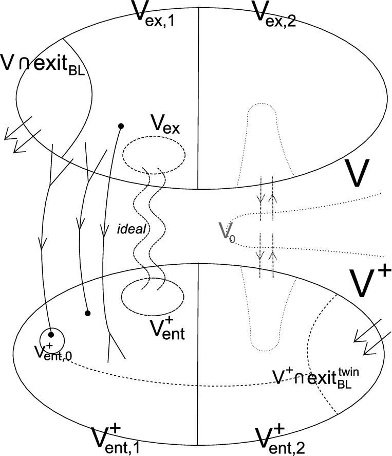
We define our partitions of the nearly $2$ -fair clusters as follows. For every $2$ -fair cluster $V$ with $V\cap{\rm exit}_{BL}\neq\emptyset$ we will choose a partition $V_{ex,1},V_{ex,2}$ of $V$ and a partition $V^{+}_{ent,1},V^{+}_{ent,2}$ of $V^{+}$ . Also, for every $2$ -fair cluster $V$ with $V\cap{\rm entry}_{BL}\neq\emptyset$ we choose a partition $V_{ent,1},V_{ent,2}$ of $V$ and a partition $V^{-}_{ex,1},V^{-}_{ex,2}$ of $V^{-}$ . There is no conflict in our notation, i.e. we will not e.g. define $V_{ex,1}$ twice, since when $V\cap{\rm exit}_{BL}\neq\emptyset$ we must have $V\in B$ , whereas when $V^{+}\cap{\rm entry}_{BL}\neq\emptyset$ we must have $V^{+}\in L$ , so $V\in T$ , and these cannot occur simultaneously. We also define the analogous partitions with respect to ${\rm Match}_{TR}$ , although for simplicity we will not explicitly introduce notation for them, as we will mainly focus on the case when only ${\rm Match}_{BL}$ is needed for the argument. So for each cluster $V$ we will choose at most $4$ partitions. We let $V_{{\rm 2nd}}$ be the intersection of all the second parts of the at most 4 partitions defined for $V$ . (So if all 4 partitions are defined, then $V_{\rm 2nd}$ is the intersection of the sets $V_{ex,2},V_{ent,2}$ defined with respect to ${\rm Match}_{BL}$ and the 2 analogous sets defined with respect to ${\rm Match}_{TR}$ . If only 3 partitions are defined for $V$ , then $V_{\rm 2nd}$ is the intersection of only 3 sets etc. If no partition is defined for $V$ , then $V_{\rm 2nd}=V$ .) We let $X_{\rm 2nd}$ be the union of $V_{\rm 2nd}$ over all clusters $V$ . We choose these partitions to satisfy the following lemma.

Lemma 31.

The partitions $V_{ex,1},V_{ex,2}$ and $V_{ent,1},V_{ent,2}$ can be chosen with the following properties (when they are defined).

(i)

$|V_{ex,1}|=m/2$ , $|V_{ent,1}|=m/2$ .
(ii)
For any $2$ -fair cluster $V$ with $V\cap{\rm exit}_{BL}\neq\emptyset$ we have $V_{ex,2}\cap{\rm exit}_{BL}=\emptyset$ . Moreover, there is a set $V^{+}_{ent,0}\subseteq V^{+}_{ent,1}$ of size at most $10\varepsilon m$ such that:
- $\bullet$
  
  Each vertex in $V^{+}\setminus V^{+}_{ent,0}$ has at least $dm/40$ inneighbours in $V_{ex,1}\setminus{\rm exit}_{BL}$ .
- $\bullet$
  
  Each vertex in $V^{+}_{ent,0}$ has at least $dm/8$ inneighbours in $V_{ex,1}$ .
- $\bullet$
  
  Each vertex in $V$ has at least $dm/20$ outneighbours in $V^{+}_{ent,1}$ .
(iii)
For any $2$ -fair cluster $V$ with $V\cap{\rm entry}_{BL}\neq\emptyset$ we have $V_{ent,2}\cap{\rm entry}_{BL}=\emptyset$ . Moreover, there is a set $V^{-}_{ex,0}\subseteq V^{-}_{ex,1}$ of size at most $10\varepsilon m$ such that:
- $\bullet$
  
  Each vertex in $V^{-}\setminus V^{-}_{ex,0}$ has at least $dm/40$ outneighbours in $V_{ent,1}\setminus{\rm entry}_{BL}$ .
- $\bullet$
  
  Each vertex in $V^{-}_{ex,0}$ has at least $dm/8$ outneighbours in $V_{ent,1}$ .
- $\bullet$
  
  Each vertex in $V$ has at least $dm/20$ inneighbours in $V^{-}_{ex,1}$ .

Also, the analogues of statements (i)–(iii) for ${\rm Match}_{TR}$ hold. Moreover,

(iv)

Every vertex in $V_{0}$ has at least $\beta n/20$ inneighbours and at least $\beta n/20$ outneighbours in $X_{\rm 2nd}$ .
(v)

If $d^{+}_{(1-\beta)n/2}(G)\geqslant n/2$ then there are sets $S^{\prime}_{B}\subseteq\widetilde{B}\cap X_{\rm 2nd}$ and $S^{\prime}_{T}\subseteq\widetilde{T}\cap X_{\rm 2nd}$ such that $|S^{\prime}_{B}|,|S^{\prime}_{T}|\geqslant\beta n/80$ and such that every vertex in $S^{\prime}_{B}\cup S^{\prime}_{T}$ has outdegree at least $n/2$ in $G$ .
(vi)

If $d^{-}_{(1-\beta)n/2}(G)\geqslant n/2$ then there are sets $S^{\prime}_{L}\subseteq\widetilde{L}\cap X_{\rm 2nd}$ and $S^{\prime}_{R}\subseteq\widetilde{R}\cap X_{\rm 2nd}$ such that $|S^{\prime}_{L}|,|S^{\prime}_{R}|\geqslant\beta n/80$ and such that every vertex in $S^{\prime}_{L}\cup S^{\prime}_{R}$ has indegree at least $n/2$ in $G$ .

Proof.

Consider a $2$ -fair cluster $V$ with $V\cap{\rm exit}_{BL}\neq\emptyset$ . If $|V\cap{\rm exit}_{BL}|<20\varepsilon m$ we set $V^{+}_{ent,0}=\emptyset$ . Otherwise, if $|V\cap{\rm exit}_{BL}|\geqslant 20\varepsilon m$ we define $V^{+}_{ent,0}$ to be the set of vertices in $V^{+}$ that have less than $\frac{d}{8}|V\setminus{\rm exit}_{BL}|$ inneighbours in $V\setminus{\rm exit}_{BL}$ . Recall that $(V,V^{+})_{G^{\prime}}$ is $(10\varepsilon,d/4)$ -super-regular. Since $V$ is $2$ -fair we deduce that $|V^{+}_{ent,0}|\leqslant 10\varepsilon m$ .

Now consider constructing a partition of $V$ into $V_{ex,1}$ and $V_{ex,2}$ as follows. Include $V\cap{\rm exit}_{BL}$ into $V_{ex,1}$ and distribute the remaining vertices of $V$ between $V_{ex,1}$ and $V_{ex,2}$ so that $|V_{ex,1}|=m/2$ (recall that $m$ is even), choosing uniformly at random between all possibilities. Note that since $V$ is $2$ -fair the probability that a vertex of $V\setminus{\rm exit}_{BL}$ is included in $V_{ex,1}$ is at least $1/3$ . Then by the Chernoff bound for the hypergeometric distribution (Proposition 9), with high probability each vertex in $V^{+}\setminus V^{+}_{ent,0}$ has at least $\frac{1}{4}\frac{d}{8}|V\setminus{\rm exit}_{BL}|\geqslant dm/40$ inneighbours in $V_{ex,1}\setminus{\rm exit}_{BL}$ . Also, by definition of $V_{ent,0}^{+}$ and super-regularity, each vertex in $V^{+}_{ent,0}$ has at least $dm/4-\frac{d}{8}|V\setminus{\rm exit}_{BL}|\geqslant dm/8$ inneighbours in $V_{ex,1}$ . Next, consider similarly constructing a partition of $V^{+}$ into $V_{ent,1}^{+}$ and $V_{ent,2}^{+}$ as follows. Include $V_{ent,0}^{+}$ into $V_{ent,1}^{+}$ and distribute the remaining vertices of $V^{+}$ uniformly at random between $V_{ent,1}^{+}$ and $V_{ent,2}^{+}$ so that $|V_{ent,1}^{+}|=m/2$ . Note that any vertex in $V$ has outdegree at least $dm/4-|V^{+}_{ent,0}|\geqslant dm/5$ in $V^{+}\setminus V^{+}_{ent,0}$ . Again, the probability that a given vertex from $V^{+}\setminus V^{+}_{ent,0}$ is included in $V_{ent,1}^{+}$ is at least $1/3$ , so with high probability each vertex in $V$ has at least $(dm/5)/4=dm/20$ outneighbours in $V^{+}_{ent,1}$ . This shows the existence of the partitions required for (ii). The existence of partitions satisfying (iii) is proven in the same way.

For each vertex $v$ in a cluster $V$ which does not lie in ${\rm exit}_{BL}\cup V_{ent,0}\cup{\rm entry}_{BL}\cup V_{ex,0}$ or the analogous set defined with respect to ${\rm Match}_{TR}$ , the probability that it lies in the second part of each of the (up to) 4 partitions defined on $V$ (and thus lies in $X_{\rm 2nd}$ ) is at least $(1/2)^{4}$ . Since $\delta^{0}(G)\geqslant\beta n$ , a Chernoff bound (Proposition 9) implies that we can also choose the partitions to satisfy (iv).

Now suppose that $d^{+}_{(1-\beta)n/2}(G)\geqslant n/2$ . Then $G$ contains at least $(1+\beta)n/2$ vertices of outdegree at least $n/2$ . So Lemma 27(ii) implies that $\widetilde{B}$ contains a set $\widetilde{B}^{\prime}_{\rm large}$ of at least $\beta n/3$ vertices whose outdegree in $G$ is at least $n/2$ . $\widetilde{B}^{\prime}_{\rm large}$ in turn contains a set $\widetilde{B}_{\rm large}$ of at least $\beta n/4$ vertices which do not lie in ${\rm exit}_{BL}\cup V_{ent,0}\cup{\rm entry}_{BL}\cup V_{ex,0}$ (for any cluster $V$ ) or in the analogous set defined with respect to ${\rm Match}_{TR}$ . Similarly as for (iv), with high probability we have $|\widetilde{B}_{\rm large}\cap X_{\rm 2nd}|\geqslant(\beta n/4)/20$ . Similar arguments applied to $\widetilde{T}$ , $\widetilde{L}$ and $\widetilde{R}$ show that we can choose the partitions to satisfy (v) and (vi). ∎

8.4. The exceptional set

Next we will assign each vertex $x$ in the exceptional set $V_{0}$ an in-type which is one of $T$ or $B$ and an out-type which is one of $L$ or $R$ . Combining these two types together we will say each vertex of $V_{0}$ gets a type of the form $TR,TL,BR$ or $BL$ . We will also abuse notion and think of $TL$ as the set of all vertices of $V_{0}$ of in-type $T$ and out-type $L$ , etc. We write $\widetilde{T}^{*}$ for the set of all those vertices which belong to the set $X_{\rm 2nd}$ defined in the previous subsection as well as to clusters of $T$ which are $5$ -excellent with respect to both ${\rm Match}_{BL}$ and ${\rm Match}_{TR}$ . The other sets $\widetilde{B}^{*}$ etc. are defined similarly.

Lemma 32.

We can assign each vertex $x\in V_{0}$ an in- and an out-type such that the following conditions are satisfied.

(i)

There is a matching ${\rm Match}_{T}$ from $\widetilde{T}^{*}$ to the set of vertices of in-type $T$ .
(ii)

There is a matching ${\rm Match}_{B}$ from $\widetilde{B}^{*}$ to the set of vertices of in-type $B$ .
(iii)

There is a matching ${\rm Match}_{L}$ from the set of vertices of out-type $L$ to $\widetilde{L}^{*}$ .
(iv)

There is a matching ${\rm Match}_{R}$ from the set of vertices of out-type $R$ to $\widetilde{R}^{*}$ .
(v)

The endvertices of the matchings ${\rm Match}_{T}$ , ${\rm Match}_{B}$ , ${\rm Match}_{L}$ , ${\rm Match}_{R}$ in $V(G)\setminus V_{0}$ are all distinct. Let $V^{*}_{0}$ denote the set of all these endvertices.
(vi)

No cluster of $R_{G^{\prime}}$ contains more than $\gamma m$ vertices of $V_{0}^{*}$ .
(vii)

Subject to the above conditions, $\lvert|TR|-|BL|\rvert$ is minimal.

Proof.

To show that such a choice is possible, we claim that we can proceed sequentially through the vertices of $V_{0}$ , assigning in-types and out-types and greedily extending the appropriate matchings. Since $|V_{0}|\leqslant d^{1/4}n$ by (3), at any stage in this process we have constructed at most $2d^{1/4}n$ edges of the matchings ${\rm Match}_{T}$ , ${\rm Match}_{B}$ , ${\rm Match}_{L}$ , ${\rm Match}_{R}$ , and so there are at most $2d^{1/4}n/\gamma\leqslant d^{1/5}n$ vertices belonging to clusters which contain at least $\gamma m$ endpoints of the matchings. In addition, we have to avoid all the at most $800\eta n$ vertices lying in clusters which are not $5$ -excellent with respect to both ${\rm Match}_{BL}$ and ${\rm Match}_{TR}$ . So in total we have to avoid at most $801\eta n$ vertices in each step. But by Lemma 31(iv) each exceptional vertex has in- and outdegree at least $\beta n/20$ in $X_{\rm 2nd}$ , so Lemma 27(ii) implies that any vertex has at least $\beta n/50$ inneighbours in $\widetilde{T}\cap X_{\rm 2nd}$ or at least $\beta n/50$ inneighbours in $\widetilde{B}\cap X_{\rm 2nd}$ . A similar statement holds for outneighbours in $\widetilde{L}\cap X_{\rm 2nd}$ or $\widetilde{R}\cap X_{\rm 2nd}$ , Thus a greedy procedure can satisfy conditions (i)–(vi), and then we can choose an assignment to satisfy (vii). ∎

Note that one advantage of choosing $V_{0}^{*}$ in $X_{\rm 2nd}$ is that $V_{0}^{*}$ will be disjoint from the sets ${\rm Entry}_{BL}$ etc. The strategy of the remaining proof depends on the value of $|TR|-|BL|$ . We will only consider the case $|TR|-|BL|\geqslant 0$ , as the argument for $|TR|-|BL|\leqslant 0$ is identical, under the symmetry $L\leftrightarrow R$ , $T\leftrightarrow B$ . When $|TR|>|BL|$ only ${\rm Match}_{BL}$ is needed for the argument. When $|TR|=|BL|$ we do not need either pseudo-matching, although the case $|TR|=|BL|=0$ has additional complications.

8.5. Twins

When $|TR|>|BL|$ , we obtain one type of transitions from $\widetilde{B}$ to $\widetilde{L}$ by fixing a pseudo-matching ${\rm Match}^{\prime}_{BL}\subseteq{\rm Match}_{BL}$ . The other type of transitions uses a set ${\rm Entry}_{RL}\subseteq\widetilde{M}_{V}^{RL}$ , as explained below. We define exits ${\rm Exit}_{BL}\subseteq{\rm exit}_{BL}$ and entries ${\rm Entry}_{BL}\subseteq{\rm entry}_{BL}$ of ${\rm Match}^{\prime}_{BL}$ as for ${\rm Match}_{BL}$ . Lemma 34(i) below implies that $|{\rm Match}_{BL}|+|\widetilde{M}_{V}^{RL}|\geqslant|TR|-|BL|.$ Thus we can fix sets ${\rm Match}^{\prime}_{BL}$ and ${\rm Entry}_{RL}$ to satisfy

|{\rm Match}^{\prime}_{BL}|+|{\rm Entry}_{RL}|=|TR|-|BL|.

For each edge $xy\in{\rm Match}^{\prime}_{BL}$ we will choose ‘twins’ $x^{twin}$ and $y^{twin}$ of its endpoints. To use the edge $xy$ in our shifted walk $W$ , we will enter the cycle of $F$ containing $x$ at $x^{twin}$ , wind around the cycle to $x$ , use the edge $xy$ , wind around the cycle containing $y$ , and then leave it at $y^{twin}$ . A vertex that is the midpoint of a directed path of length 2 in ${\rm Match}^{\prime}_{BL}$ will actually have two twins, but we will not complicate the notation to reflect this, as it will be clear from the context which twin is intended. Thus we obtain two ‘twin maps’ $x\mapsto x^{twin}$ and $y\mapsto y^{twin}$ . We also use the notation $S^{twin}=\{x^{twin}:x\in S\}$ when $S$ is a set of vertices. The twin maps will be injective on ${\rm Exit}_{BL}$ and on ${\rm Entry}_{BL}$ , in that $|{\rm Exit}_{BL}|=|{\rm Exit}_{BL}^{twin}|$ , $|{\rm Entry}_{BL}|=|{\rm Entry}_{BL}^{twin}|$ , and moreover $|V\cap{\rm Exit}_{BL}|=|V^{+}\cap{\rm Exit}_{BL}^{twin}|$ , $|V\cap{\rm Entry}_{BL}|=|V^{-}\cap{\rm Entry}_{BL}^{twin}|$ .

Our choice of $x^{twin}$ depends on whether the cluster $V$ containing $x$ is $2$ -fair with respect to ${\rm Match}_{BL}$ . If $V$ is not $2$ -fair then we fix arbitrary perfect matchings in $G^{\prime}$ from $V^{-}$ to $V$ and from $V$ to $V^{+}$ (using Lemma 12). Then for every $x\in V\cap{\rm Exit}_{BL}$ we let $x^{twin}$ be the vertex $x$ is matched to in $V^{+}$ and for every $x\in V\cap{\rm Entry}_{BL}$ we let $x^{twin}$ be the vertex in $V^{-}$ matched to $x$ .

On the other hand, if $V$ is $2$ -fair then we make use of the partitions defined in Lemma 31. If $V\cap{\rm Exit}_{BL}\neq\emptyset$ then we choose twins for vertices in $V\cap{\rm Exit}_{BL}$ within $(V^{+}_{ent,2}\cup V^{+}_{ent,0})\setminus V^{*}_{0}$ , arbitrarily subject to the condition that if $|V\cap{\rm Exit}_{BL}|>20\varepsilon m$ then $(V\cap{\rm Exit}_{BL})^{twin}$ contains $V^{+}_{ent,0}$ . (Recall that $V^{*}_{0}$ was defined in Lemma 32(v).) If $V$ is $2$ -fair, we will also choose some ideal of $(V\setminus{\rm Exit}_{BL},V^{+}\setminus{\rm Exit}_{BL}^{twin})_{G^{\prime}}$ to create flexibility when selecting further sets while preserving super-regularity. To do this, recall that $(V,V^{+})_{G^{\prime}}$ was $(10\varepsilon,d/4)$ -super-regular. Together with Lemma 31(i),(ii) this implies that $(V_{ex,1}\setminus{\rm Exit}_{BL},V^{+}_{ent,1}\setminus{\rm Exit}_{BL}^{twin})_{G^{\prime}}$ is $(30\varepsilon,d/40)$ -super-regular. Next we randomly choose sets $V_{ex}\subseteq V_{ex,1}\setminus{\rm Exit}_{BL}$ and $V^{+}_{ent}\subseteq V^{+}_{ent,1}\setminus{\rm Exit}_{BL}^{twin}$ of size $80dm$ . Lemma 15 (applied with $\theta=160d$ and $n=m/2$ ) implies that with high probability $(V_{ex},V^{+}_{ent})$ is an $(\sqrt{\varepsilon},d^{2})$ -ideal for $(V_{ex,1}\setminus{\rm Exit}_{BL},V^{+}_{ent,1}\setminus{\rm Exit}_{BL}^{twin})_{G^{\prime}}$ . Moreover, Lemma 31(ii) and the Chernoff bound (Proposition 9) together imply that with high probability every vertex in $V_{ex,2}$ has at least $d^{2}m$ outneighbours in $V^{+}_{ent}$ while every vertex in $V^{+}_{ent,2}$ has at least $d^{2}m$ inneighbours in $V_{ex}$ . Altogether this shows that we can choose $(V_{ex},V^{+}_{ent})$ to be a $(\sqrt{\varepsilon},d^{2})$ -ideal for $(V\setminus{\rm Exit}_{BL},V^{+}\setminus{\rm Exit}_{BL}^{twin})_{G^{\prime}}$ .

Similarly, if $V\cap{\rm Entry}_{BL}\neq\emptyset$ then we choose twins for vertices in $V\cap{\rm Entry}_{BL}$ in $(V^{-}_{ex,2}\cup V^{-}_{ex,0})\setminus V_{0}^{*}$ , arbitrarily subject to the condition that if $|V\cap{\rm Entry}_{BL}|>20\varepsilon m$ then $(V\cap{\rm Entry}_{BL})^{twin}$ contains $V^{-}_{ex,0}$ . We also choose a $(\sqrt{\varepsilon},d^{2})$ -ideal $(V^{-}_{ex},V_{ent})$ for $(V^{-}\setminus{\rm Entry}_{BL}^{twin},V\setminus{\rm Entry}_{BL})_{G^{\prime}}$ . Then we define $X_{BL}$ to be the union of the sets $V_{ex}$ and $V_{ent}$ defined using ${\rm Match}^{\prime}_{BL}$ over all nearly 2-fair clusters $V$ . Note that these sets will play a similar role to the sets $V^{*}$ used in the highly connected case, in that they preserve super-regularity even if when some vertices are deleted. We let

X^{*}_{BL}:=X_{BL}\cup{\rm Exit}_{BL}\cup{\rm Entry}_{BL}\cup{\rm Exit}^{twin}_{BL}\cup{\rm Entry}^{twin}_{BL}.

Note that $X^{*}_{BL}\cap V^{*}_{0}=\emptyset$ . Define $X_{TR}$ and $X^{*}_{TR}$ similarly using the matching ${\rm Match}^{\prime}_{TR}$ .

We will also choose twins for vertices in ${\rm Entry}_{RL}$ such that if $x\in V\in M_{V}^{RL}$ then $x^{twin}\in V^{-}\in M_{H}^{RL}$ . Lemma 29(iii),(iv) implies that each $x\in{\rm Entry}_{RL}$ has many inneighbours in $\widetilde{B}$ while $x^{twin}$ has many outneighbours in $\widetilde{L}$ . Writing $C$ for the cycle of $F$ containing the cluster containing $x$ , we get a transition from $\widetilde{B}$ to $\widetilde{L}$ by entering $C$ at $x$ from an inneighbour in $\widetilde{B}$ , traversing $C$ , then exiting $C$ at $x^{twin}$ to an outneighbour in $\widetilde{L}$ .

Now we describe how to choose twins for ${\rm Entry}_{RL}$ , and also some ideals to create flexibility while preserving super-regularity. Call a cluster $V$ $M^{RL}$ -full if it contains at least $\gamma m$ vertices in ${\rm Entry}_{RL}$ . Say $V$ is $\ell$ -good (with respect to ${\rm Match}_{BL}$ and ${\rm Entry}_{RL}$ ) if $V$ is $\ell$ -fair with respect to ${\rm Match}_{BL}$ and no cluster with distance at most $\ell$ from $V$ on $F$ is $M^{RL}$ -full. Since $|{\rm Entry}_{RL}|\leqslant|V_{0}|\leqslant d^{1/4}n$ the number of $M^{RL}$ -full clusters is at most $\gamma^{-1}d^{1/4}n/m$ . Recalling that by ( $\clubsuit$ ) at most $3\gamma k$ clusters are full,

at most

9(3\gamma k+\gamma^{-1}d^{1/4}n/m)\leqslant 30\gamma k

clusters are not

4

-good.

(♢)

Consider a cluster $V\in M_{V}^{RL}$ with $V\cap{\rm Entry}_{RL}\neq\emptyset$ . If $V$ is not $2$ -good then we choose a perfect matching in $G^{\prime}$ from $V^{-}$ to $V$ (using Lemma 12), and for each $x\in V$ let $x^{twin}$ be the vertex in $V^{-}$ that is matched to $x$ . Now suppose that $V$ is $2$ -good. Then none of $V^{-}$ , $V$ and $V^{+}$ is full with respect to ${\rm Match}_{BL}$ or $M^{RL}$ -full. Since $(V^{-},V)_{G^{\prime}}$ is $(10\varepsilon,d/4)$ -super-regular and $|V\cap{\rm Entry}_{RL}|<\gamma m$ we can apply Lemma 14 to obtain a set $Y\subseteq V^{-}$ with $|Y|=|V\cap{\rm Entry}_{RL}|$ such that $(V^{-}\setminus Y,V\setminus{\rm Entry}_{RL})_{G^{\prime}}$ is $(20\varepsilon,d/8)$ -super-regular. Then we let the twin map be an arbitrary bijection from $V\cap{\rm Entry}_{RL}$ to $Y$ . Next we apply Lemma 15 with $\theta=32d$ to obtain a $(\sqrt{\varepsilon},d^{2})$ -ideal for $(V^{-}\setminus{\rm Entry}_{RL}^{twin},V\setminus{\rm Entry}_{RL})_{G^{\prime}}$ , which we will call $(V^{-}_{ex},V_{ent})$ . (Similarly to the earlier argument and the one in the next paragraph, the partitions of $V(G)\setminus V_{0}$ into $\widetilde{L}$ , $\widetilde{R}$ and $\widetilde{M}_{V}$ and into $\widetilde{T}$ , $\widetilde{B}$ and $\widetilde{M}_{H}$ guarantee that there is no conflict with our previous notation.) Now we define

X^{*}_{RL}:=\bigcup_{V\in M_{V}^{RL}}V_{ent}\cup\bigcup_{V\in M_{H}^{RL}}V_{ex}\cup{\rm Entry}_{RL}\cup{\rm Entry}_{RL}^{twin},

X^{*}:=X^{*}_{BL}\cup X^{*}_{RL}.

(4)

Then $|X^{*}|\leqslant\gamma n$ and $X^{*}\cap V^{*}_{0}=\emptyset$ . (The latter follows since the vertices in $V^{*}_{0}$ lie in 5-excellent clusters and so $X^{*}_{RL}\cap V^{*}_{0}=\emptyset$ .) We also define

V_{entry}:=V\cap({\rm Entry}_{BL}\cup{\rm Exit}_{BL}^{twin}\cup{\rm Entry}_{RL}),

V_{exit}:=V\cap({\rm Exit}_{BL}\cup{\rm Entry}_{BL}^{twin}\cup{\rm Entry}_{RL}^{twin}).

Note that ${\rm Entry}_{BL}\subseteq\widetilde{L}$ , ${\rm Exit}_{BL}^{twin}\subseteq\widetilde{R}$ and ${\rm Entry}_{RL}\subseteq\widetilde{M}_{V}^{RL}$ . Since $\widetilde{L}$ , $\widetilde{R}$ and $\widetilde{M}_{V}$ partition $V(G)\setminus V_{0}$ , any vertex will be used at most once to enter a cluster. In particular,

V_{entry}=\begin{cases}V\cap{\rm Entry}_{BL}&\text{if }V\in L;\\ V\cap{\rm Exit}_{BL}^{twin}&\text{if }V\in R;\\ V\cap{\rm Entry}_{RL}&\text{if }V\in M_{V}^{RL}.\end{cases}

Similarly, ${\rm Exit}_{BL}\subseteq\widetilde{B}$ , ${\rm Entry}_{BL}^{twin}\subseteq\widetilde{T}$ and ${\rm Entry}_{RL}^{twin}\subseteq\widetilde{M}_{H}^{RL}$ . Since $\widetilde{T}$ , $\widetilde{B}$ and $\widetilde{M}_{H}$ also partition $V(G)\setminus V_{0}$ , any vertex will be used at most once to exit a cluster and

V_{exit}=\begin{cases}V\cap{\rm Exit}_{BL}&\text{if }V\in B;\\ V\cap{\rm Entry}_{BL}^{twin}&\text{if }V\in T;\\ V\cap{\rm Entry}_{RL}^{twin}&\text{if }V\in M_{H}^{RL}.\end{cases}

Some vertices may be used for both exits and entrances, and they will have two twins. We summarise the properties of twins with the following lemma.

Lemma 33.

Suppose that $|TR|>|BL|$ . Then

(i)

$|{\rm Match}^{\prime}_{BL}|+|{\rm Entry}_{RL}|=|TR|-|BL|$ .
(ii)

Every cluster intersects at most one of ${\rm Entry}_{BL}$ , ${\rm Exit}_{BL}^{twin}$ , ${\rm Entry}_{RL}$ . Similarly, every cluster intersects at most one of ${\rm Exit}_{BL}$ , ${\rm Entry}_{BL}^{twin}$ , ${\rm Entry}_{RL}^{twin}$ .
(iii)

There exists a perfect matching from $V\setminus V_{exit}$ to $V^{+}\setminus V^{+}_{entry}$ .
(iv)
Suppose $V$ is $3$ -good with respect to ${\rm Match}_{BL}$ and ${\rm Entry}_{RL}$ . Then
- $\bullet$
  
  For all sets $X^{\prime}$ and $Y^{\prime}$ with $(V\cap X^{*})\setminus V_{exit}\subseteq X^{\prime}\subseteq V\setminus V_{exit}$ and $(V^{+}\cap X^{*})\setminus V^{+}_{entry}\subseteq Y^{\prime}\subseteq V^{+}\setminus V^{+}_{entry}$ the pair $(X^{\prime},Y^{\prime})_{G^{\prime}}$ is $(\sqrt{\varepsilon},d^{2})$ -super-regular.
- $\bullet$
  
  For all sets $X^{\prime}$ and $Y^{\prime}$ with $(V\cap X^{*})\setminus V_{entry}\subseteq X^{\prime}\subseteq V\setminus V_{entry}$ and $(V^{-}\cap X^{*})\setminus V^{-}_{exit}\subseteq Y^{\prime}\subseteq V^{-}\setminus V^{-}_{exit}$ the pair $(Y^{\prime},X^{\prime})_{G^{\prime}}$ is $(\sqrt{\varepsilon},d^{2})$ -super-regular.

Proof.

As discussed at the beginning of the subsection, Lemma 34(i) will allow us to choose ${\rm Match}^{\prime}_{BL}$ and ${\rm Entry}_{RL}$ of the size required in (i). Property (ii) was discussed above. We will just consider the first point of property (iv), as the second is similar. Suppose $V$ is $3$ -good and consider sets $X^{\prime}$ and $Y^{\prime}$ as in the statement. We need to show that $(X^{\prime},Y^{\prime})_{G^{\prime}}$ is $(\sqrt{\varepsilon},d^{2})$ -super-regular. If $V\cap{\rm Entry}_{RL}^{twin}\neq\emptyset$ this holds by definition of $X^{*}_{RL}$ since $V_{ex}\cap V_{exit}=\emptyset$ and $V_{ent}^{+}\cap V_{entry}^{+}=\emptyset$ by (ii) (and so $V_{ex}\subseteq X^{\prime}$ and $V^{+}_{ent}\subseteq Y^{\prime}$ ), and since $V^{+}$ is $2$ -good. If $V\cap{\rm Exit}_{BL}\neq\emptyset$ this holds by definition of $X^{*}_{BL}$ , since $V$ is $2$ -fair, and similarly, if $V\cap{\rm Entry}_{BL}^{twin}\neq\emptyset$ this holds again by definition of $X^{*}_{BL}$ , since $V^{+}$ is $2$ -fair. It remains to prove property (iii). Suppose first that $V\in M_{H}^{RL}$ . If $V^{+}$ is not $2$ -good then the required matching exists by the way we defined twins for ${\rm Entry}_{RL}$ in this case. On the other hand, if $V^{+}$ is $2$ -good then we can apply the super-regularity property (iv) just established (which only used the fact that $V^{+}$ is $2$ -good) and Lemma 12. Next suppose that $V\in B$ . Then $V_{exit}=V\cap{\rm Exit}_{BL}$ and $V^{+}_{entry}=V^{+}\cap{\rm Exit}_{BL}^{twin}$ . Thus if $V$ is not $2$ -fair then the required matching exists by the way we defined twins for ${\rm Match}^{\prime}_{BL}$ in this case. On the other hand, if $V$ is $2$ -fair then we can apply the first point of property (iv), which only used the fact that $V$ is $2$ -fair. Similarly, when $V\in T$ , then $V_{exit}=V\cap{\rm Entry}_{BL}^{twin}$ and $V^{+}_{entry}=V^{+}\cap{\rm Entry}_{BL}$ . If $V^{+}$ is not $2$ -fair the required matching exists by the construction in this case, whereas if $V^{+}$ is $2$ -fair then we can apply the second point of property (iv) with $(V,V^{+})$ playing the role of $(V^{-},V)$ , which only uses the fact that $V^{+}$ (playing the role of $V$ in the second point) is $2$ -fair. ∎

8.6. Summary

The auxiliary graph $H$ is decomposed into shifted components $L$ ‘left’ and $R$ ‘right’ of size $k/2\pm 19\eta k$ and a set $M_{V}$ of size $|M_{V}|<17\eta k$ . This corresponds to a partition of $V(G)\setminus V_{0}=\widetilde{L}\cup\widetilde{R}\cup\widetilde{M}_{V}$ . The $1$ -factor $F$ defines a partition $V(H)=T\cup B\cup M_{H}$ , where a cluster $V$ belongs to $T,B,M_{H}$ if and only if its successor $V^{+}$ belongs to $L,R,M_{V}$ respectively. The shifted walk $W$ will use two types of transitions from $\widetilde{B}$ to $\widetilde{L}$ . One type is a pseudo-matching ${\rm Match}^{\prime}_{BL}$ from $\widetilde{B}$ to $\widetilde{L}$ , matching ${\rm Exit}_{BL}$ to ${\rm Entry}_{BL}$ . The other type is a set ${\rm Entry}_{RL}$ of vertices in $\widetilde{M}_{V}^{RL}\subseteq\widetilde{M}_{V}$ , with the property that if $V\in M_{V}^{RL}$ then any $x\in V$ has many inneighbours in $\widetilde{B}$ and any $y\in V^{-}$ has many outneighbours in $\widetilde{L}$ . We did not discuss transitions from $\widetilde{T}$ to $\widetilde{R}$ , but these are obtained similarly under the transformation $L\leftrightarrow R$ , $B\leftrightarrow T$ , etc. Each vertex in these sets has a twin (or possibly two twins) that will be used when $W$ traverses the cycle of $F$ containing it. For any cluster $V$ , the set of exit points from $V$ is $V_{exit}$ and the set of entry points to $V$ is $V_{entry}$ . There exists a perfect matching from $V\setminus V_{exit}$ to $V^{+}\setminus V^{+}_{entry}$ . The exceptional set $V_{0}$ is decomposed into $4$ parts $TR$ , $TL$ , $BR$ and $BL$ , where the first letter gives the in-type of a vertex and the second letter the out-type: there is a matching ${\rm Match}_{T}$ from $\widetilde{T}^{*}$ to vertices of in-type $T$ (and so on). Technical complications are created by the possibility that a cluster may be full (contain at least $\gamma m$ endpoints of ${\rm Match}_{BL}$ ) or $M^{RL}$ -full (contain at least $\gamma m$ endpoints of ${\rm Entry}_{RL}$ ). A cluster $V$ is $\ell$ -fair if no cluster at distance at most $\ell$ from $V$ is full, $\ell$ -excellent if no cluster at distance at most $\ell$ from $V$ is full or in $M=M_{V}\cup M_{H}$ , and $\ell$ -good if no cluster at distance at most $\ell$ from $V$ is full or $M^{RL}$ -full. We have a set $X^{*}=X^{*}_{BL}\cup X^{*}_{RL}$ such that whenever $V$ is $3$ -good, we have flexibility to use any vertices avoiding these sets in $V^{-}$ , $V$ and $V^{+}$ (as well as avoiding the exits and entries already chosen), while preserving super-regularity of the corresponding pairs in $F$ . Finally, the set $V^{*}_{0}$ of endpoints in $V(G)\setminus V_{0}$ of the matchings ${\rm Match}_{T}$ etc. only uses $5$ -excellent clusters and avoids $X^{*}$ .

9. The size of the pseudo-matching

Our aim in this section is to prove the following lower bound on the size of our pseudo-matchings ${\rm Match}_{BL}$ and ${\rm Match}_{TR}$ .

Lemma 34.

(i)

$|{\rm Match}_{BL}|\geqslant\min\{|\widetilde{M}_{V}^{LR}|/2,\gamma^{4}n\}-|\widetilde{M}_{V}^{RL}|-|V_{0}|$ . Moreover, if $|TR|>|BL|$ then $|{\rm Match}_{BL}|\geqslant|TR|-|BL|-|\widetilde{M}_{V}^{RL}|+\min\{|\widetilde{M}_{V}^{LR}|/2,\gamma^{4}n\}$ .
(ii)

$|{\rm Match}_{TR}|\geqslant\min\{|\widetilde{M}_{V}^{RL}|/2,\gamma^{4}n\}-|\widetilde{M}_{V}^{LR}|-|V_{0}|$ . Moreover, if $|BL|>|TR|$ then $|{\rm Match}_{TR}|\geqslant|BL|-|TR|-|\widetilde{M}_{V}^{LR}|+\min\{|\widetilde{M}_{V}^{RL}|/2,\gamma^{4}n\}$ .

To prove this we first show that there are large sets $S_{B}\subseteq\widetilde{B}$ with many outneighbours in $\widetilde{L}$ and $S_{L}\subseteq\widetilde{L}$ with many inneighbours in $\widetilde{B}$ . Note that part (v) in the following lemma is not used in the proof of Lemma 34 but will be needed in the final section of the paper.

Lemma 35.

(i)

If $|TR|>|BL|$ there is $S_{B}\subseteq\widetilde{B}$ with $|S_{B}|\geqslant\beta n/100$ , such that every $x\in S_{B}$ satisfies

|N^{+}_{G}(x)\cap\widetilde{L}|\geqslant\deg_{L}:=\frac{n}{2}-(|BL|+|BR|+|\widetilde{R}|)-|\widetilde{M}^{RL}_{V}|-|\widetilde{M}^{LR}_{V}|/4.

Furthermore, in any case, $\widetilde{B}$ contains a set $S^{*}_{B}$ of size $|S^{*}_{B}|\geqslant\beta n/100$ , such that every $x\in S^{*}_{B}$ satisfies $|N^{+}_{G}(x)\cap\widetilde{L}|\geqslant\frac{n}{2}-|V_{0}|-|\widetilde{R}|-|\widetilde{M}^{RL}_{V}|-|\widetilde{M}^{LR}_{V}|/4$ .

(ii)

If $|TR|>|BL|$ there is $S_{L}\subseteq\widetilde{L}$ with $|S_{L}|\geqslant\beta n/100$ , such that every $x\in S_{L}$ satisfies

|N^{-}_{G}(x)\cap\widetilde{B}|\geqslant\deg_{B}:=\frac{n}{2}-(|TL|+|BL|+|\widetilde{T}|)-|\widetilde{M}^{RL}_{H}|-|\widetilde{M}^{LR}_{H}|/4.

Furthermore, in any case, $\widetilde{L}$ contains a set $S^{*}_{L}$ of size $|S^{*}_{L}|\geqslant\beta n/100$ , such that every $x\in S^{*}_{L}$ satisfies $|N^{-}_{G}(x)\cap\widetilde{B}|\geqslant\frac{n}{2}-|V_{0}|-|\widetilde{T}|-|\widetilde{M}^{RL}_{H}|-|\widetilde{M}^{LR}_{H}|/4$ .

(iii)

If $|BL|>|TR|$ there is $S_{T}\subseteq\widetilde{T}$ with $|S_{T}|\geqslant\beta n/100$ , such that every $x\in S_{T}$ satisfies

|N^{+}_{G}(x)\cap\widetilde{R}|\geqslant\deg_{R}:=\frac{n}{2}-(|TL|+|TR|+|\widetilde{L}|)-|\widetilde{M}^{LR}_{V}|-|\widetilde{M}^{RL}_{V}|/4.

Furthermore, in any case, $\widetilde{T}$ contains a set $S^{*}_{T}$ of size $|S^{*}_{T}|\geqslant\beta n/100$ , such that every $x\in S^{*}_{T}$ satisfies $|N^{+}_{G}(x)\cap\widetilde{R}|\geqslant\frac{n}{2}-|V_{0}|-|\widetilde{L}|-|\widetilde{M}^{LR}_{V}|-|\widetilde{M}^{RL}_{V}|/4$ .

(iv)

If $|BL|>|TR|$ there is $S_{R}\subseteq\widetilde{R}$ with $|S_{R}|\geqslant\beta n/100$ , such that every $x\in S_{R}$ satisfies

|N^{-}_{G}(x)\cap\widetilde{T}|\geqslant\deg_{T}:=\frac{n}{2}-(|TR|+|BR|+|\widetilde{B}|)-|\widetilde{M}^{LR}_{H}|-|\widetilde{M}^{RL}_{H}|/4.

Furthermore, in any case, $\widetilde{R}$ contains a set $S^{*}_{R}$ of size $|S^{*}_{R}|\geqslant\beta n/100$ , such that every $x\in S^{*}_{R}$ satisfies $|N^{-}_{G}(x)\cap\widetilde{T}|\geqslant\frac{n}{2}-|V_{0}|-|\widetilde{B}|-|\widetilde{M}^{LR}_{H}|-|\widetilde{M}^{RL}_{H}|/4$ .

(v)
Finally, suppose that $M_{V}^{RL}$ , $TR$ and $BL$ are all empty.
- $\bullet$
  
  If $|\widetilde{L}\cup TL|\geqslant|\widetilde{B}\cup BR|$ , then $\widetilde{B}$ contains a set $S_{B}$ of at least $\beta n/100$ vertices, each having at least $|\widetilde{M}_{V}^{LR}|/4$ outneighbours in $\widetilde{L}\cup TL$ .
- $\bullet$
  
  If $|\widetilde{L}\cup TL|\leqslant|\widetilde{B}\cup BR|$ , then $\widetilde{L}$ contains a set $S_{L}$ of at least $\beta n/100$ vertices, each having at least $|\widetilde{M}_{V}^{LR}|/4$ inneighbours in $\widetilde{B}\cup BR$ .

Proof.

Suppose that $|TR|>|BL|$ . To prove (i), we first consider the case when $d^{+}_{(1-\beta)n/2}(G)\geqslant n/2$ . Let $S^{\prime}_{B}$ be as defined in Lemma 31(v). Let $S_{B}$ be the set obtained from $S^{\prime}_{B}$ by deleting the following vertices.

•

The set $V_{0}^{*}$ of $2|V_{0}|\leqslant 2d^{1/4}n$ endvertices in $V(G)\setminus V_{0}$ of edges in ${\rm Match}_{T}$ , ${\rm Match}_{B}$ , ${\rm Match}_{L}$ , ${\rm Match}_{R}$ .
•

All the at most $800\eta n$ vertices which lie in clusters that are not $5$ -excellent with respect to ${\rm Match}_{BL}$ or ${\rm Match}_{TR}$ .
•

All the at most $2|V_{0}|k/(\gamma m/2)\leqslant d^{1/5}n$ vertices which lie in clusters containing at least $\gamma m/2$ vertices of $V_{0}^{*}$ .
•

All the at most $12\eta^{\prime}n$ vertices in $\widetilde{B}$ having more than $|\widetilde{M}^{LR}_{V}|/4$ outneighbours in $\widetilde{M}^{LR}_{V}$ (see Lemma 29(ii)).

Thus $|S_{B}|\geqslant\beta n/100$ . Now we make the following key use of the minimality of $|TR|-|BL|>0$ . We claim that any vertex $x\in S_{B}$ has outdegree at most $|BL|+|BR|$ in $V_{0}$ . Otherwise, there would be some edge $xy$ with $y\in TL\cup TR$ . But then we can change the in-type of $y$ to $B$ by deleting the edge in ${\rm Match}_{T}$ incident to $y$ and adding the edge $xy$ to ${\rm Match}_{B}$ . Conditions (v) and (vi) in Lemma 32 will still hold, since $S_{B}$ is disjoint from $V_{0}^{*}$ and only contains vertices in clusters containing at most $\gamma m/2$ vertices of $V_{0}^{*}$ . Condition (ii) holds since $x\in\widetilde{B}^{*}$ by definition of $S_{B}$ . This reduces $||TR|-|BL||$ , which contradicts the minimality condition in Lemma 32(vii). Therefore the claim holds. Now recall that $\widetilde{R}\cup\widetilde{L}\cup\widetilde{M}^{LR}_{V}\cup\widetilde{M}^{RL}_{V}\cup V_{0}$ is a partition of $V(G)$ . Any $x\in S_{B}$ has at least $n/2$ outneighbours, of which at most $|\widetilde{R}|+|\widetilde{M}^{RL}_{V}|$ belong to $\widetilde{R}\cup\widetilde{M}^{RL}_{V}$ , at most $|\widetilde{M}^{LR}_{V}|/4$ belong to $\widetilde{M}^{LR}_{V}$ and at most $|BL|+|BR|$ belong to $V_{0}$ . This shows that $S_{B}$ is a set as required in (i).

Now consider the case when $d^{+}_{(1-\beta)n/2}(G)<n/2$ , and so $d^{-}_{(1-\beta)n/2}(G)\geqslant(1+\beta)n/2$ by our degree assumptions. Then $G$ has at least $(1+\beta)n/2$ vertices of indegree at least $(1+\beta)n/2$ , and by Lemma 27 at least $(1+\beta)n/2-|\widetilde{R}|-|V_{0}|-|\widetilde{M}_{V}|>\beta n/3$ of these belong to $\widetilde{L}$ . Let $A\subseteq\widetilde{L}$ be a set of $\beta n/3$ vertices with indegree at least $(1+\beta)n/2$ . Note that every vertex in $A$ has indegree at least $(1+\beta)n/2+|\widetilde{B}|-n>\beta n/3$ in $\widetilde{B}$ . Then we must have a set $S_{B}$ of at least $\beta n/100$ vertices in $\widetilde{B}$ , each having outdegree at least $\beta^{3}n$ in $A$ , or we would have $\beta n/3\cdot|A|\leqslant E(\widetilde{B},A)\leqslant\beta n/100\cdot|A|+\beta^{3}n|\widetilde{B}|$ , a contradiction. Then every vertex in $S_{B}$ has at least $\beta^{3}n\geqslant\frac{n}{2}-|\widetilde{R}|$ outneighbours in $A\subseteq\widetilde{L}$ , as required. This completes the proof of (i) when $|TR|>|BL|$ .

The argument for (i) when we do not have $|TR|>|BL|$ is the same, except that we no longer have the minimality argument for $||TR|-|BL||$ , so vertices in $S^{*}_{B}$ may have all of $V_{0}$ as outneighbours. The arguments for (ii)–(iv) are analogous, so we omit them.

Finally, suppose that $M_{V}^{RL}$ , $TR$ and $BL$ are all empty, so that $\widetilde{R}\cup\widetilde{L}\cup\widetilde{M}^{LR}_{V}\cup TL\cup BR$ is a partition of $V(G)$ . For the first point in (v), suppose that $|\widetilde{L}\cup TL|\geqslant|\widetilde{B}\cup BR|$ . Since $|\widetilde{B}|=|\widetilde{R}|$ , every vertex $x$ in $S_{B}$ (defined as above) has at least $n/2-|BR|-|\widetilde{B}|-|\widetilde{M}_{V}^{LR}|/4$ outneighbours in $\widetilde{L}\cup TL$ . By assumption, we have $|BR|+|\widetilde{B}|+|\widetilde{M}_{V}^{LR}|/2\leqslant n/2$ , so the number of outneighbours of $x$ in $\widetilde{L}\cup TL$ is at least $|\widetilde{M}_{V}^{LR}|/4$ , as required. The second point follows in the same way.∎

Proof of Lemma 34. Observe that all stated lower bounds are at most $\gamma^{2}n$ , so it is enough to prove the existence of pseudo-matchings satisfying these bounds. We will suppose that $|TR|>|BL|$ and prove the ‘moreover’ statement of (i); the arguments for the other assertions are similar. Define an auxiliary bipartite graph whose vertex classes are $\widetilde{B}$ and $\widetilde{L}$ by joining a vertex $x\in\widetilde{B}$ to a vertex $y\in\widetilde{L}$ if $xy$ is an edge of $G$ . Let $J$ be the graph obtained from this bipartite graph by deleting all the edges whose endvertices both lie in clusters having distance at most 4 in $F$ from $M$ . Let $Q$ be the largest matching in $J$ .

Case 1. $|Q|\geqslant\gamma^{2}n$ .

Let $Q^{\prime}$ be a matching obtained from $Q$ by deleting as few edges as possible so as to ensure that every vertex of $G$ belongs to at most one edge from $Q^{\prime}$ . Note that every vertex of $G$ has indegree at most $1$ and outdegree at most $1$ in $Q$ , so $Q$ considered as a subdigraph of $G$ is a vertex-disjoint union of directed paths and cycles. Thus we can retain at least $1/3$ of the edges of $Q$ in $Q^{\prime}$ (with equality for a disjoint union of directed triangles). By deleting further edges if necessary we may assume that $|Q^{\prime}|=\gamma^{2}n/3$ .

We claim that there is a submatching $Q^{\prime\prime}$ of $Q^{\prime}$ of size at least $\gamma|Q^{\prime}|/3$ such that no cluster is full with respect to $Q^{\prime\prime}$ (i.e. every cluster contains at most $\gamma m$ endvertices of $Q^{\prime\prime}$ ). To see that such a $Q^{\prime\prime}$ exists, consider the submatching $Q^{\prime\prime}$ obtained from $Q^{\prime}$ by retaining every edge of $Q^{\prime}$ with probability $\gamma/2$ in $Q^{\prime\prime}$ , independently of all other edges of $Q^{\prime}$ . Then for any cluster $V$ , the expected number of endvertices of $Q^{\prime\prime}$ in $V$ is at most $\gamma m/2$ , and the expected size of $Q^{\prime\prime}$ is $\gamma|Q^{\prime}|/2$ . By Chernoff bounds we see that with high probability $Q^{\prime\prime}$ has the claimed properties.

Note that $Q^{\prime\prime}$ is a pseudo-matching from $\widetilde{B}$ to $\widetilde{L}$ , as by construction it is a matching, and by definition of $J$ every edge in $Q^{\prime\prime}$ has an endvertex in a $4$ -excellent cluster. Also, since $|V_{0}|\leqslant d^{1/4}n$ we have $|Q^{\prime\prime}|\geqslant\gamma^{3}n/9\geqslant|V_{0}|+\gamma^{4}n\geqslant|TR|-|BL|-|\widetilde{M}_{V}^{RL}|+\gamma^{4}n$ , as required.

Case 2. $|Q|\leqslant\gamma^{2}n$ .

Let $A$ be a minimum vertex cover of $J$ . Then $|A|\leqslant\gamma^{2}n$ by König’s theorem (Proposition 6). Write $A_{B}:=A\cap\widetilde{B}$ and $A_{L}:=A\cap\widetilde{L}$ . We say that a cluster $V$ is $A$ -full if it contains at least $\gamma m/3$ vertices from $A$ . We say that $V$ is $A$ -excellent if no cluster of distance at most 4 from $V$ on $F$ is $A$ -full or lies in $M$ . Note that at most $\gamma^{2}n/(\gamma m/3)=3\gamma n/m$ clusters are $A$ -full and thus by (2) all but at most $9(3\gamma n+|M|m)\leqslant 350\eta n$ vertices lie in $A$ -excellent clusters. Since $|TR|>|BL|$ we can construct the sets $S_{B}$ and $S_{L}$ given by Lemma 35(i) and (ii). Let $S^{\prime}_{B}$ be the set of all those vertices in $S_{B}\setminus A$ which lie in $A$ -excellent clusters. Thus $|S^{\prime}_{B}|\geqslant|S_{B}|-\gamma^{2}n-350\eta n\geqslant\beta n/101$ . Moreover, $N^{+}_{G}(S^{\prime}_{B})\cap\widetilde{L}\subseteq A_{L}$ , since none of the edges deleted in the construction of $J$ were incident to $S^{\prime}_{B}$ .

Now we greedily choose a matching ${\rm Match}_{1}$ from $S^{\prime}_{B}$ to $A_{L}\subseteq\widetilde{L}$ of size $\deg_{L}$ (defined in Lemma 35(i)) in such a way that every cluster contains at most $\gamma m/3$ vertices on the $\widetilde{B}$ -side of $J$ . To see that this is possible, note that at any stage in the process we have excluded at most $|A|/(\gamma m/3)<\beta n/101\leqslant|S^{\prime}_{B}|$ vertices in $S^{\prime}_{B}$ , so we can always pick a suitable vertex $x$ in $S^{\prime}_{B}$ . Then, since we have chosen less than $\deg_{L}$ vertices in $A_{L}$ , we can choose an unused outneighbour of $x$ in $\widetilde{L}$ (which lies in the cover $A$ , so in $A_{L}$ ).

Let $S^{\prime}_{L}$ be the set of all those vertices in $S_{L}\setminus A$ which lie in $A$ -excellent clusters and are not endvertices of edges in ${\rm Match}_{1}$ . Then $|S^{\prime}_{L}|\geqslant|S_{L}|-\gamma^{2}n-350\eta n-2|{\rm Match}_{1}|\geqslant\beta n/101$ and $N^{-}_{G}(S^{\prime}_{L})\cap\widetilde{B}\subseteq A_{B}$ . As before, we can greedily choose a matching ${\rm Match}_{2}$ from $A_{B}\subseteq\widetilde{B}$ to $S^{\prime}_{L}$ of size $\deg_{B}$ in such a way that every cluster contains at most $\gamma m/3$ vertices on the $\widetilde{L}$ -side of $J$ .

Note that every $A$ -excellent cluster is $4$ -excellent with respect to ${\rm Match}_{1}\cup{\rm Match}_{2}$ , as it contains at most $\gamma m$ endvertices of edges from ${\rm Match}_{1}\cup{\rm Match}_{2}$ (it is not $A$ -full), and so is not full with respect to ${\rm Match}_{1}\cup{\rm Match}_{2}$ . Also, any edge $e$ in ${\rm Match}_{1}\cup{\rm Match}_{2}$ has one endvertex in $A$ and one endvertex outside $A$ . The endvertex outside $A$ is that in $S^{\prime}_{B}$ (if $e\in{\rm Match}_{1}$ ) or $S^{\prime}_{L}$ (if $e\in{\rm Match}_{2}$ ). So the endvertex outside $A$ is not an endvertex of another edge from ${\rm Match}_{1}\cup{\rm Match}_{2}$ and lies in a cluster which is $4$ -excellent with respect to ${\rm Match}_{1}\cup{\rm Match}_{2}$ . We deduce that ${\rm Match}_{1}\cup{\rm Match}_{2}$ is a disjoint union of edges and directed paths of length $2$ satisfying the definition of a pseudo-matching from $\widetilde{B}$ to $\widetilde{L}$ . Moreover, since $|\widetilde{M}^{RL}_{V}|=|\widetilde{M}^{RL}_{H}|$ and $|\widetilde{M}^{LR}_{V}|=|\widetilde{M}^{LR}_{H}|$ , we have

	$\displaystyle\|{\rm Match}_{1}\cup{\rm Match}_{2}\|$	$\displaystyle=\deg_{L}+\deg_{B}$
		$\displaystyle=n-(2\|BL\|+\|BR\|+\|TL\|+\|\widetilde{R}\|+\|\widetilde{T}\|)-2\|\widetilde{M}^{RL}_{V}\|-2\|\widetilde{M}^{LR}_{V}\|/4$
		$\displaystyle=\|TR\|-\|BL\|+(n-\|V_{0}\|-\|\widetilde{R}\|-\|\widetilde{L}\|)-2\|\widetilde{M}^{RL}_{V}\|-\|\widetilde{M}^{LR}_{V}\|/2$
		$\displaystyle=\|TR\|-\|BL\|+\|\widetilde{M}_{V}\|-2\|\widetilde{M}^{RL}_{V}\|-\|\widetilde{M}^{LR}_{V}\|/2$
		$\displaystyle=\|TR\|-\|BL\|-\|\widetilde{M}^{RL}_{V}\|+\|\widetilde{M}^{LR}_{V}\|/2,$

as required. The proof of the first statement of (i) is the same, except that we use the ‘furthermore’ statements of Lemma 35(i) and (ii) in the final calculation instead of working with $\deg_{L}$ and $\deg_{B}$ . $\square$

10. Proof of Theorem 5

In this section we use the matchings and sets constructed in Section 8 to prove Theorem 5. We will assume that $H$ is not strongly $\eta k$ -connected, as we have already covered this case in Section 7 (although it could also be deduced from the arguments in this section). Our strategy will depend on the value of $|TR|-|BL|$ , and also on the size of middle, as described by the cases $(\star)$ or $(\star\star)$ above. We divide the proof into three subsections: the first covers the case when $|TR|\neq|BL|$ and $(\star)$ holds, the second when $(\star\star)$ holds, and the third when $|TR|=|BL|$ and $(\star)$ holds.

10.1. The case when $|TR|\neq|BL|$ and $(\star)$ holds.

We will just give the argument for the case when $|TR|>|BL|$ , as the other case is similar. We recall that $(\star)$ is the case when $|\widetilde{M}|\leqslant|V_{0}|/\gamma^{3}$ and $|C\cap M|<|C|/10$ for every cycle $C$ of $F$ . In this case we will use the pseudo-matching ${\rm Match}^{\prime}_{BL}$ as well as the additional transitions from $\widetilde{B}$ to $\widetilde{L}$ which we get from ${\rm Entry}_{RL}\cup{\rm Entry}_{RL}^{twin}$ . We want to construct a walk $W$ with the same properties as in the proof of the case when $H$ is highly connected.

Recall that both $H[L]$ and $H[R]$ are strongly $\eta^{\prime}k/2$ -connected (see Lemma 27). Then by arguing as in the proof of Lemma 22 for the graph $H[L]$ instead of $H$ we deduce that for any two clusters $V,V^{\prime}\in L$ we can find $\eta^{\prime 2}k/64$ shifted walks (with respect to $R_{G^{\prime\prime}}$ and $F$ ) from $V$ to $V^{\prime}$ such that each walk traverses at most $4/\eta^{\prime}$ cycles from $F$ and every cluster is internally used by at most one of these walks. A similar statement holds for any two clusters in $R$ . For any two clusters $V$ and $V^{\prime}$ , we call a shifted walk (with respect to $R_{G^{\prime\prime}}$ and $F$ ) from $V$ to $V^{\prime}$ useful if it traverses at most $4/\eta^{\prime}$ cycles from $F$ and if every cluster which is internally used by the walk is $4$ -excellent (note that $4$ -excellence is defined with respect to pseudo-matching ${\rm Match}^{\prime}_{BL}$ in this case, and the pseudo-matching ${\rm Match}_{TR}$ is irrelevant). Since all but at most $400\eta k$ clusters are $4$ -excellent (by ( $\clubsuit$ )) we have the following property.

$\vbox{\sl\noindent Whenever $\mathcal{V}$ is a set of at most $\eta^{\prime 2}k/100$ clusters and $V,V^{\prime}\in L$ there exists a useful shifted walk from $V$ to $V^{\prime}$ that does not internally use clusters in $\mathcal{V}$. A similar statement holds for any two clusters in~$R$. }\hfil(\heartsuit)$

We incorporate the vertices of the exceptional set $V_{0}$ using whichever edges in the matchings ${\rm Match}_{T}$ , ${\rm Match}_{B}$ , ${\rm Match}_{L}$ , ${\rm Match}_{R}$ correspond to their in-types and out-types. Suppose for example that we have just visited a vertex $x$ of out-type $L$ , arriving via some edge in ${\rm Match}_{T}$ or ${\rm Match}_{B}$ (depending on the in-type of $x$ ) and leaving to its outneighbour $x^{+}$ in the matching ${\rm Match}_{L}$ . Then $x^{+}$ belongs to some cluster $U$ in $L$ . Since $H[L]$ is highly connected we can proceed to incorporate any vertex $y$ of in-type $T$ as follows. Let $y^{-}$ be the inneighbour of $y$ in ${\rm Match}_{T}$ . Then $y^{-}$ belongs to some cluster $V$ of $T$ , and so by definition of $T$ the successor $V^{+}$ of $V$ on $F$ is a cluster of $L$ . Let $W^{\prime}_{xy}=X_{1}C_{1}X_{1}^{-}X_{2}C_{2}X_{2}^{-}\ldots X_{t}C_{t}X_{t}^{-}X_{t+1}$ be a useful shifted walk with $X_{1}=U$ and $X_{t+1}=V^{+}$ . Let $C_{t+1}$ be the cycle of $F$ containing $X_{t+1}=V^{+}$ and form $W_{xy}$ by appending the path in $C_{t+1}$ from $V^{+}$ to $V$ . So for any cycle $C$ of $F$ the clusters of $C$ are visited equally often by $W_{xy}$ . Then in the construction of $W$ we can use the walk $W_{xy}$ to move from $x$ to $y$ . Note that since we chose ${\rm Match}_{T}$ , ${\rm Match}_{B}$ , ${\rm Match}_{L}$ , ${\rm Match}_{R}$ to use at most $\gamma m$ vertices from any cluster and since $|V_{0}|/(\gamma m)\ll\eta^{\prime 2}k$ , ( $\heartsuit$ ) implies that we can avoid using any cluster more than $3\gamma m$ times (although we may visit a cluster more often).

Thus we see that the structure of $H$ allows us to follow any vertex of out-type $L$ with any vertex of in-type $T$ , and similarly we can follow any vertex of out-type $R$ with any vertex of in-type $B$ . In particular, we can incorporate all vertices of type $TL$ sequentially, all vertices of type $BR$ sequentially, and vertices of type $BL$ or $TR$ can be incorporated in an alternating sequence, while there remain vertices of both types. This explains the purpose of condition (vii) in Lemma 32: choosing $\lvert|TR|-|BL|\rvert$ to be minimal.

We order the vertices of $V_{0}$ as follows. First, we list all vertices of type $TL$ (if any exist). These will be followed by an arbitrary vertex of type $TR$ (which must exist as $|TR|>|BL|\geqslant 0$ ). Then list all vertices of type $BR$ (if any exist). Then we alternately list vertices of type $BL$ and $TR$ until all vertices of type $BL$ are exhausted. Finally, we list all vertices of type $TR$ (if any remain). So the list by type has the form:

TL,\ldots,TL\,|\,TR\,|\,BR,\ldots,BR\,|\,BL,TR,\ldots,BL,TR\,|\,TR,\ldots,TR.

We can follow the procedure described above to incorporate all vertices in the list apart from the final block of $|TR|-|BL|-1$ vertices of type $TR$ . At this point the above procedure would require a shifted walk from $R$ to $L$ , which need not exist. For these remaining vertices we will use the $|TR|-|BL|$ transitions from $\widetilde{B}$ to $\widetilde{L}$ formed by the matching ${\rm Match}^{\prime}_{BL}$ and the vertices in ${\rm Entry}_{RL}\cup{\rm Entry}_{RL}^{twin}$ . (We need $|TR|-|BL|$ transitions rather than $|TR|-|BL|-1$ since we need to close the walk $W$ after incorporating the last exceptional vertex.) Suppose we have just visited an exceptional vertex $a$ of type $TR$ , leaving to its outneighbour $a^{+}$ in the matching ${\rm Match}_{R}$ , and we want to visit another vertex $b$ of type $TR$ , with inneighbour $b^{-}$ in the matching ${\rm Match}_{T}$ . Let $U$ be the cluster of $R$ containing $a^{+}$ and $V$ the cluster of $T$ containing $b^{-}$ . We pick an unused edge $xy$ of ${\rm Match}^{\prime}_{BL}$ , where $x$ belongs to a cluster $X$ of $B$ and $y$ to a cluster $Y$ of $L$ . Recall from Subsection 8.3 that $x\in{\rm exit}_{BL}$ and $y\in{\rm entry}_{BL}$ have twins $x^{twin}\in X^{+}\in R$ and $y^{twin}\in Y^{-}\in T$ . By Lemma 30 there are $X^{\prime}\in B$ and $Y^{\prime}\in L$ such that $x^{twin}$ has at least $d^{\prime}m/4$ inneighbours in $X^{\prime}$ , whereas $y^{twin}$ has at least $d^{\prime}m/4$ outneighbours in $Y^{\prime}$ . We can also choose $X^{\prime}$ and $Y^{\prime}$ to be $4$ -excellent, since by Lemma 30 there are at least $\eta^{\prime}k/4$ choices for both $X^{\prime}$ and $Y^{\prime}$ , and at most $400\eta k\ll\eta^{\prime}k/4$ clusters are not $4$ -excellent (by ( $\clubsuit$ )). Choose a useful shifted walk $W_{1}$ from $U$ to the $F$ -successor $(X^{\prime})^{+}$ of $X^{\prime}$ and a useful shifted walk $W_{2}$ from $Y^{\prime}$ to the $F$ -successor $V^{+}$ of $V$ . $W_{1}$ and $W_{2}$ exist by ( $\heartsuit$ ), since $(X^{\prime})^{+}\in R$ as $X^{\prime}\in B$ and $V^{+}\in L$ as $V\in T$ . Thus, as illustrated in Figure 3, we can form a segment of the walk $W$ linking $a$ to $b$ by first following $W_{1}$ to $(X^{\prime})^{+}$ , then the path in $F$ from $(X^{\prime})^{+}$ to $X^{\prime}$ , then the edge $X^{\prime}X^{+}$ , then the path in $F$ from $X^{+}$ to $X$ , then the edge $xy$ , then the path in $F$ from $Y$ to $Y^{-}$ , then the edge $Y^{-}Y^{\prime}$ , then $W_{2}$ to $V^{+}$ , and finally the path in $F$ from $V^{+}$ to $V$ . When we are transforming our walk $W$ into a Hamilton cycle we will replace $X^{\prime}X^{+}$ with an edge of $G$ from some vertex in $X^{\prime}$ to $x^{twin}$ and replace $Y^{-}Y^{\prime}$ with an edge from $y^{twin}$ to some vertex in $Y^{\prime}$ . So we say that $x^{twin}$ is a prescribed endvertex for this particular occurrence of $X^{\prime}X^{+}$ on $W$ and that $y^{twin}$ is a prescribed endvertex for this particular occurrence of $Y^{-}Y^{\prime}$ on $W$ . The vertices $x$ and $y$ will be prescribed endvertices for the edge $xy$ on $W$ . (We will also define other prescribed endvertices on $W$ , and if they are not endpoints of ${\rm Match}^{\prime}_{BL}$ then they will always be such that they have at least $d^{\prime}m/4$ inneighbours in the previous cluster on $W$ or at least $d^{\prime}m/4$ outneighbours in the next cluster on $W$ . Note our eventual Hamilton cycle may not follow the route connecting $x^{twin}$ , $x$ , $y$ and $y^{twin}$ used here since we will use a rerouting procedure which is similar to that in the case when $H$ is highly connected.)

We use different matching edges from ${\rm Match}^{\prime}_{BL}$ for different vertices of type $TR$ . After having used all of ${\rm Match}^{\prime}_{BL}$ , we use the $|TR|-|BL|-|{\rm Match}^{\prime}_{BL}|$ transitions from $\widetilde{B}$ to $\widetilde{L}$ which we get from ${\rm Entry}_{RL}\cup{\rm Entry}_{RL}^{twin}$ instead. If $X\in M_{V}^{RL}$ is the cluster containing $x\in{\rm Entry}_{RL}$ and so $X^{-}\in M_{H}^{RL}$ is the cluster containing its twin $x^{twin}\in{\rm Entry}_{RL}^{twin}$ , then, using Lemma 30 again, we can choose $4$ -excellent clusters $X^{\prime}\in B$ and $X^{\prime\prime}\in L$ such that $x$ has at least $d^{\prime}m/4$ inneighbours in $X^{\prime}$ whereas $x^{twin}$ has at least $d^{\prime}m/4$ outneighbours in $X^{\prime\prime}$ . We then take $W_{1}$ to be a useful walk from $U$ to the $F$ -successor $(X^{\prime})^{+}$ of $X^{\prime}$ and $W_{2}$ to be a useful walk from $X^{\prime\prime}$ to $V^{+}$ . Then when we are transforming $W$ into a Hamilton cycle we will replace $X^{\prime}X$ with an edge of $G$ from some vertex in $X^{\prime}$ to $x$ and replace $X^{-}X^{\prime\prime}$ with an edge from $x^{twin}$ to some vertex in $X^{\prime\prime}$ . So we say that $x$ is a prescribed endvertex for this particular occurrence of $X^{\prime}X$ on $W$ and that $x^{twin}$ is a prescribed endvertex for this particular occurrence of $X^{-}X^{\prime\prime}$ on $W$ .

At the moment we have constructed a walk $W$ which starts in the cluster $U^{*}\in T$ containing the inneighbour of the first exceptional vertex in our list, then goes into that vertex and then joins up all the exceptional vertices. After visiting the last exceptional vertex of type $TR$ , $W$ follows our last transition from $\widetilde{B}$ to $\widetilde{L}$ and ends in some $4$ -excellent cluster $V^{*}\in L$ . (Using the same notation as above, if this last transition was a matching edge $xy\in{\rm Match}^{\prime}_{BL}$ then $V^{*}=Y^{\prime}$ , and if it was a transition formed by a vertex $x\in{\rm Entry}_{RL}$ and its twin $x^{twin}$ then $V^{*}=X^{\prime\prime}$ .) Say that a cluster $V$ is nearly $4$ -good if $V$ is either $4$ -good or at distance $1$ on $F$ from a $4$ -good cluster. (A nearly $4$ -good cluster is $3$ -good, but not conversely.) Note that since all walks above were useful, the walk $W$ constructed only uses nearly $4$ -good clusters, except when it uses a prescribed endvertex. Using $(\heartsuit)$ , it is easy to check that we can choose $W$ in such a way that every nearly $4$ -good cluster is used at most $9\gamma m$ times.

Before closing up the walk $W$ , we have to enlarge it by some special walks $W_{L}^{bad}$ , $W_{L}^{good}$ , $W_{R}^{bad}$ and $W_{R}^{good}$ which will ensure that we can actually transform $W$ into a Hamilton cycle of $G$ (rather than a 1-factor). We start by defining $W_{L}^{good}$ . List the $4$ -good clusters in $L$ as $V_{1},\dots,V_{s}$ , for some $s$ , where $V_{1}=V^{*}$ . Choose useful shifted walks $W_{i}$ from $V_{i}$ to $V_{i+1}$ , for $i=1,\dots,s$ , where $V_{s+1}:=V^{*}$ . Let $W^{good}_{L}:=W_{1}\dots W_{s}$ . Then $W^{good}_{L}$ is a shifted walk from $V^{*}$ to itself, which uses every $4$ -good cluster in $L$ at least once, and which only uses nearly $4$ -good clusters.

Call a cycle in $F$ bad if it does not contain a $4$ -good cluster lying in $L\cup R$ . For every bad cycle we pick a cluster whose distance from $M$ on $F$ is at least $2$ . (This is possible since we are in case $(\star)$ , when no $F$ -cycle significantly intersects $M$ .) We let $\mathcal{Z}_{L}$ and $\mathcal{Z}_{R}$ be the sets of clusters in $L$ and $R$ thus obtained. Then no cluster $Z\in\mathcal{Z}_{L}\cup\mathcal{Z}_{R}$ is nearly $4$ -good, since $Z$ has distance at least 2 from $M$ on $F$ , and so the neighbours of $Z$ on $F$ cannot be $4$ -good by definition of ‘bad’. In particular, no cluster in $\mathcal{Z}_{L}\cup\mathcal{Z}_{R}$ is $4$ -good, so $|\mathcal{Z}_{L}|,|\mathcal{Z}_{R}|\leqslant 30\gamma k$ by $(\diamondsuit)$ .

The purpose of the walk $W_{L}^{bad}$ is to ‘fill up’ each cluster in $\mathcal{Z}_{L}$ : $W_{L}^{bad}$ will ensure that $W$ enters each such cluster precisely $m$ times. (Recall that this notion was defined in Section 5.) List the clusters in $\mathcal{Z}_{L}$ that are not already entered $m$ times as $Z^{1},\dots,Z^{t}$ , and let $a_{i}:=m-|Z^{i}_{entry}|$ , where $Z^{i}_{entry}$ is as defined before the statement of Lemma 33. (Recall that $Z^{i}$ is not nearly $4$ -good and so $W$ only enters $Z^{i}$ in vertices which are prescribed.) Let $U^{i}\in T$ be the $F$ -predecessor of $Z^{i}$ . Let $z^{i}_{1},\dots,z^{i}_{a_{i}}$ be the vertices in $Z^{i}\setminus Z^{i}_{entry}$ and $u^{i}_{1},\dots,u^{i}_{a_{i}}$ be the vertices in $U^{i}\setminus U^{i}_{exit}$ . (Lemma 33(iii) implies that $|Z^{i}_{entry}|=|U^{i}_{exit}|$ .) Apply Lemma 30 to choose $4$ -excellent clusters $Z^{i}_{j}\in T$ and $U^{i}_{j}\in L$ such that $z^{i}_{j}$ has at least $d^{\prime}m/4$ inneighbours in $Z^{i}_{j}$ and such that $u^{i}_{j}$ has at least $d^{\prime}m/4$ outneighbours in $U^{i}_{j}$ . We now find the following shifted walks:

•

For each $i=1,\dots t$ and each $j=1,\dots,a_{i}-1$ choose a useful walk $W^{\prime}_{i,j}$ from $U^{i}_{j}$ to the $F$ -successor $(Z^{i}_{j+1})^{+}\in L$ of $Z^{i}_{j+1}$ .
•

Choose a useful walk $W^{\prime\prime}_{0}$ from $V^{*}$ to the $F$ -successor $(Z^{1}_{1})^{+}$ of $Z^{1}_{1}$ .
•

For each $i=1,\dots,t-1$ choose a useful walk $W^{\prime\prime}_{i}$ from $U^{i}_{a_{i}}$ to the $F$ -successor $(Z^{i+1}_{1})^{+}$ of $Z^{i+1}_{1}$ .
•

Choose a useful walk $W^{\prime\prime}_{t}$ from $U^{t}_{a_{t}}$ to $V^{*}$ .
•

Define the shifted walks $W^{\prime\prime}_{i,j}:=(Z^{i}_{j})^{+}C^{i}_{j}Z^{i}_{j}Z^{i}C^{i}U^{i}U^{i}_{j}$ for each $i=1,\dots t$ and each $j=1,\dots,a_{i}$ , where $C^{i}_{j}$ is the $F$ -cycle containing $Z^{i}_{j}$ and where $C^{i}$ is the $F$ -cycle containing $Z^{i}$ .

Then, as illustrated in Figure 4, we define

W_{L}^{bad}:=W^{\prime\prime}_{0}W^{\prime\prime}_{1,1}W^{\prime}_{1,1}W^{\prime\prime}_{1,2}W^{\prime}_{1,2}\dots W^{\prime}_{1,a_{1}-1}W^{\prime\prime}_{1,a_{1}}W^{\prime\prime}_{1}W^{\prime\prime}_{2,1}W^{\prime}_{2,1}\dots W^{\prime}_{2,a_{2}-1}\dots W^{\prime}_{t,a_{t}-1}W^{\prime\prime}_{t,a_{t}}W^{\prime\prime}_{t}.

So $W_{L}^{bad}$ is a shifted walk from $V^{*}$ to itself. When transforming our walk $W$ into a Hamilton cycle of $G$ , for each $i=0,\dots,t-1$ we will replace the edge $Z^{i}_{j}Z^{i}$ on $W^{\prime\prime}_{i,j}$ by an edge of $G$ entering $z^{i}_{j}$ and the edge $U^{i}U^{i}_{j}$ on $W^{\prime\prime}_{i,j}$ by an edge leaving $u^{i}_{j}$ . So we say that $z^{i}_{j}$ , $u^{i}_{j}$ are prescribed endvertices for these particular occurrences of $Z^{i}_{j}Z^{i}$ , $U^{i}U^{i}_{j}$ .

Note that $W_{L}^{bad}$ is composed of $1+\sum_{i=1}^{t}2a_{i}\leqslant 3tm\leqslant 90\gamma n$ walks, each using at most $8/\eta^{\prime}$ clusters (by definition of useful walks). Also $W_{L}^{good}$ is composed of at most $|L|\leqslant k$ further such walks. Using ( $\heartsuit$ ), we can choose $W^{good}_{L}$ and $W_{L}^{bad}$ such that the number of times they use every cluster outside $\mathcal{Z}_{L}\cup\mathcal{Z}^{-}_{L}$ is at most $\frac{(90\gamma n+k)(8/\eta^{\prime})}{\eta^{\prime 2}k/100}<\gamma^{1/2}m$ (say). Here $\mathcal{Z}^{-}_{L}$ is the set of predecessors of $\mathcal{Z}_{L}$ on $F$ .

Let $V^{**}\in R$ be the cluster which contains the neighbour in ${\rm Match}_{R}$ of the first exceptional vertex of type $TR$ in our list (this exists, since $|TR|>|BL|$ ). Then $V^{**}$ is $4$ -excellent by Lemma 32. Define walks $W_{R}^{good}$ and $W_{R}^{bad}$ similarly to $W_{L}^{good}$ and $W_{L}^{bad}$ , where $V^{**}$ now plays the role of $V^{*}$ . (So both $W_{R}^{good}$ and $W_{R}^{bad}$ are walks from $V^{**}$ to itself.) Now we construct our final walk, which we will also call $W$ , as follows. We start with our previous walk $W$ joining $U^{*}$ to $V^{*}$ , then we add $W_{L}^{good}W_{L}^{bad}$ and replace the occurrence of $V^{**}$ mentioned above with $W_{R}^{good}W_{R}^{bad}$ . We close up $W$ by adding a useful walk from $V^{*}$ to $(U^{*})^{+}$ , and then following the path in $F$ from $(U^{*})^{+}$ to $U^{*}$ . Our final walk $W$ has the properties listed below.

(a)

For each cycle $C$ of $F$ , $W$ visits every cluster of $C$ the same number of times, say $m_{C}$ .
(b^′′)
- $\bullet$
  
  $W$ enters every cluster of $R_{G^{\prime\prime}}$ at most $m$ times, and thus $W$ exits every cluster at most $m$ times.
- $\bullet$
  
  If $V\in\mathcal{Z}_{L}\cup\mathcal{Z}_{R}$ , then $W$ enters $V$ precisely $m$ times and all the vertices of $V$ are prescribed endvertices for these $m$ entering edges of $W$ . If $V\in\mathcal{Z}^{-}_{L}\cup\mathcal{Z}^{-}_{R}$ , then $W$ exits $V$ precisely $m$ times and all the vertices of $V$ are prescribed endvertices for these $m$ exiting edges of $W$ .
- $\bullet$
  
  If $V\notin\mathcal{Z}_{L}\cup\mathcal{Z}_{R}$ is not nearly $4$ -good then $W$ enters $V$ precisely $|V_{entry}|$ times and the set $V_{entry}$ is the set of prescribed endvertices for all these $|V_{entry}|$ entering edges of $W$ . Similarly, if $V\notin\mathcal{Z}^{-}_{L}\cup\mathcal{Z}^{-}_{R}$ is not nearly $4$ -good then $W$ exits $V$ precisely $|V_{exit}|$ times and the set $V_{exit}$ is the set of prescribed endvertices for all these $|V_{exit}|$ exiting edges of $W$ .
- $\bullet$
  
  If $V$ is nearly $4$ -good then $W$ enters $V$ between $|V_{entry}|$ and $|V_{entry}|+2\gamma^{1/2}m$ times, the set $V_{entry}$ is the set of prescribed endvertices for $|V_{entry}|$ of these entering edges of $F$ and no vertex in $V$ is a prescribed endvertex for the other entering edges of $W$ . The analogue holds for the exits of $W$ at $V$ .
(c)

$W$ visits every vertex of $V_{0}$ exactly once.
(d)

For each $x_{i}\in V_{0}$ we can choose an inneighbour $x_{i}^{-}$ in the cluster preceding $x_{i}$ on $W$ and an outneighbour $x_{i}^{+}$ in the cluster following $x_{i}$ on $W$ , so that as $x_{i}$ ranges over $V_{0}$ all vertices $x_{i}^{+}$ , $x_{i}^{-}$ are distinct.

Recall that $V_{0}^{*}$ denotes the set of all endvertices of the matching edges in ${\rm Match}_{B}\cup{\rm Match}_{T}\cup{\rm Match}_{L}\cup{\rm Match}_{R}$ outside of $V_{0}$ . Our aim now is to transform $W$ into a Hamilton cycle of $G$ . We start by fixing edges in $G$ corresponding to all those edges of $W$ that lie in $R_{G^{\prime\prime}}$ but not in $F$ . We first do this for all those occurrences $VU\in E(R_{G^{\prime\prime}})\setminus E(F)$ of edges on $W$ for which there is no prescribed endvertex. Note that the second and third conditions in (b^′′) together imply that in this case both $V$ and $U$ must be nearly $4$ -good. Then, applying Lemma 12 as in Section 7, we can replace each such occurrence $VU$ by an edge from $V\setminus(X^{*}\cup V_{0}^{*})$ to $U\setminus(X^{*}\cup V_{0}^{*})$ in $G$ , so that all the edges of $G$ obtained in this way are disjoint. We denote the set of edges obtained by $\mathcal{E}_{1}$ . Next we choose the edge in $G$ for all those occurrences $VU\in E(R_{G^{\prime\prime}})\setminus E(F)$ of edges on $W$ which have a prescribed endvertex. This can be achieved by the following greedy procedure. Suppose that we have assigned the endvertex $u\in U$ to $VU$ . Then $V$ will be $4$ -excellent, so by the last condition in (b^′′) we have chosen at most $3\gamma^{1/2}m$ endvertices in $V$ for edges constructed in previous steps. But $u$ has at least $d^{\prime}m/4$ inneighbours in $V$ , where $d^{\prime}\gg\gamma$ , and $|V\cap(X^{*}\cup V_{0}^{*})|\leqslant 2\gamma m$ , so we can replace $VU$ by $vu$ for some $v\in V\setminus(X^{*}\cup V_{0}^{*})$ which is distinct from all the vertices chosen before. (This is the point where we need to work with $R_{G^{\prime\prime}}$ instead of $R_{G^{\prime}}$ – we have $d\ll\gamma$ , and so the above argument would fail for $R_{G^{\prime}}$ .) We denote the set of edges obtained by $\mathcal{E}_{2}$ .

Let $\mathcal{E}=\mathcal{E}_{1}\cup\mathcal{E}_{2}\cup\mathcal{E}_{3}\cup\mathcal{E}_{4}$ , where $\mathcal{E}_{3}={\rm Match}^{\prime}_{BL}$ and $\mathcal{E}_{4}={\rm Match}_{B}\cup{\rm Match}_{T}\cup{\rm Match}_{L}\cup{\rm Match}_{R}$ . (Note that $W$ used each edge in $\mathcal{E}_{3}\cup\mathcal{E}_{4}$ precisely once.) For each cluster $V$ let $V_{Exit}\subseteq V$ be the subset of all initial vertices of edges in $\mathcal{E}$ and let $V_{Entry}\subseteq V$ be the subset of all final vertices of edges in $\mathcal{E}$ . Then $V_{exit}\subseteq V_{Exit}$ and $V_{entry}\subseteq V_{Entry}$ . The following lemma provides useful properties of these fixed edges.

Lemma 36.

(i)

$\mathcal{E}$ is a vertex-disjoint union of directed paths, each having at least one endvertex in a $4$ -excellent cluster.

Moreover, every cluster $V$ satisfies the following.

(ii)

$|V_{Exit}|=|V^{+}_{Entry}|$ .
(iii)

If $V$ is nearly $4$ -good then $|V_{Exit}|,|V_{Entry}|\leqslant 4\gamma^{1/2}m$ , $(V\cap X^{*})\setminus V_{entry}\subseteq V\setminus V_{Entry}$ and $(V\cap X^{*})\setminus V_{exit}\subseteq V\setminus V_{Exit}$ . Moreover, $V_{Exit}\cap V_{Entry}=V_{exit}\cap V_{entry}$ .
(iv)

If $V$ is nearly $4$ -good then the pairs $(V\setminus V_{Exit},V^{+}\setminus V^{+}_{Entry})_{G^{\prime}}$ and $(V^{-}\setminus V^{-}_{Exit},V\setminus V_{Entry})_{G^{\prime}}$ are $(\sqrt{\varepsilon},d^{2})$ -super-regular.
(v)

There is a perfect matching from $V\setminus V_{Exit}$ to $V^{+}\setminus V^{+}_{Entry}$ .

Proof.

By construction every vertex is the initial vertex of at most one edge in $\mathcal{E}$ and the final vertex of at most one edge in $\mathcal{E}$ , so $\mathcal{E}$ is a disjoint union of directed paths and cycles. To prove statement (i), we note that $\mathcal{E}_{1}$ forms an independent set of edges in $\mathcal{E}$ and each edge in $\mathcal{E}_{1}$ has both endvertices in $4$ -excellent clusters. Moreover, every edge in $\mathcal{E}_{2}$ has a prescribed endvertex, and if $u\in U$ was prescribed for an edge $VU$ or $UV$ in $W$ , then $V$ is a $4$ -excellent cluster and we chose $v\in V$ so that $uv$ is the only edge of $\mathcal{E}$ containing $v$ . Thus any component of $\mathcal{E}$ containing an edge from $\mathcal{E}_{1}\cup\mathcal{E}_{2}$ is a directed path having at least one endvertex in a $4$ -excellent cluster. Also, $\mathcal{E}_{3}$ and $\mathcal{E}_{4}$ are vertex-disjoint, so any component of $\mathcal{E}$ not containing an edge from $\mathcal{E}_{1}\cup\mathcal{E}_{2}$ is either a component of $\mathcal{E}_{3}$ , which has the required property by definition of ‘pseudo-matching’, or a directed path consisting of two edges of $\mathcal{E}_{4}$ , which has the required property by Lemma 32. Thus statement (i) holds.

Condition (ii) follows immediately from our construction of $W$ . The first part of (iii) follows from the last part of (b^′′) and the definition of $4$ -good clusters. To check the remainder of (iii), note that the last part of (b^′′) implies that the vertices in $V_{Exit}\setminus V_{exit}$ and in $V_{Entry}\setminus V_{entry}$ are endvertices of edges in $\mathcal{E}_{1}\cup\mathcal{E}_{4}$ or non-prescribed endvertices of edges in $\mathcal{E}_{2}$ . We chose the endvertices of edges in $\mathcal{E}_{1}$ and the non-prescribed endvertices of edges in $\mathcal{E}_{2}$ to be disjoint from each other and from $X^{*}\cup V_{0}^{*}$ . Also, $V_{0}^{*}\cap X^{*}=\emptyset$ by definition of $X^{*}$ in (4) – see Subsection 8.5. Altogether, this implies the remainder of (iii).

To prove the first part of (iv), note that (iii) and Lemma 33(iv) applied with $X^{\prime}:=V\setminus V_{Exit}$ and $Y^{\prime}:=V^{+}\setminus V^{+}_{Entry}$ together imply that $(V\setminus V_{Exit},V^{+}\setminus V^{+}_{Entry})_{G^{\prime}}$ is $(\sqrt{\varepsilon},d^{2})$ -super-regular. The second part of (iv) can be proved similarly. It remains to prove (v). If $V$ is nearly $4$ -good then (v) follows from (ii) and (iv) and Lemma 12. If $V\in\mathcal{Z}^{-}_{L}\cup\mathcal{Z}^{-}_{R}$ then (v) is trivial since $V_{Exit}=V$ and $V^{+}_{Entry}=V^{+}$ by the second condition in (b^′′). In all other cases the third condition of (b^′′) implies that $V_{Exit}=V_{exit}$ and so $V^{+}_{Entry}=V^{+}_{entry}$ by (ii) and the fact that $|V_{exit}|=|V^{+}_{entry}|$ by Lemma 33(iii). Thus in these cases (v) follows from Lemma 33(iii). ∎

Let $\mathcal{C}$ denote a spanning subdigraph of $G$ whose edge set consists of $\mathcal{E}$ together with a perfect matching from $V\setminus V_{Exit}$ to $V^{+}\setminus V^{+}_{Entry}$ for every cluster $V$ . Then $\mathcal{C}$ is a 1-factor of $G$ . We will show that by choosing a different perfect matching from $V\setminus V_{Exit}$ to $V^{+}\setminus V^{+}_{Entry}$ for some clusters $V$ if necessary, we can ensure that $\mathcal{C}$ consists of only one cycle, i.e. that $\mathcal{C}$ is a Hamilton cycle of $G$ . First we show that if $U$ is $4$ -good then we can merge most vertices of $U^{-}$ , $U$ and $U^{+}$ into a single cycle of $\mathcal{C}$ .

Lemma 37.

We can choose the perfect matchings from $V\setminus V_{Exit}$ to $V^{+}\setminus V^{+}_{Entry}$ (for all clusters $V$ ) so that the following holds for every cluster $U$ .

(i)

If $U$ is nearly $4$ -good then all vertices in $U\setminus(U_{Exit}\cap U_{Entry})$ lie on a common cycle $C_{U}$ of $\mathcal{C}$ .
(ii)

If $U$ is $4$ -good then $C_{U^{-}}=C_{U}=C_{U^{+}}$ .

Proof.

Recall that if $U$ is nearly $4$ -good then $|U_{Exit}|,|U_{Entry}|\leqslant 4\gamma^{1/2}m$ by Lemma 36(iii). Then it is clear that (i) implies (ii), so it suffices to prove (i). We will consider each nearly $4$ -good cluster $U$ in turn and show that we can change the perfect matchings from $U^{-}\setminus U^{-}_{Exit}$ to $U\setminus U_{Entry}$ and from $U\setminus U_{Exit}$ to $U^{+}\setminus U^{+}_{Entry}$ to ensure that $U$ satisfies the conclusions of the lemma, and moreover, every $V$ satisfying the conclusions continues to satisfy them. First we choose the perfect matching from $U^{-}\setminus U^{-}_{Exit}$ to $U\setminus U_{Entry}$ to achieve the following.

(1)

All vertices which were on a common cycle in $\mathcal{C}$ are still on a common cycle.
(2)

All vertices in $(U^{-}\setminus U^{-}_{Exit})\cup(U\setminus U_{Entry})$ lie on a common cycle in $\mathcal{C}$ .

Since $(U^{-}\setminus U^{-}_{Exit},U\setminus U_{Entry})_{G^{\prime}}$ is $(\sqrt{\varepsilon},d^{2})$ -super-regular by Lemma 36(iv), this can be achieved by the same argument used to prove statement ( $\dagger$ ) at the end of Section 7. Next we apply the same argument to merge all the cycles in (the new) $\mathcal{C}$ meeting $U^{+}\setminus U^{+}_{Entry}$ into a single cycle, which then also contains all the vertices in $U\setminus U_{Exit}$ . Since $|U_{Exit}|,|U_{Entry}|\leqslant 4\gamma^{1/2}m$ by Lemma 36(iii), we have that $U_{Exit}\cup U_{Entry}\neq U$ . Thus the 1-factor $\mathcal{C}$ obtained in this way satisfies (1) and (i) for the cluster $U$ . Continuing in this way for all $4$ -good clusters and their $F$ -neighbours yields a 1-factor $\mathcal{C}$ as required in (i). ∎

We will now show that any 1-factor $\mathcal{C}$ as in Lemma 37 must consist of a single cycle (and thus must be a Hamilton cycle of $G$ ).

Lemma 38.

Every $1$ -factor $\mathcal{C}$ of $G$ as in Lemma 37 satisfies the following conditions.

(i)

For every cycle $C$ of $\mathcal{C}$ there exists a $4$ -good cluster $U\in L\cup R$ such that $C=C_{U}$ , i.e. $C$ contains all vertices in $U\setminus(U_{Exit}\cap U_{Entry})$ .
(ii)

There is one cycle $\mathcal{C}_{L}$ in $\mathcal{C}$ which contains $U\setminus(U_{Exit}\cap U_{Entry})$ for every $4$ -good cluster $U\in L$ . Similarly, there is some cycle $\mathcal{C}_{R}$ in $\mathcal{C}$ which contains $U\setminus(U_{Exit}\cap U_{Entry})$ for every $4$ -good cluster $U\in R$ .
(iii)

$\mathcal{C}=\mathcal{C}_{L}=\mathcal{C}_{R}$ (and thus $\mathcal{C}$ is a Hamilton cycle of $G$ ).

Proof.

First consider the case when $C$ contains at least one edge in $\mathcal{E}$ , and let $P$ be the longest subpath of $C$ which only consists of edges in $\mathcal{E}$ . By Lemma 36(i) $P$ has an endvertex $x$ lying in a $4$ -excellent (and so $4$ -good) cluster $U$ . But $x$ cannot lie in both $U_{Exit}$ and $U_{Entry}$ by the maximality of the path. Therefore $x\in C_{U}$ , and so $C=C_{U}$ . Now suppose that $C$ does not contain any edges of $\mathcal{E}$ . This means that there is some cycle $C^{\prime}\in F$ such that $C$ ‘winds around’ $C^{\prime}$ , i.e. it only uses clusters in $C^{\prime}$ and in each step moves from $V$ to $V^{+}$ for some $V\in C^{\prime}$ . We claim that $C^{\prime}$ cannot be bad. Otherwise, it would contain a cluster $V\in\mathcal{Z}_{L}\cup\mathcal{Z}_{R}$ . But then the second part of (b^′′) implies that $V_{Entry}=V$ , so $C$ cannot ‘wind around’ $C^{\prime}$ . (The purpose of the walks $W_{L}^{bad}$ and $W_{R}^{bad}$ was to exclude this possibility.) Thus $C^{\prime}$ is not bad, so contains a $4$ -good cluster $U\in L\cup R$ , which $C$ must meet in at least one vertex, $u$ say. But $u\notin U_{Exit}\cup U_{Entry}$ (otherwise one edge at $u$ on $C$ would lie in $\mathcal{E}$ ). Now Lemma 37(i) implies that $C$ contains all vertices in $U\setminus(U_{Exit}\cap U_{Entry})$ , as required.

To prove the first part of (ii), consider the walk $W_{L}^{good}$ which connected all $4$ -good clusters in $L$ . Let $W_{L}^{good}=X_{1}C_{1}X_{1}^{-}X_{2}C_{2}X_{2}^{-}\ldots X_{t}C_{t}X^{-}_{t}X_{t+1}$ , where $X_{1}=X_{t+1}=V^{*}$ . Then each $4$ -good cluster in $L$ appears at least once in $X_{1},\dots,X_{t+1}$ , and $W_{L}^{good}$ only uses nearly $4$ -good clusters. Let $x^{-}_{i}x_{i+1}$ be the edge in $\mathcal{E}$ that we have chosen for the edge $X^{-}_{i}X_{i+1}$ on $W_{L}^{good}$ . As neither $x^{-}_{i}$ nor $x_{i+1}$ was a prescribed endvertex for $X^{-}_{i}X_{i+1}$ , we have $x^{-}_{i}\in(X^{-}_{i})_{Exit}\setminus(X^{-}_{i})_{exit}$ and $x_{i}\in(X_{i})_{Entry}\setminus(X_{i})_{entry}$ . Thus $x^{-}_{i}\notin(X^{-}_{i})_{Entry}$ and $x_{i}\notin(X_{i})_{Exit}$ by Lemma 36(iii). So Lemma 37(ii) implies that for each $i=2,\dots,t$ the vertices $x^{-}_{i}$ and $x_{i}$ lie on the same cycle of $\mathcal{C}$ . Trivially, $x_{i}^{-}$ and $x_{i+1}$ also lie on the same cycle for each $i=1,\dots,t$ . This means that all of $x_{2},\dots,x_{t+1},x^{-}_{1},\dots,x^{-}_{t}$ lie on the same cycle of $\mathcal{C}$ , which we will call $\mathcal{C}_{L}$ . This in turn implies that $\mathcal{C}_{L}$ contains $U\setminus(U_{Exit}\cap U_{Entry})$ for every $4$ -good cluster $U\in L$ . Indeed, $U=X_{i}$ for some $i=2,\dots,t+1$ and $x_{i}\in U_{Entry}\setminus U_{Exit}\subseteq U\setminus(U_{Exit}\cap U_{Entry})$ . As $x_{i}\in\mathcal{C}_{L}$ , Lemma 37(i) implies that $\mathcal{C}_{L}$ contains all vertices in $U\setminus(U_{Exit}\cap U_{Entry})$ . A similar argument for $W_{R}^{good}$ establishes the existence of $\mathcal{C}_{R}$ .

To verify (iii), consider an exceptional vertex $x$ of type $TR$ (which exists since we are assuming that $|TR|>|BL|$ ). Let $x^{-}$ and $x^{+}$ be the neighbours of $x$ on the cycle $C\in\mathcal{C}$ which contains $x$ . Let $X$ be the cluster containing $x^{-}$ and $X^{\prime}$ be the cluster containing $x^{+}$ . By Lemma 32, $X\in T$ , $X^{\prime}\in R$ and both $X$ and $X^{\prime}$ are $5$ -excellent (and thus $4$ -good). Since $x^{+}\in X^{\prime}_{Entry}\setminus X^{\prime}_{entry}$ and so $x^{+}\in X^{\prime}\setminus(X^{\prime}_{Exit}\cap X^{\prime}_{Entry})$ by Lemma 36(iii), we must have $C=\mathcal{C}_{R}$ . But on the other hand, $x^{-}\in X\setminus(X_{Exit}\cap X_{Entry})$ and $X^{+}\in L$ is $4$ -good (since $X$ is $5$ -excellent). Together with Lemma 37(ii) this implies that $C$ contains $X\setminus(X_{Exit}\cap X_{Entry})$ , i.e. $C=\mathcal{C}_{L}=\mathcal{C}_{R}$ . Together with (i) this now implies that $C=\mathcal{C}$ , as required. ∎

10.2. The case when $(\star\star)$ holds.

Recall that $(\star\star)$ is the case when $|\widetilde{M}|\geqslant|V_{0}|/\gamma^{3}$ . We only consider the case when $|TR|\geqslant|BL|$ , as the argument for the other case is similar. Let $F_{RL}$ denote the set of all those cycles in $F$ which avoid all the clusters in $L\cup R$ and contain more clusters from $M_{V}^{RL}$ than from $M_{V}^{LR}$ . Let $F_{LR}$ denote the set of all other cycles in $F$ which avoid all the clusters in $L\cup R$ .

We divide the argument in this subsection into two cases. The main case is when $|TR|-|BL|>|F_{RL}|+|F_{LR}|$ . We start by showing that we have at least $\frac{|TR|-|BL|}{10\gamma^{3}}$ transitions from $\widetilde{B}$ to $\widetilde{L}$ . Note that $|\widetilde{M}_{V}|\geqslant|\widetilde{M}|/2\geqslant|V_{0}|/(2\gamma^{3})$ . If $|\widetilde{M}_{V}^{RL}|\geqslant|V_{0}|/(4\gamma^{3})$ then, since $|TR|-|BL|\leqslant|V_{0}|$ , we can use vertices in $\widetilde{M}_{V}^{RL}\cup\widetilde{M}_{H}^{RL}$ as in Subsection 8.5 to obtain the required transitions. On the other hand, if $|\widetilde{M}_{V}^{RL}|\leqslant|V_{0}|/(4\gamma^{3})$ then $|\widetilde{M}_{V}^{LR}|\geqslant|V_{0}|/(4\gamma^{3})$ . Applying Lemma 34(i) and recalling $|V_{0}|\leqslant d^{1/4}n\ll\gamma^{4}n$ we obtain

|{\rm Match}_{BL}|\geqslant\min\{|\widetilde{M}_{V}^{LR}|/2,\gamma^{4}n\}-|\widetilde{M}_{V}^{RL}|-|V_{0}|\geqslant\frac{|V_{0}|}{8\gamma^{3}}-|\widetilde{M}_{V}^{RL}|-|V_{0}|\geqslant\frac{|TR|-|BL|}{10\gamma^{3}}-|\widetilde{M}_{V}^{RL}|.

Thus the pseudo-matching ${\rm Match}_{BL}$ and the vertices in $\widetilde{M}_{V}^{RL}\cup\widetilde{M}_{H}^{RL}$ together give at least $\frac{|TR|-|BL|}{10\gamma^{3}}$ transitions from $\widetilde{B}$ to $\widetilde{L}$ .

We claim we can choose a sub-pseudo-matching ${\rm Match}^{\prime}_{BL}$ of ${\rm Match}_{BL}$ and a set ${\rm Entry}_{RL}\subseteq\widetilde{M}_{V}^{RL}$ with the following properties.

(i)

$|{\rm Match}^{\prime}_{BL}|+|{\rm Entry}_{RL}|=|TR|-|BL|+|F_{LR}|$ ,
(ii)

No cluster contains more than $\gamma m/2$ endpoints of ${\rm Match}^{\prime}_{BL}$ or more than $\gamma m/2$ vertices in ${\rm Entry}_{RL}$ .
(iii)

Every cycle in $F_{RL}$ contains at least one vertex of ${\rm Entry}_{RL}$ .

To see this, we first choose a vertex in $M_{V}^{RL}$ on every cycle in $F_{RL}$ to include in ${\rm Entry}_{RL}$ , which is possible since $|TR|-|BL|\geqslant|F_{RL}|$ . Next we arbitrarily discard one edge from each $2$ -edge path in ${\rm Match}_{BL}$ to obtain a matching, and then consider a random submatching in which every edge is retained with probability $\gamma/4$ . As in Case 1 of the proof of Lemma 34, with high probability we obtain a submatching of size at least $\frac{\gamma}{9}|{\rm Match}_{BL}|$ with at most $\gamma m/2$ endpoints in any cluster. We also arbitrarily choose $\gamma m/2$ vertices in each cluster of $M_{V}^{RL}$ . Then we still have at least $\gamma^{-1}(|TR|-|BL|)$ transitions. Since $|TR|-|BL|\geqslant|F_{LR}|$ , we can arbitrarily choose some of these transitions so that $|{\rm Match}^{\prime}_{BL}|+|{\rm Entry}_{RL}|=|TR|-|BL|+|F_{LR}|$ .

Note that there are no clusters which are $M^{RL}$ -full or full with respect to ${\rm Match}^{\prime}_{BL}$ . In particular, every cluster is $4$ -good. Next we choose twins as in Subsection 8.5 so that the properties in Lemma 33(ii)–(iv) hold. Thus we obtain sets ${\rm Exit}_{BL}$ , ${\rm Entry}_{BL}$ , ${\rm Exit}_{BL}^{twin}$ , ${\rm Entry}_{BL}^{twin}$ , ${\rm Entry}_{RL}$ , ${\rm Entry}_{RL}^{twin}$ as before.

We now proceed similarly as in Subsection 10.1, forming a walk $W$ that incorporates all the exceptional vertices and uses $|TR|-|BL|$ transitions, ending in some $4$ -excellent cluster $V^{*}\in L$ . Since all clusters are $4$ -good, the bad cycles are precisely those in $F_{LR}\cup F_{RL}$ . Now we cannot construct the walks $W_{L}^{bad}$ and $W_{R}^{bad}$ as before, since the bad cycles avoid $L\cup R$ . Instead, we enlarge $W$ by including a walk $W_{LR}$ which ‘connects’ all the cycles in $F_{LR}$ . Suppose that $C_{1},\dots,C_{t}$ are the cycles in $F_{LR}$ and choose a cluster $V_{i}\in M_{H}^{LR}$ on each $C_{i}$ . Lemma 28(i) implies that, in $R_{G^{\prime\prime}}$ , each $V^{+}_{i}$ has many (at least $\beta k/4$ ) $4$ -excellent inneighbours in $T$ , while each $V_{i}$ has many $4$ -excellent outneighbours in $R$ . We pick $4$ -excellent inneighbours $X_{i}\in T$ of $V^{+}_{i}$ and $4$ -excellent outneighbours $Y_{i}\in R$ of $V_{i}$ for each $i$ . Now we construct $W_{LR}$ as follows. We start at $V^{*}\in L$ , follow a useful shifted walk to $X^{+}_{1}\in L$ , then the path in $F$ from $X^{+}_{1}$ to $X_{1}\in T$ and then use the edge $X_{1}V^{+}_{1}$ . Next we wind around $C_{1}$ to $V_{1}$ , use the edge $V_{1}Y_{1}$ and follow a useful shifted walk from $Y_{1}$ to one of the $|F_{LR}|$ transitions from $\widetilde{B}$ to $\widetilde{L}$ that we have not yet used to move back to $L$ . We continue in this way until we have ‘connected’ all the $C_{i}$ . Finally, we close $W_{LR}$ by following a useful shifted walk back to $V^{*}$ .

As in Subsection 10.1, we fix the edges $\mathcal{E}$ and choose matchings from $V\setminus V_{Exit}$ to $V^{+}\setminus V^{+}_{Entry}$ for each cluster $V$ to obtain a $1$ -factor $\mathcal{C}$ . Note that by construction every vertex outside of $V_{0}$ is incident to at most one edge of $\mathcal{E}$ , so $V_{Exit}\cap V_{Entry}=\emptyset$ for each cluster $V$ . Lemmas 36 and 37 still hold, but instead of Lemma 38(i) we now only have that for every cycle $C$ of $\mathcal{C}$ there exists a cluster $U$ (which is automatically $4$ -good) such that $C$ contains all the vertices in $U$ . We then deduce that $\mathcal{C}$ has a cycle $\mathcal{C}_{L}$ containing all vertices in clusters of $L$ and a cycle $\mathcal{C}_{R}$ containing all vertices in clusters of $R$ . Moreover, since we use at least one transition from $\widetilde{B}$ to $\widetilde{L}$ we have $\mathcal{C}_{L}=\mathcal{C}_{R}:=\mathcal{C}^{\prime}$ . Lemma 37 now implies that for every cycle $D$ in $F$ there is a cycle $C$ in $\mathcal{C}$ such that $C$ contains all vertices belonging to clusters in $D$ . In particular, $\mathcal{C}^{\prime}$ contains all vertices belonging to clusters which lie on an $F$ -cycle that intersects $L\cup R$ .

Moreover, if $C\neq\mathcal{C}^{\prime}$ is another cycle in $\mathcal{C}$ , then there must be a cycle $D$ in $F$ such that $D$ only consists of clusters from $M_{V}$ and such that $C$ contains all vertices in $U$ for all clusters $U$ on $D$ . If $D\in F_{RL}$ then our choice of ${\rm Entry}_{RL}$ implies that some such cluster $U$ on $D$ contains a vertex $x\in{\rm Entry}_{RL}$ . The inneighbour $y$ of $x$ in $\mathcal{C}$ lies in some cluster $Y\in B$ and so $Y^{+}$ in $R$ . But $\mathcal{C}^{\prime}$ contains all vertices belonging to clusters that lie on an $F$ -cycle which intersects $R$ . So $\mathcal{C}^{\prime}$ contains all vertices in $Y$ , and thus contains $x$ . This shows that $\mathcal{C}^{\prime}$ contains all those vertices which belong to clusters lying on cycles from $F_{RL}$ . On the other hand, the walk $W_{LR}$ ensures that $\mathcal{C}^{\prime}$ also contains all those vertices which belong to clusters lying on cycles from $F_{LR}$ . Altogether this shows that $\mathcal{C}^{\prime}=\mathcal{C}$ is a Hamilton cycle, as required.

It remains to consider the case when $0\leqslant|TR|-|BL|\leqslant|F_{RL}|+|F_{LR}|$ . We claim that there are at least $m/4$ transitions from $\widetilde{T}$ to $\widetilde{R}$ and at least $m/4$ transitions from $\widetilde{B}$ to $\widetilde{L}$ . If $M_{V}^{RL}\neq\emptyset$ , then we can use the vertices in $\widetilde{M}_{V}^{RL}\cup\widetilde{M}_{H}^{RL}$ to get at least $m$ transitions from $\widetilde{B}$ to $\widetilde{L}$ . On the other hand, if $M_{V}^{RL}=\emptyset$ then $|\widetilde{M}_{V}^{LR}|\geqslant|\widetilde{M}|/2\geqslant|V_{0}|/(2\gamma^{3})$ by $(\star\star)$ , so Lemma 34(i) implies the existence of a pseudo-matching from $\widetilde{B}$ to $\widetilde{L}$ of size at least $\min\{|\widetilde{M}_{V}^{LR}|/2,\gamma^{4}n\}-|V_{0}|\geqslant\min\{|\widetilde{M}_{V}^{LR}|/4,\gamma^{4}n/2\}\geqslant m/4$ . Similarly, if $M_{V}^{LR}\neq\emptyset$ then the vertices in $\widetilde{M}_{V}^{LR}\cup\widetilde{M}_{H}^{LR}$ give at least $m$ transitions from $\widetilde{T}$ to $\widetilde{R}$ . On the other hand, if $M_{V}^{LR}=\emptyset$ then Lemma 34(ii) implies the existence of a pseudo-matching from $\widetilde{T}$ to $\widetilde{R}$ of size at least $m/4$ . Thus in all cases, we have at least $m/4$ transitions in both directions. We can use these transitions to argue similarly as in the first case when $|TR|-|BL|>|F_{RL}|+|F_{LR}|$ , but this time we also include a walk $W_{RL}$ into $W$ which ‘connects’ all the cycles in $F_{RL}$ . Since $|TR|-|BL|\leqslant|F_{RL}|+|F_{LR}|\leqslant k\ll m$ there are more than enough transitions. Moreover, if $|F_{RL}|+|F_{LR}|=0$ , then we also make sure that $W$ follows at least one transition from $\widetilde{B}$ to $\widetilde{L}$ (and thus at least one transition from $\widetilde{T}$ to $\widetilde{R}$ ). Then we find a Hamilton cycle by the same argument as above.

10.3. The case when $|TR|=|BL|$ and $(\star)$ holds.

If $|TR|=|BL|\geqslant 1$ then we can use the same procedure as in Subsection 10.1, with no need to use any edges from ${\rm Match}_{BL}$ or ${\rm Match}_{TR}$ . For the remainder of the proof we consider the case when $|TR|=|BL|=0$ . In this case, our list of the vertices of $V_{0}$ has all vertices of type $TL$ followed by all vertices of type $BR$ , so we will need to make a transition from incorporating vertices of type $TL$ to type $BR$ and then another transition back from type $BR$ to type $TL$ , i.e. we need one transition from $\widetilde{T}$ to $\widetilde{R}$ and another one from $\widetilde{B}$ to $\widetilde{L}$ . If $M_{V}^{LR}$ and $M_{V}^{RL}$ are both non-empty, then a similar argument as in the second case of the previous subsection implies that there are at least $m/4$ transitions from $\widetilde{B}$ to $\widetilde{L}$ and at least $m/4$ transitions from $\widetilde{T}$ to $\widetilde{R}$ .

Thus we may suppose that at least one of $M_{V}^{LR},M_{V}^{RL}$ is empty. We only consider the case when $M_{V}^{RL}=\emptyset$ (and $M_{V}^{LR}$ could be empty or non-empty), as the other case is similar. Let $x_{1}$ and $x_{2}$ be the first and last vertices of the $TL$ list and $y_{1}$ and $y_{2}$ the first and last vertices of the $BR$ list. Let $X_{2}\in L$ be the cluster containing the outneighbour of $x_{2}$ in ${\rm Match}_{L}$ , $Y_{1}\in B$ the cluster containing the inneighbour of $y_{1}$ in ${\rm Match}_{B}$ , $Y_{2}\in R$ the cluster containing the outneighbour of $y_{2}$ in ${\rm Match}_{R}$ , and $X_{1}\in T$ the cluster containing the inneighbour of $x_{1}$ in ${\rm Match}_{T}$ . We need to construct portions of our walk $W$ that link $X_{2}$ to $Y_{1}$ and $Y_{2}$ to $X_{1}$ . (If for instance the $TL$ list is empty, we take $X_{1}$ to be an arbitrary cluster in $T$ .) We consider two subcases according to whether there is a cycle of $F$ that contains both a cluster of $L$ and a cluster of $R$ .

Case 1. There is a cycle $C$ of $F$ containing a cluster $X\in L$ and a cluster $Y\in R$ .

In this case we can reroute along $C$ to construct the required transitions. Let $W_{1}$ be a shifted walk from $Y_{2}$ to $Y_{1}^{+}$ . This exists since $Y_{2},Y_{1}^{+}\in R$ . Also, since $C$ contains $Y\in R$ we can choose the walk $W_{1}$ to go via $Y$ , and $C$ will be one of the cycles traversed. Similarly we can choose a shifted walk $W_{2}$ from $X_{2}$ to $X_{1}^{+}$ , and we can choose $W_{2}$ to go via $X$ , so it also traverses $C$ . Now we construct the portions of the walk $W$ joining $x_{2}$ to $y_{1}$ and $y_{2}$ to $x_{1}$ as follows. To join $x_{2}$ to $y_{1}$ we start at $X_{2}$ , follow $W_{2}$ until it reaches $X$ , then follow $C$ round to $Y^{-}$ , and then switch to $W_{1}$ , which takes us to $Y_{1}^{+}$ , and we end by traversing a cycle of $F$ to reach $Y_{1}$ . This is balanced with respect to all cycles of $F$ except for $C$ , where we have only used the portion from $X$ to $Y^{-}$ . To join $y_{2}$ to $x_{1}$ we start at $Y_{2}$ , follow $W_{1}$ until it reaches $Y$ , then follow $C$ round to $X^{-}$ , and then switch to $W_{2}$ , which we follow to $X_{1}^{+}$ , then traverse a cycle of $F$ to reach $X_{1}$ . This is balanced with respect to all cycles of $F$ except for $C$ , where it only uses the portion from $Y$ to $X^{-}$ . But this is exactly the missing portion from the first transition, so in combination they are balanced with respect to all cycles of $F$ . This scenario is illustrated in Figure 5.

Case 2. No cycle of $F$ contains clusters from both $L$ and $R$ .

First we observe that in this case we have $B\subseteq R\cup M_{V}$ and $T\subseteq L\cup M_{H}$ . To see the first inclusion, note that if $U\in B$ then $U^{+}\in R$ , so we cannot have $U\in L$ by our assumption for this case. The second inclusion is similar. Since $|\widetilde{L}|,|\widetilde{R}|=n/2\pm 19\eta n$ by Lemma 27 and since $\delta(G)\geqslant\beta n$ , every vertex in $V_{0}$ has either at least $\beta n/3$ inneighbours in $\widetilde{T}$ or at least $\beta n/3$ inneighbours in $\widetilde{B}$ (and similarly for outneighbours in $\widetilde{L}$ and $\widetilde{R}$ ). So by swapping the types of the exceptional vertices between $TL$ and $BR$ if necessary, we may assume that each $v\in TL$ has either at least $\beta n/3$ inneighbours in $\widetilde{T}$ or at least $\beta n/3$ outneighbours in $\widetilde{L}$ (or both), and similarly for the exceptional vertices of type $BR$ .

Recall that $M_{V}^{RL}$ is empty. We consider two further subcases according to whether or not $M_{V}^{LR}$ is also empty.

Case 2.1 $M_{V}^{LR}\neq\emptyset$ .

We start by choosing an edge $yy^{\prime}$ from $\widetilde{B}\cup BR$ to $\widetilde{L}\cup TL$ such that $y\in\widetilde{B}\setminus V_{0}^{*}$ or $y^{\prime}\in\widetilde{L}\setminus V_{0}^{*}$ (or both). Such an edge exists by Lemma 35(v), since $|V_{0}^{*}|=2|V_{0}|\ll\beta n$ . If both $y\in\widetilde{B}\setminus V_{0}^{*}$ and $y^{\prime}\in\widetilde{L}\setminus V_{0}^{*}$ , then we can use $yy^{\prime}$ for the transition from $\widetilde{B}$ to $\widetilde{L}$ . Together with suitable useful shifted walks in $L$ and in $R$ this will achieve the transition from $y_{2}$ to $x_{1}$ . For the transition from $\widetilde{T}$ to $\widetilde{R}$ we use one vertex in $M_{V}^{LR}$ , together with a twin of this vertex in $M_{H}^{LR}$ . Now we may suppose that $y\notin\widetilde{B}\setminus V_{0}^{*}$ or $y^{\prime}\notin\widetilde{L}\setminus V_{0}^{*}$ . We only consider the case when the former holds, as the other case is similar. We will still aim to use $yy^{\prime}$ for the transition from $\widetilde{B}$ to $\widetilde{L}$ , although we need to make the following adjustments according to various cases for $y$ .

If $y\in BR$ then we relabel the $BR$ list so that $y_{2}=y$ . We can then use the edge $yy^{\prime}$ (together with a suitable useful shifted walk in $L$ ) to obtain a transition from $y_{2}$ to $x_{1}$ .

Suppose next that some edge in ${\rm Match}_{R}$ joins an exceptional vertex $u\in BR$ to $y$ . If $u$ has an outneighbour $v\in\widetilde{R}\setminus(V_{0}^{*}\cup\{y,y^{\prime}\})$ , then we replace the edge $uy$ by $uv$ and can now use $yy^{\prime}$ to obtain a transition from $\widetilde{B}$ to $\widetilde{L}$ . If $u$ has no such outneighbour, then $u$ must have at least $\beta n/3$ inneighbours in $\widetilde{B}$ (by our assumption on the exceptional vertices at the beginning of Case 2) as well as at least $\beta n/3$ outneighbours in $\widetilde{L}$ . Pick such an inneighbour $u^{-}\in\widetilde{B}\setminus V_{0}^{*}$ and such an outneighbour $u^{+}\in\widetilde{L}\setminus V^{*}_{0}$ . We can now use the path $u^{-}uu^{+}$ to obtain a transition from $\widetilde{B}$ to $\widetilde{L}$ .

Finally, suppose that some edge in ${\rm Match}_{B}$ joins $y$ to an exceptional vertex $u\in BR$ . If $u$ has an inneighbour $v\in\widetilde{B}\setminus(V_{0}^{*}\cup\{y,y^{\prime}\})$ , then we replace the edge $yu$ by $vu$ and can now use $yy^{\prime}$ to obtain a transition from $\widetilde{B}$ to $\widetilde{L}$ . If $u$ has no such inneighbour, then $u$ must have at least $\beta n/3$ inneighbours in $\widetilde{T}$ . Pick such an inneighbour $u^{-}\in\widetilde{T}\setminus(V_{0}^{*}\cup\{y,y^{\prime}\})$ and let $u^{+}\in\widetilde{R}$ be the outneighbour of $u$ in the matching ${\rm Match}_{R}$ . We now use $yy^{\prime}$ to obtain a transition from $\widetilde{B}$ to $\widetilde{L}$ and the path $u^{-}uu^{+}$ to obtain a transition from $\widetilde{T}$ to $\widetilde{R}$ .

(Note that $y$ cannot be an endvertex of some edge in ${\rm Match}_{T}$ or ${\rm Match}_{L}$ outside $V_{0}$ , since $y\in\widetilde{B}\cup BR$ and $B\subseteq R\cup M_{V}$ .)

Case 2.2 $M_{V}^{LR}=\emptyset$ .

In this case we have $M_{V}=M_{H}=\emptyset$ . Thus $B\subseteq R$ , and since $|B|=|R|$ we have $B=R$ . Similarly $L=T$ .

Next suppose that there are exceptional vertices $v_{1}\neq v_{2}$ such that

v_{1}

has least

\beta n/3

inneighbours in

\widetilde{T}

and at least

\beta n/3

outneighbours in

\widetilde{R}

(v_{1})

v_{2}

has least

\beta n/3

inneighbours in

\widetilde{B}

and at least

\beta n/3

outneighbours in

\widetilde{L}

(v_{2})

Then we use $v_{1}$ to get a transition from $\widetilde{T}$ to $\widetilde{R}$ , and use $v_{2}$ to get a transition from $\widetilde{B}$ to $\widetilde{L}$ . Now we may suppose that we cannot find $v_{1}$ and $v_{2}$ as above. It may even be that we can find neither $v_{1}$ nor $v_{2}$ as above, in which case the following holds.

$\vbox{\sl\noindent Every vertex of type $TL$ has at least $\beta n/3$ inneighbours in~$\widetilde{T}$ and at least $\beta n/3$ outneighbours in $\widetilde{L}$. Every vertex of type $BR$ has at least $\beta n/3$ inneighbours~$\widetilde{B}$ and at least $\beta n/3$ outneighbours in $\widetilde{R}$. }\hfil(\spadesuit)$

For the remainder of the proof we suppose that either $(v_{1})$ or $(\spadesuit)$ holds, as the case $(v_{2})$ is similar to $(v_{1})$ . We consider the partition $V(G)=L^{\prime}\cup R^{\prime}$ where $L^{\prime}:=\widetilde{L}\cup TL$ and $R^{\prime}=\widetilde{R}\cup BR$ . When $(v_{1})$ holds we add $v_{1}$ to either $L^{\prime}$ or $R^{\prime}$ such that the sets obtained in this way have different size. We still denote these sets by $L^{\prime}$ and $R^{\prime}$ . The following lemma will supply the required transitions.

Lemma 39.

(i)

When $(v_{1})$ holds there is an edge $yy^{\prime}$ from $R^{\prime}\setminus\{v_{1}\}$ to $L^{\prime}\setminus\{v_{1}\}$ having at least one endvertex in $(\widetilde{L}\cup\widetilde{R})\setminus V_{0}^{*}$ .
(ii)

When $(\spadesuit)$ holds there are two disjoint edges $xx^{\prime}$ and $yy^{\prime}$ with $x,y^{\prime}\in L^{\prime}$ , $x^{\prime},y\in R^{\prime}$ such that both edges have at least one endpoint in $(\widetilde{L}\cup\widetilde{R})\setminus V_{0}^{*}$ .

Proof.

Suppose first that we have $d^{+}_{(1-\beta)n/2}\geqslant(1+\beta)n/2$ . Then we have at least $(1+\beta)n/2$ vertices of outdegree at least $(1+\beta)n/2$ . Since $|\widetilde{L}|,|\widetilde{R}|=n/2\pm 19\eta n$ (by Lemma 27) and $|V_{0}^{*}|\ll\beta n$ , we can choose vertices $x\in\widetilde{L}\setminus V_{0}^{*}$ and $y\in\widetilde{R}\setminus V_{0}^{*}$ with outdegree at least $(1+\beta)n/2$ , and then outneighbours $x^{\prime}\neq y$ in $\widetilde{R}\setminus V_{0}^{*}$ of $x$ and $y^{\prime}\neq x$ in $\widetilde{L}\setminus V_{0}^{*}$ of $y$ . Then $xx^{\prime}$ and $yy^{\prime}$ are the edges required in (ii) and $yy^{\prime}$ is the edge required in (i). A similar argument applies if $d^{-}_{(1-\beta)n/2}\geqslant(1+\beta)n/2$ . Therefore we can assume that $d^{+}_{(1-\beta)n/2}<(1+\beta)n/2$ and $d^{-}_{(1-\beta)n/2}<(1+\beta)n/2$ . Now our degree assumptions give $d^{+}_{(1-\beta)n/2}\geqslant n/2$ and $d^{-}_{(1-\beta)n/2}\geqslant n/2$ , so there are at least $(1+\beta)n/2$ vertices of outdegree at least $n/2$ and at least $(1+\beta)n/2$ vertices of indegree at least $n/2$ . We consider cases according to the size of $L^{\prime}$ and $R^{\prime}$ .

If $|R^{\prime}|>|L^{\prime}|$ then we have sets $X,Y\subseteq\widetilde{L}\setminus V_{0}^{*}$ with $|X|,|Y|\geqslant\beta n/3$ such that every vertex in $X$ has at least $2$ outneighbours in $R^{\prime}$ and every vertex in $Y$ has at least $2$ inneighbours in $R^{\prime}$ . Then we can obtain the required edges greedily: if $(\spadesuit)$ holds, choose any $x\in X$ , an outneighbour $x^{\prime}\in R^{\prime}$ of $x$ , any $y^{\prime}\in Y$ with $y^{\prime}\neq x$ and any inneighbour $y\in R^{\prime}$ of $y^{\prime}$ with $y\neq x^{\prime}$ ; if $(v_{1})$ holds, then we choose $y\in R^{\prime}\setminus\{v_{1}\}$ and an outneighbour $y^{\prime}\in L^{\prime}\setminus\{v_{1}\}$ . A similar argument applies when $|L^{\prime}|>|R^{\prime}|$ .

Finally we have the case $|L^{\prime}|=|R^{\prime}|=n/2$ , in which case $(\spadesuit)$ holds by definition of $L^{\prime}$ and $R^{\prime}$ . Then we have sets $X\subseteq\widetilde{L}\setminus V_{0}^{*}$ and $Y\subseteq\widetilde{R}\setminus V_{0}^{*}$ of vertices with outdegree at least $n/2$ , with $|X|,|Y|\geqslant\beta n/3$ . Note that each $x\in X$ has at least one outneighbour in $R^{\prime}$ and each $y\in Y$ has at least one outneighbour in $L^{\prime}$ . Choose some $x_{0}\in X$ and an outneighbour $x_{0}^{\prime}\in R^{\prime}$ of $x_{0}$ . If there is any $y\in Y$ , $y\neq x_{0}^{\prime}$ with an outneighbour $y^{\prime}\neq x_{0}$ in $L^{\prime}$ then $x_{0}x_{0}^{\prime}$ and $yy^{\prime}$ are our required edges. Otherwise, we have the edge $yx_{0}$ for every $y\in Y$ with $y\neq x_{0}^{\prime}$ . So we choose some other $x\in X$ with $x\neq x_{0}$ , an outneighbour $x^{\prime}\in R^{\prime}$ of $x$ and a vertex $y\in Y\setminus\{x_{0}^{\prime},x^{\prime}\}$ , and our required edges are $xx^{\prime}$ and $yx_{0}$ . ∎

Now suppose that $(v_{1})$ holds. Let $yy^{\prime}$ be the edge provided by Lemma 39(i). If $y\in\widetilde{R}\setminus V_{0}^{*}$ and $y^{\prime}\in\widetilde{L}\setminus V_{0}^{*}$ , then we can use $yy^{\prime}$ for the transition from $\widetilde{B}=\widetilde{R}$ to $\widetilde{L}$ . For the transition from $\widetilde{T}=\widetilde{L}$ to $\widetilde{R}$ we use a path $v^{-}_{1}v_{1}v^{+}_{1}$ such that $v^{-}_{1}\in\widetilde{L}\setminus(V_{0}^{*}\cup\{y,y^{\prime}\})$ and $v^{+}_{1}\in\widetilde{R}\setminus(V_{0}^{*}\cup\{y,y^{\prime}\})$ . (Such a path exists since $v_{1}$ has many inneighbours in $\widetilde{L}$ and many outneighbours in $\widetilde{R}$ .) Now we may suppose that either $y\notin\widetilde{R}\setminus V_{0}^{*}$ or $y^{\prime}\notin\widetilde{L}\setminus V_{0}^{*}$ . We only consider the case when the former holds, as the other case is similar. We still aim to use $yy^{\prime}$ for the transition from $\widetilde{B}$ to $\widetilde{L}$ , although we need to make adjustments as in Case 2.1. For example, consider the case when some edge in ${\rm Match}_{B}$ joins $y$ to an exceptional vertex $u\in BR$ . If $u$ has an inneighbour $v\in\widetilde{B}\setminus(V_{0}^{*}\cup\{y,y^{\prime}\})$ , then we replace the edge $yu$ by $vu$ and can now use $yy^{\prime}$ to obtain a transition from $\widetilde{B}$ to $\widetilde{L}$ . If $u$ has no such inneighbour, then $u$ must have at least $\beta n/3$ inneighbours in $\widetilde{T}=\widetilde{L}$ . Choose such an inneighbour $u^{-}\in\widetilde{T}\setminus(V_{0}^{*}\cup\{y,y^{\prime}\})$ and let $u^{+}$ be the outneighbour of $u$ in ${\rm Match}_{R}$ . Add $v_{1}$ to the set $TL$ , $BR$ which contained it previously. We can now use $yy^{\prime}$ to obtain a transition from $\widetilde{B}$ to $\widetilde{L}$ and the path $u^{-}uu^{+}$ to obtain a transition from $\widetilde{T}$ to $\widetilde{R}$ . The other cases are similar to those in Case 2.1.

Finally, suppose that $(\spadesuit)$ holds. Let $xx^{\prime}$ , $yy^{\prime}$ be the edges provided by Lemma 39(ii). Then by changing the edges in ${\rm Match}_{L}\cup{\rm Match}_{R}\cup{\rm Match}_{T}\cup{\rm Match}_{B}$ if necessary we can ensure that $x,x^{\prime},y,y^{\prime}\notin V_{0}^{*}$ . Now we can use $xx^{\prime}$ for the transition from $\widetilde{T}$ to $\widetilde{R}$ and $yy^{\prime}$ for the transition from $\widetilde{B}$ to $\widetilde{L}$ . This is clear if none of $x,x^{\prime},y,y^{\prime}$ lies in $V_{0}$ . But if we have $x\in V_{0}$ (for example), then $x\in TL$ , and relabelling the $TL$ list so that $x=x_{2}$ we can use $xx^{\prime}$ for the transition from $x_{2}$ to $y_{1}$ . The other cases are similar.

In all of the above cases for $|TR|=|BL|=0$ we obtain a transition from $\widetilde{B}$ to $\widetilde{L}$ and a transition from $\widetilde{T}$ to $\widetilde{R}$ . Now we can complete the proof as in Subsection 10.1. Here no cluster is full, and so every cluster is $4$ -good. Moreover, every vertex outside $V_{0}$ is an endvertex of at most one edge in $\mathcal{E}$ . Thus as in Lemma 38 one can show that there are cycles $\mathcal{C}_{L},\mathcal{C}_{R}\in\mathcal{C}$ such that $\mathcal{C}_{L}$ contains all vertices belonging to clusters in $L$ , $\mathcal{C}_{R}$ contains all vertices belonging to clusters in $R$ and every exceptional vertex lies in $\mathcal{C}_{L}$ or $\mathcal{C}_{R}$ . Moreover, since every cluster is $4$ -good and every vertex outside $V_{0}$ is an endvertex of at most one edge in $\mathcal{E}$ , Lemma 37 now implies that for every cycle $D$ in $F$ there is a cycle $C^{\prime}$ in $\mathcal{C}$ such that $C^{\prime}$ contains all vertices belonging to clusters in $D$ . Now considering the transition from $\widetilde{B}$ to $\widetilde{L}$ (say) we see that $\mathcal{C}_{L}=\mathcal{C}_{R}$ . Since $(\star)$ implies that every cycle of $F$ contains at least one cluster from $L\cup R$ , we also have that all vertices in $\widetilde{M}$ are contained in $\mathcal{C}_{L}=\mathcal{C}_{R}$ . Thus $\mathcal{C}=\mathcal{C}_{L}=\mathcal{C}_{R}$ is a Hamilton cycle of $G$ . This completes the proof of Theorem 5.

11. A concluding remark

The following example demonstrates that the degree properties used in our main theorem cannot be substantially improved using our current method. Let $G$ be a digraph with $V(G)=\{1,\dots,n\}$ such that $ij\in E(G)$ for every $1\leqslant i<j\leqslant n$ and also for every $1\leqslant j<i\leqslant an+1$ and $n-an\leqslant j<i\leqslant n$ , for some $0<a<1/2$ . Then $G$ has minimum semidegree $an$ and satisfies $d^{+}_{i},d^{-}_{i}\geqslant i-1$ for all $1\leqslant i\leqslant n$ , so if we apply the regularity lemma it is ‘indistinguishable’ from a digraph satisfying the hypotheses of Conjecture 2. However, any disjoint union of cycles in $G$ covers at most $2an$ vertices, so the argument used in Section 6 breaks down. We remark that our argument may well still be useful in combination with a separate method for treating the case when the reduced digraph cannot be nearly covered by disjoint cycles.

References

[1] N. Alon and A. Shapira, Testing subgraphs in directed graphs, J. Comput. System Sci. 69 (2004), 353–382.
[2] J. Bang-Jensen and G. Gutin, Digraphs. Theory, Algorithms and Applications, Springer, 2001.
[3] J. C. Bermond and C. Thomassen, Cycles in digraphs – a survey, J. Graph Theory 5 (1981), 1–43.
[4] V. Chvátal, On Hamilton’s ideals, J. Combin. Theory Ser. B 12 (1972), 163–168.
[5] D. Christofides, P. Keevash, D. Kühn and D. Osthus, Finding Hamilton cycles in robustly expanding digraphs, preprint.
[6] G. A. Dirac, Some theorems on abstract graphs, Proc. London Math. Soc. 2 (1952), 69–81.
[7] A. Frieze and M. Krivelevich, On packing Hamilton cycles in epsilon-regular graphs, J. Combin. Theory Ser. B 94 (2005), 159–172.
[8] A. Ghouila-Houri, Une condition suffisante d’existence d’un circuit hamiltonien, C. R. Acad. Sci. Paris 251 (1960), 495–497.
[9] R. Häggkvist, Hamilton cycles in oriented graphs, Combin. Probab. Comput. 2 (1993), 25–32.
[10] S. Janson, T. Łuczak and A. Rucinski, Random Graphs, Wiley, 2000.
[11] P. Keevash, D. Kühn and D. Osthus, An exact minimum degree condition for Hamilton cycles in oriented graphs, J. Lond. Math. Soc. 79 (2009), 144–166.
[12] L. Kelly, D. Kühn and D. Osthus, A Dirac type result on Hamilton cycles in oriented graphs, Combin. Probab. Comput. 17 (2008), 689–709.
[13] J. Komlós, The blow-up lemma, Combin. Probab. Comput. 8 (1999), 161–176.
[14] J. Komlós, G. N. Sárközy and E. Szemerédi, Blow-up lemma, Combinatorica 17 (1997), 109–123.
[15] J. Komlós and M. Simonovits, Szemerédi’s regularity lemma and its applications in graph theory, in Combinatorics, Paul Erdős is eighty, Vol. 2, Bolyai Soc. Math. Stud. 2, János Bolyai Math. Soc., Budapest (1996), 295–352.
[16] D. Kühn and D. Osthus, Embedding large subgraphs into dense graphs, Surveys in Combinatorics (editors S. Huczynka, J. Mitchell, C. Roney-Dougal), London Math. Soc. Lecture Notes 365, Cambridge University Press, 2009, 137-167.
[17] D. Kühn and D. Osthus, A survey on Hamilton cycles in directed graphs, preprint.
[18] D. Kühn, D. Osthus and A. Treglown, Hamiltonian degree sequences in digraphs, J. Combin. Theory Ser. B, to appear.
[19] C. St. J. A. Nash-Williams, Hamiltonian circuits, in Studies in Graph theory, Part II, Studies in Math. 12, Math. Assoc. Amer., Washington (1975), 301–360.
[20] L. Pósa, A theorem concerning Hamilton lines, Magyar Tud. Akad. Mat. Kutató Int. Közl. 7 (1962), 225–226.
[21] C. Thomassen, Long cycles in digraphs with constraints on the degrees, in Surveys in Combinatorics, Cambridge Univ. Press, Cambridge (1981), 211–228.

Demetres Christofides, Daniela Kühn, Deryk Osthus, School of Mathematics, University of Birmingham, Birmingham, B15 2TT, United Kingdom, {christod,kuehn,osthus}@maths.bham.ac.uk

Peter Keevash, School of Mathematical Sciences, Queen Mary, University of London, Mile End Road, London, E1 4NS, United Kingdom, p.keevash@qmul.ac.uk

	$\displaystyle\|{\rm Match}_{1}\cup{\rm Match}_{2}\|$	$\displaystyle=\deg_{L}+\deg_{B}$
		$\displaystyle=n-(2\|BL\|+\|BR\|+\|TL\|+\|\widetilde{R}\|+\|\widetilde{T}\|)-2\|\widetilde{M}^{RL}_{V}\|-2\|\widetilde{M}^{LR}_{V}\|/4$
		$\displaystyle=\|TR\|-\|BL\|+(n-\|V_{0}\|-\|\widetilde{R}\|-\|\widetilde{L}\|)-2\|\widetilde{M}^{RL}_{V}\|-\|\widetilde{M}^{LR}_{V}\|/2$
		$\displaystyle=\|TR\|-\|BL\|+\|\widetilde{M}_{V}\|-2\|\widetilde{M}^{RL}_{V}\|-\|\widetilde{M}^{LR}_{V}\|/2$
		$\displaystyle=\|TR\|-\|BL\|-\|\widetilde{M}^{RL}_{V}\|+\|\widetilde{M}^{LR}_{V}\|/2,$

A semi-exact degree condition for Hamilton cycles in digraphsThanks: D. Christofides was supported by the EPSRC, grant no. EP/E02162X/1. D. Kühn was supported by the EPSRC, grant no. EP/F008406/1. D. Osthus was supported by the EPSRC, grant no. EP/E02162X/1 and EP/F008406/1.

Abstract.

1. Introduction

Conjecture 1.

Conjecture 2.

Theorem 3.

Theorem 4.

Theorem 5.

2. Notation

3. Preliminaries

Proposition 6.

Proposition 7.

Proposition 8.

Proof.

Proposition 9.

4. Regularity

4.1. The Regularity Lemma

Lemma 10 (Diregularity Lemma; Degree form).

Lemma 11.

Proof.

Lemma 12.

Proof.

Lemma 13.

Lemma 14.

Proof.

Lemma 15.

Proof.

5. Overview of the proof

6. Structure I: Covering the reduced digraph by cycles

6.1. Properties of RG′R_{G^{\prime}}

Lemma 16.

Proof.

Lemma 17.

Proof.

Lemma 18.

Proof.

Lemma 19.

Proof.

6.2. The almost 1-factor

Lemma 20.

Proof.

6.3. Further properties of FF

6.4. A modified reduced digraph

Lemma 21.

Proof.

7. The highly connected case

Lemma 22.

Proof.

8. Structure II: Shifted components, transitions and the exceptional set

8.1. Shifted components of HH

Lemma 23.

Proof.

Lemma 24.

Proof.

Lemma 25.

Proof.

Lemma 26.

Proof.

8.2. Properties of the shifted components.

Lemma 27.

Proof.

Lemma 28.

Lemma 29.

Proof.

Lemma 30.

Proof.

8.3. Transitions

Lemma 31.

Proof.

8.4. The exceptional set

Lemma 32.

Proof.

8.5. Twins

Lemma 33.

Proof.

8.6. Summary

9. The size of the pseudo-matching

Lemma 34.

Lemma 35.

Proof.

6.1. Properties of $R_{G^{\prime}}$

6.3. Further properties of $F$

8.1. Shifted components of $H$

10.1. The case when $|TR|\neq|BL|$ and $(\star)$ holds.

10.2. The case when $(\star\star)$ holds.

10.3. The case when $|TR|=|BL|$ and $(\star)$ holds.