The power of randomness
in Bayesian optimal mechanism design
Abstract
We investigate the power of randomness in the context of a fundamental Bayesian optimal mechanism design problem—a single seller aims to maximize expected revenue by allocating multiple kinds of resources to “unit-demand” agents with preferences drawn from a known distribution. When the agents’ preferences are single-dimensional Myerson’s seminal work [14] shows that randomness offers no benefit—the optimal mechanism is always deterministic. In the multi-dimensional case, where each agent’s preferences are given by different values for each of the available services, Briest et al. [7] recently showed that the gap between the expected revenue obtained by an optimal randomized mechanism and an optimal deterministic mechanism can be unbounded even when a single agent is offered only services. However, this large gap is attained through unnatural instances where values of the agent for different services are correlated in a specific way. We show that when the agent’s values involve no correlation or a specific kind of positive correlation, the benefit of randomness is only a small constant factor ( and respectively). Our model of positively correlated values (that we call additive values) is a natural model for unit-demand agents and items that are substitutes. Our results extend to multiple agent settings as well.
1 Introduction


A fundamental objective in the design of mechanisms is to maximize the seller’s revenue. In the absence of any information about buyers’ preferences, i.e. in prior-free settings, randomization is a frequently used algorithmic technique (see, e.g., [11] and references therein); In a spirit similar to randomness in online algorithm design, it allows the seller to hedge against adversarial values. While randomization unsurprisingly turns out to be essential for any guarantees on revenue in certain prior-free settings, it appears to be not so in Bayesian settings where the designer has distributional information about the agents’ types and the goal is to maximize revenue in expectation over the distribution. For example, for a single item auction in the Bayesian setting, Myerson’s seminal work [14] shows that the optimal mechanism is always a deterministic one.
In this work we investigate the power of randomness in the context of the following archetypical multi-parameter optimal mechanism design problem — a single seller offers multiple kinds of service, and a number of “unit-demand” agents are each interested in buying any one of the services. Whereas in Myerson’s work each agent has a single-dimensional type (namely a value for the item under sale), in our setting each agent has a multi-dimensional type characterized by a (different) value for each of the services offered by the seller. An example of such a setting is an online travel agency selling airline tickets, hotel rooms, etc. Customers have different preferences over different available services, but are only interested in buying one. We study the Bayesian version of this problem: the distribution from which the buyers’ preferences are drawn is known to the seller. Given Myerson’s observation about single-dimensional settings, one might expect that in the multi-dimensional case the optimal mechanism (ignoring computational issues) is once again deterministic. Thanassoulis [18] and Manelli and Vincent [12] independently discovered that this is not the case. This raises the following natural question: what quantitative benefit do randomized mechanisms offer over deterministic ones in Bayesian optimal mechanism design?
To answer this question we must first understand the structure of randomized mechanisms in multi-dimensional settings. In the context of a single unit-demand agent and a seller offering multiple items, any deterministic mechanism is simply a pricing for each of the items with the agent picking the one that maximizes her utility (her value for the item minus its price). Likewise, randomized mechanisms can be thought of as pricings for distributions or convex combinations over items. These convex combinations are called lotteries. A risk-neutral buyer with a quasiconcave utility function buys the lottery that maximizes his expected value minus the price of the lottery.
The following example due to Thanassoulis explains how lotteries work. Suppose that a seller offers two items for sale to a single buyer, and that the buyer’s value for each of the items is independently uniformly distributed in the interval . The optimal deterministic mechanism for the seller is to simply price each of the items at (see Figure 1). In a randomized mechanism, the seller may in addition price a distribution over the two items at a slightly lower price of . If the buyer buys this lottery, the seller tosses a coin and allocates the first item to her with probability and the second with probability . A buyer that is nearly indifferent between the two items would prefer to buy the lottery because of its lower cost, than either one of the items. While the seller loses some revenue by selling the lower priced lottery with some probability, he gains by selling to a larger segment of the market (those that cannot afford either of the individual items but can afford the lower priced lottery). In this example the gain is more than the loss, so that introducing the lottery improves the seller’s revenue. As this example indicates, lotteries help in optimal mechanism design by giving the seller more latitude to price discriminate among buyers with different preferences.
In general, a randomized mechanism can offer to the buyer a menu of prices for arbitrarily many lotteries. We call such a menu a lottery pricing, and likewise a deterministic pricing an item pricing. While in multiple agent settings randomized mechanisms can be more complicated, we show that any such mechanism can be interpreted as offering to each agent simultaneously a lottery pricing that is a function of values of other agents.
The question of whether and to what extent randomization helps in Bayesian optimal mechanism design is not merely a pedantic one. Mechanisms similar to lottery pricings are seen in practice. For example, the website priceline.com routinely sells airline tickets to customers without disclosing at the time of sale crucial details such as the time of travel, carrier, etc. While customers are unaware of the distribution from which the final service is picked, the tradeoffs for customers are similar—the uncertainty in the quality of the final item against the cheaper price. Travel agencies offering vacation packages use similar devices.
Until recently, the largest gap known between item pricings and lottery pricings for a single agent was a gap of due to Pavlov [15]; For the special case where values for different items are independent, Thanassoulis gave the best gap example with a gap of . Recently Briest et al. [7] showed that in single-agent settings in fact the gap between lottery pricings and item pricings can be unbounded even with only items. However the value distributions for which such gaps are achieved are quite unnatural with the values of different items being highly correlated. In this paper we show that the gap between lottery pricings and item pricings is small for distributions involving limited correlation between items.
We further extend these results to the multiple-agent setting with the seller facing a general feasibility constraint, obtaining the first results of this kind. Mechanism design in the multiple-agent multi-parameter setting is poorly understood [19]. Until recently there were no general characterizations for optimal or approximately optimal mechanisms similar to Myerson’s for the single-parameter case. Chawla et al. [9] recently developed constant-factor approximations to optimal deterministic mechanisms in this setting for a certain class of feasibility constraints (namely matroids and related set systems). We extend their results to show that their (deterministic) mechanisms achieve a constant factor approximation with respect to the optimal randomized mechanism as well, again implying a small gap between randomized and deterministic mechanisms.


Our results and techniques
We follow a technique introduced in [8] for relating multi-parameter mechanisms to mechanisms for a related single-parameter problem. Chawla, Hartline and Kleinberg [8] relate a single unit-demand agent -item mechanism design problem to an -agent single-item auction setting, by “splitting” the unit-demand agent into independent “copies”. They argue that the increased competition among copies benefits the seller and leads to higher revenue. Formally, given an item pricing they construct a truthful mechanism that allocates the item to agent whenever allocates item to the multi-parameter agent (that is, has the “same” allocation rule as ). They then argue that the price that charges is no less than the price that charges for any instantiation of values. Therefore, the expected revenue of the optimal multi-parameter mechanism is bounded above by the expected revenue of Myerson’s mechanism for the related single-parameter problem with copies. Chawla et al. use this upper bound to design an item pricing for the multi-parameter problem with revenue within a factor of of the expected revenue of Myerson’s mechanism for the instance with copies, thereby obtaining a -approximation to the optimal deterministic mechanism for the single-agent problem.
Unfortunately the upper bound of the expected revenue of Myerson’s mechanism does not hold for randomized mechanisms. The appendix gives an example where the revenue of Myerson’s mechanism for the instance with copies is a factor of smaller than that of the optimal lottery pricing for the multi-parameter problem. In fact, the mechanism with the “same” allocation rule as a lottery pricing may obtain zero revenue even when the lottery pricing obtains non-zero revenue. Our main result is that this gap between Myerson’s mechanism and the optimal lottery pricing is no larger than a factor of . Specifically, given a lottery pricing, we can construct two mechanisms, one being and the other a Vickrey auction, such that the sum of the revenues of the two mechanisms is an upper bound on the revenue of the lottery pricing. Combining this with the result of Chawla, Hartline and Kleinberg (and an improvement over it in [9]), we get that for a single unit-demand agent multi-parameter problem, the gap between lottery pricings and item pricings is at most .
Chawla et al.’s result as well as our factor-of- gap holds for instances where the values of the agent for different items are independent. For a unit-demand agent, this independence assumption is unrealistic. However, on the other end of the spectrum, Briest et al. show that with arbitrary correlations between item values, the gap can be unbounded. We therefore examine the following natural model for values involving limited correlation. The type of the unit-demand agent is dimensional — ; the agent’s value for item is . Here can be thought of as the buyer’s “base” value for obtaining any of the items, and the ’s represent the buyer’s perceived quality of the different items. This additive value distribution introduces a positive correlation between values of different items11 1 This model is similar to “multiplicative” value distributions that have been studied previously in the context of bundle pricing problems (see, e.g., [2]).. Figure 2 shows an example of one such discrete distribution contrasted against a product distribution.
In this additive distribution setting we show that the gap between randomized and deterministic mechanisms is at most a factor of . Once again our approach is to start with an optimal lottery pricing for the multi-parameter instance, construct an ensemble of mechanisms based on it for the related single-parameter instance, and then construct a pricing for the multi-parameter instance based on the mechanisms.
Our results extend to multi-agent settings as well. The simplest multi-agent setting we consider involves agents and items (with copies), where the seller faces a supply constraint for each of the items. A feasible allocation is a matching between agents and items that respects multiplicities of items. More generally, we consider settings where the seller faces a matroid feasibility constraint—any feasible allocation must be an independent set in a given matroid in addition to allocating at most one item per agent (see Section 5.1 for the definition of a matroid). In both these cases we show that the gap between the expected revenue of the optimal randomized and the optimal deterministic mechanisms is a small constant factor. Once again we rely on the approach of relating the multi-parameter instance to a single-parameter instance where each unit-demand agent is split into multiple selfish “pseudo-agents”. This approach was first developed in [9]. In particular we showed in [9] that for the settings described above, there exist deterministic mechanisms that obtain revenue within a constant factor of the revenue of Myerson’s mechanism for the related single-parameter instance. In Section 5 we show that the revenue of any randomized mechanism for these settings can be bounded from above by times the revenue of Myerson’s mechanism for the single-parameter instance. The challenge in these settings is to ensure that the mechanisms that we construct satisfy the non-trivial feasibility constraint that the seller faces.
Related work
As mentioned earlier, randomness is used extensively in prior-free mechanism design (see, e.g., [11] and references therein). While symmetric deterministic mechanisms provably cannot obtain any guarantees on revenue in that setting, Aggarwal et al. [1] show that by exploiting asymmetry prior-free mechanisms can be derandomized at a constant factor loss in revenue.
Our mechanism design setting with unit-demand agents is closely related to the standard setting for envy-free pricing problems considered in literature [10, 5, 4, 6, 8]; Those works study the single-agent problem with a correlated value distribution and aim to approximate the optimal deterministic mechanism (item pricing). Our single-agent setting is most closely related to the work of Chawla, Hartline and Kleinberg [8] who gave a approximation to the optimal deterministic mechanism for single-agent product-distribution instances, and builds upon techniques developed in that work.
In economics literature, the study of Bayesian optimal mechanisms has focused on deterministic mechanisms. It is well-known that for single-parameter instances the optimal mechanism is deterministic [14, 16]. Following Myerson’s result [14] for single-parameter mechanisms, there were a number of attempts to obtain simple characterizations of optimal mechanisms in the multi-parameter setting [13, 17, 19], however no general-purpose characterization of such mechanisms is known [19]. Recently Chawla et al. [9] gave the first approximations to optimal deterministic mechanisms for a large class of multi-parameter problems. This paper extends techniques developed in that work and one of the implications of our work is that the mechanisms developed in [9] are approximately-optimal with respect to the optimal randomized mechanisms as well.
The study of the benefit of randomness in multi-parameter mechanism design was initiated by Thanassoulis [18] who presented single-parameter instances with valuations drawn from product distributions where randomness helps increase the revenue by about -. Manelli and Vincent [12] and Pavlov [15] presented other examples with small gaps. Briest et al. [7] were the first to uncover the extent of the benefit of randomization. They showed that lottery pricings can be arbitrarily better than item pricings in terms of revenue even for the case of items offered to a single agent.
2 Definitions and problem set-up
2.1 Bayesian optimal mechanism design
We study the following mechanism design problem. There is one seller and buyers (agents) indexed by the set . The seller offers different services indexed by the set . Agents are risk-neutral and are each interested in buying any one of the services. Agent has value for service which is a random variable. We use to denote the vector of values of all agents except agent . The seller faces no costs for providing service, but must satisfy certain feasibility constraints (e.g. supply constraints in a limited supply setting). We represent these feasibility constraints as a set system over pairs , that is, . Each subset of in is a feasible allocation of services to agents.
The seller’s goal is to maximize her revenue in expectation over the buyers’ valuations. We call this problem the Bayesian multi-parameter unit-demand (optimal) mechanism design problem (BMUMD). A deterministic mechanism for this problem maps any set of bids to an allocation and a pricing with a price to be paid by agent . A randomized mechanism maps a set of bids to a distribution over ; we use to denote this distribution over .
We focus on the class of incentive compatible mechanisms and will hereafter assume that . We use to denote the revenue of a mechanism at valuation vector : where is the pricing rule for . To aid disambiguation, we sometimes use to denote for . The expected revenue of a mechanism is .
We consider the following special cases of the BMUMD:
- Setting 1:
Single agent with independent values. The agent values item at , which is an independent random variable with distribution and density .
- Setting 2:
Single agent with additive values. There are items, and the agent’s type, , is dimensional. is distributed independently according to . The agent’s value for item is .
- Setting 3:
Multiple agents and multiple items with independent values. There are agents and items. Agent ’s value for item , , is distributed independently according to . Any matching between items and agents is feasible.
- Setting 4:
Multiple unit-demand agents with matroid feasibility constraint. There are agents and services. Agent ’s value for item , , is distributed independently according to . The set system is an intersection of a matroid with the unit-demand constraints for the agents and is thus a generalization of the previous matching setting. (See Section 5.1 for the definition of a matroid.)
Single-parameter mechanism design
The single-parameter version of the Bayesian optimal mechanism design problem (abbreviated BSMD) is stated as follows. There are single-parameter agents and a single seller providing a certain service. Agent ’s value for getting served is a random variable. We use to denote the vector of values of all agents except agent . The seller faces a feasibility constraint specified by a set system , and is allowed to serve any set of agents in . As in the multi parameter case, a mechanism for this problem is a function that maps a vector of values to an allocation and a pricing . Myerson’s seminal work describes the revenue maximizing mechanism for BSMD; this optimal mechanism is deterministic.
2.2 Relating multi-parameter MD to single-parameter MD
In previous work [9] we presented a general reduction from the multi-parameter optimal mechanism design problem to the single-parameter setting. This approach begins with defining an instance of the BSMD given an instance of the BMUMD. Our previous work then shows that for several kinds of feasibility constraints there exists a deterministic mechanism for with revenue at least a constant fraction of that of the optimal mechanism for . We state these results below without proof.
We begin by describing the instance . Let be an instance of the BMUMD with agents and a single seller providing different services, and with feasibility constraint . We define a new instance of the BSMD in the following manner. We split each agent in into distinct agents (hereafter called “copies” or “pseudo-agents”). Each pseudo-agent is interested in a single item and behaves independently of (and potentially to the detriment of) other pseudo-agents. Formally, the instance has distinct pseudo-agents each interested in a single service; pseudo-agent ’s value for getting served, , is distributed according to . The mechanism again faces a feasibility constraint given by the set system .
is similar to except that it involves more competition (among different pseudo-agents corresponding to the same multi-parameter agent). Therefore it is natural to expect that a seller can obtain more revenue in the instance than in . The following results show that in Settings 1 and 3 it cannot obtain too much more.
Theorem 1
(Theorem 4 and 10 in [9]) Given an instance of the single agent BMUMD (Setting 1), there exists a truthful deterministic mechanism for , whose revenue is at least 1/2 of the revenue of any truthful mechanism for the instance .
Theorem 2
(Theorem 14 in [9]) Given an instance of the BMUMD with multiple agents and multiple items (Setting 3), there exists a truthful deterministic mechanism for , whose revenue is at least th of the revenue of any truthful mechanism for the instance .
In Setting 4, [9] obtain a somewhat weaker result comparing the revenue of an incentive-compatible mechanism for to that of a deterministic mechanism for that is not truthful but is an implementation in undominated strategies [3]. Formally, for an agent , a strategy is said to be dominated by a strategy if for all strategies of other agents, the utility that obtains from using is no better than that from using , and for some strategy , it is strictly worse. A mechanism is an algorithmic implementation of an -approximation in undominated strategies if for every outcome of the mechanism where every agent plays an undominated strategy, the objective function value of the mechanism is within a factor of of the optimal, and every agent can easily compute for any dominated strategy a strategy that dominates it.
Theorem 3
(Theorem 17 in [9]) Given an instance of the BMUMD with unit-demand agents and a general matroid constraint (Setting 4), there exists a deterministic mechanism for implemented in undominated strategies, whose revenue is at least th of the revenue of any truthful mechanism for the instance .
3 Lotteries and randomized mechanisms
We now define a class of mechanisms for the BMUMD that will be useful in our analysis. The following subsection shows that this class encompasses arbitrary randomized mechanisms.
3.1 Lotteries or random allocations
An -dimensional lottery is a vector where is the price of the lottery and is a probability distribution over items, . A lottery pricing is a randomized selling mechanism for items targeted towards a single unit-demand buyer where the buyer is offered a collection of (an arbitrary number of) lotteries. The buyer can select any one or no lottery from the collection, and is then allocated an item drawn from the probability distribution defined by the lottery and charged the price of the lottery. A rational risk-neutral buyer selects the lottery that maximizes her utility: .
A lottery-based mechanism for services targeted towards agents is a randomized selling mechanism defined through an ensemble of lottery pricings . and satisfy the following properties:
- 1.
For every instantiation of values of the agents , contains lottery pricings, , where is an -dimensional lottery pricing targeted toward agent .
- 2.
is a function of , the values of all agents other than agent .
- 3.
The mechanism is implemented as follows. It first elicits bids from agents, and then offers to agent (simultaneously with other agents) the lottery pricing . Let denote the lottery picked by agent and let denote the probability with which lottery offers service to agent . Agent is allocated item with probability .22 2 Note that these allocations to agents are not necessarily done independently; The feasibility constraint may require correlations between items allocated to different agents. However these details do not affect our analysis, so we ignore them.
- 4.
The probabilities satisfy the following feasibility constraint:
where is the cardinality of some maximum sized feasible subset of .33 3 This condition is weaker than may be necessary for certain kinds of set systems, but suffices for our purpose.
3.2 Randomized mechanisms as lotteries
We now show that every truthful randomized mechanism for the BMUMD can be interpreted as a truthful lottery-based mechanism.
Lemma 4
Every incentive-compatible randomized mechanism for a multi-agent BMUMD problem is equivalent to a lottery-based mechanism.
Proof: Given a mechanism with randomized allocation rule and pricing rule we define a lottery-based mechanism as follows. Consider an agent and a fixed instantiation of . Then for every instantiation of , consider the probabilities with which allocates service to agent , as well as the prices that charges. Each such probability vector along with the corresponding price forms a lottery in in the new mechanism. Formally, .
We now claim that the allocation rule and pricing rule of the new mechanism is precisely the same as the old mechanism. Suppose not. Then at some valuation vector and for some agent , , where the former is the allocation and price rule for the lottery-based mechanism and the latter the allocation and price rule for the original mechanism . But, given our construction, for some other value vector for agent . But this implies that in agent can benefit from lying and reporting when the true value vector is . This contradicts the incentive compatibility of .
3.3 A mechanism for based on lotteries
As noted earlier, our main technique is to relate the revenue of lottery-based mechanisms for an instance of the BMUMD to the optimal mechanism for a related instance of the BSMD. We now describe a mechanism for based on a given lottery-based mechanism for .
Consider an instance of the BMUMD. Given a lottery-based mechanism for that uses the ensemble of lottery pricings , we define a mechanism for the instance .
Based on , the mechanism forms a one dimensional lottery pricing for each of the pseudo-agents. The lottery pricing offered to pseudo-agent , which we denote , is a function of and is derived from the lottery pricing as follows. Given a valuation vector , for each , adds a lottery to defined by
where the term is chosen to be the least value ensuring that the lottery preferred by pseudo-agent when (if any) has a non-negative price.
We note the following properties of :
- 1.
(truthfulness) That is truthful follows immediately from the fact that the one dimensional lottery pricing offered to pseudo-agent does not depend on , and the pseudo-agent may choose any lottery from .
- 2.
(allocation rule) Suppose first that for and some , . Then for any , the utility of pseudo-agent from lottery is the same as utility of agent from lottery . Therefore with , in agent purchases lottery if and only if, in the pseudo-agent purchases lottery . Moreover, since the price shifts we apply are the same for every lottery offered to , the only manner in which preferences can change is if the pseudo-agent obtains negative utility from his preferred lottery, in which case he chooses to buy no lottery at all. However, our choice of ensures that the agent obtains non-negative utility at and thus also at arbitrary , and so the allocation rule of is identical to that of .
- 3.
(feasibility) Feasibility follows immediately from the fact that satisfies feasibility and the allocation rules of the two mechanisms are identical.
- 4.
(nonnegative revenue) Our choice of ensures that the revenue receives from each agent is always nonnegative; this is critical in later arguments, since it allows us to claim that the revenue that obtains from any subset of the pseudo-agents is bounded from above by the total expected revenue of .
We now relate the revenues of and . Let be any function carrying valuation vectors to sets of pseudo-agents which respects the unit-demand constraint, i.e. for any valuation vector , for each there exists at most one such that . We call such a function a unit-demand allocation function. Then we get the following lemma.
Lemma 5
For any valuation vector and any unit-demand allocation function , we have
where is the lottery purchased by agent at valuation in the mechanism .
Proof: The revenue of the lottery-based mechanism at can be written as the sum of the revenues from the constituent lottery pricings:
If we define to be the lottery chosen by agent at , then , which is just the price , can be written as
| (1) | ||||
for any , where is the revenue of mechanism from the pseudo-agent . Furthermore, since agent would never elect to purchase a lottery yielding negative utility, we also have that
| (2) |
Note that we designed such it receives nonnegative revenue from every pseudo-agent, and contains at most one pseudo-agent for any ; so by applying one of (1) or (2) for each according to which pseudo-agents contains, we get that
the claimed bound.
4 Single-agent setting
In this section we focus on instances of the BMUMD involving a single agent and items. In the single agent setting, randomized and deterministic mechanisms become simply lotteries and pricings, respectively. Briest et al. [7] demonstrated that when values for different items are arbitrarily correlated, it is possible to construct examples where the ratio between the optimal expected revenues from lotteries and pricings is unbounded. We show that in the absence of such correlation this ratio is small. Specifically, when values are distributed independently, the ratio is no more than (Section 4.1). Moreover, when values have a certain kind of positive correlation (additive values; Setting 2 described in Section 2.1), the ratio is at most (Section 4.2).
4.1 Independent values (Setting 1)
We first analyze Setting 1, that is where the value of the agent for item , , is independently distributed according to c.d.f. . Given an instance of the single agent BMUMD, consider the form of the associated instance . Note that while each pseudo-agent desires a different item, the fact that only one item may be sold means they are effectively competing for the same thing, the privilege of being served. Thus, can be thought of as being in a single-item auction setting. This observation leads to the following lemma.
Lemma 6
For any instance of the BMUMD in Setting 1, the revenue of the optimal deterministic mechanism is at least one-fourth the revenue of the optimal randomized mechanism.
Proof: As previously observed, any randomized mechanism in the single-agent setting is precisely a lottery pricing . Let the mechanism be as described in Section 3.3. Applying Lemma 5 with yields
since the ’s sum to at most one. The key observation is that the second term is precisely the revenue that the Vickrey auction would achieve in the instance given bids ; so we get that in expectation
and need only apply Theorem 1 to prove the lemma.
4.2 Additive values (Setting 2)
We demonstrate that a result similar to that of the previous section holds even in the presence of certain types of correlation. Consider again the single agent setting; since the agent is unit demand, it makes sense to think of the services being offered as perfect substitutes. A natural form of correlation, then, would be for the agent to have some “base” value for being served (regardless of which service is received), plus an additive value specific to the particular service received.
The setting we consider modifies the single-agent setting by making agent types consist of independently distributed values ; now, the agent’s value for item becomes .
Let be a lottery system over items in the additive setting described. We have the following lemma.
Lemma 7
Given an instance of the BMUMD in Setting 2, the revenue of any lottery system for satisfies , for some pricing for .
Proof: We begin by demonstrating a bound with a weaker multiplicative factor of and then show how to improve it to a factor of . Our main technique is to consider an uncorrelated setting derived from . We define to be a single agent setting with items, and interpret the values making up an agent’s type in as being the values of the agent in setting for the items. In keeping with , the feasibility constraint we associate with is that we may sell item , and at most one additional item from among items . Note that the agent in is not a unit-demand agent.
We now construct a lottery system for instance from . Let be a lottery in . Define , and construct . Note that does not necessarily satisfy the requirement that the ’s sum to at most one; it does, however, satisfy the feasible constraint indicated for . We may thus still apply the same technique as in the proof of Lemma 6, albeit with a worsened constant.
Let be the system over services consisting of all of the defined as above based on . Now, for any setting of , note that the the utility an agent in receives from a particular lottery is
precisely the utility a corresponding agent in would receive from the corresponding . We thus have .
Consider applying the proof of Lemma 6 to . Due to the less restrictive feasibility constraint () we get
where the mechanisms and are interpreted as being in the copies setting associated with , and is the optimal mechanism in this setting. In order to prove a bound of the form desired, however, we need to relate a mechanism in the setting to a deterministic one (a pricing) in .
The key observation is that our feasibility constraint in (carried over from ) means that may make decisions about allocations and prices for pseudo-agent separately from those for pseudo-agents ; as such, effectively consists of two mechanisms, one serving pseudo-agent and another serving pseudo-agents , both under a unit-demand constraint. Now, the optimal mechanism for serving the lone single-parameter pseudo-agent is a pricing, and Theorem 1 gives us that a mechanism serving pseudo-agents is within a factor of of a pricing on items; so recalling that an agent in setting has a value of for item , we can see that
where is the optimal pricing for the setting .
In order to improve the factor from to , we need to consider the revenue a mechanism in the setting obtains from pseudo-agent and from pseudo-agents ; at a particular valuation vector denote these quantities as and , respectively. Now, as previously noted, the optimal mechanism in may treat pseudo-agent independently from pseudo-agents ; thus, we have that any mechanism in this setting must satisfy both and .
Since we know that , when is the maximum among all the , Lemma 5 implies
On the other hand, when one of takes on the maximum value, we end up with, for some ,
Combining these two gives us a pointwise guarantee of
Therefore,
implying the claimed bound of .
5 Multi-agent setting
In this section we study multi-agent versions of the BMUMD and once again bound the gap between deterministic and randomized mechanisms with respect to expected revenue for this setting. The starting point for our bounds is the observation in Section 3.2 that randomized mechanisms for this problem can be interpreted as lottery-based mechanisms. We first discuss Setting 3, namely instances with multiple agents and multiple items and a “matching” feasibility constraint. The following subsection contains a more general version with a matroid intersection feasibility constraint (Setting 4).
5.1 The multi-item auction setting (Setting 3)
We consider instances of the BMUMD where the seller has different items, with copies of item , and each of the unit-demand buyers have independently distributed values for each item. The seller’s constraint is to allocate item to no more than agents, and to allocate at most one item to each agent.
We note that the set system defined by this feasibility constraint is a matroid intersection. A set system where is the ground set of elements ( in our setting) is a matroid if it satisfies the following properties.
- 1.
(heredity) For every , implies .
- 2.
(augmentation) For every with , there exists an such that .
The sets in a matroid set system are called independent sets.
A matroid intersection set system is an intersection of two matroids: where and are matroids. The unit-demand constraint and the supply constraints for each item are each instances of a partition matroid. Thus the system in this setting can be seen to be an intersection of two partition matroids. We use and to denote the two constituent matroids, and the term matching to refer to any allocation or set in .
We will need the following facts about matroids.
Proposition 8
Let and be any two independent sets of equal size in some matroid set system . Then there is a bijective function such that for all , is independent in .
Corollary 9
Let and be arbitrary independent sets in some matroid set system . Then there exists a set and a one to one function such that for all , is independent in , and for all , is independent in .
Proof: In order to apply Proposition 8 we need independent sets of equal size. So we begin by repeatedly applying the augmentation property to whichever of and is smaller in order to end up with two sets and such that . Now, Proposition 8 guarantees us a bijection such that , is independent.
Set ; note that since , we have . Thus, we may view as a one to one function . It retains the first specified property, since for any , is independent. Furthermore, implies is independent, and so the second specified property holds as well.
Our proof consists of three steps:
- 1.
From Lemma 4, we note that any randomized mechanism for this problem can be seen as a lottery-based mechanism.
- 2.
We bound the revenue of any lottery-based mechanism for an instance of the BMUMD by those of a collection of three truthful deterministic mechanisms for the corresponding single-parameter instance with copies, .
- 3.
Lemma 10
Consider an instance of the BMUMD in Setting 3. The revenue from any lottery-based mechanism for is at most five times the expected revenue of Myerson’s mechanism for the instance .
Proof: We define three truthful deterministic mechanisms for , all facing the same feasibility constraint as the set of lottery pricings , such that
| (3) | ||||
The second inequality follows from the optimality of Myerson’s mechanism for single parameter settings (Myerson’s mechanism also faces the feasibility constraint ).
Consider the setting and fix an instantiation of values . Let denote the set of pseudo-agents that belong to the maximum-valued matching (we drop the argument wherever it is obvious). Among the remaining pseudo-agents, again let denote the set of pseudo-agents that belong to the maximum-valued matching i.e.
We may assume without loss of generality that and are defined uniquely.
Note that is a unit-demand allocation function. Therefore, Lemma 5 implies that
| (4) |
We now define the three mechanisms , and for . Mechanism is and so is exactly Term1. Mechanisms and are defined in such a way that is at least Term2. This would prove (3).
Now, Corollary 9 implies the existence of two one to one partial functions with the following properties.
Note that the maximality of implies that every element of has an image under either or or both. We define the mechanisms and by specifying their allocation rules. Given a valuation vector , the mechanism serves only those pseudo-agents that belong to and for which (if is defined at that point). Likewise, mechanism serves only those pseudo-agents that have (if defined). We note that and have monotone allocation rules, and are therefore truthful. Truthful payments can be defined appropriately. They also satisfy the feasibility constraint .
We now prove the revenue guarantee for and through the following two claims.
Claim 1
Twice the combined revenue of mechanisms and is no less than the sum of values of all pseudo-agents in , i.e.,
Proof:Consider any pseudo-agent , and the pseudo-agents and if defined. Note that is feasible. Suppose both and are less than ; then the matching is a valid matching and which is a contradiction to the optimality of . Thus one of or must be at least and we get this amount in or respectively.
Claim 2
The sum of values of all pseudo-agents in is no less than Term2:
Proof:Consider the matrix of all probabilities . This matrix arose from a feasible randomized mechanism; it therefore represents a probability distribution over matchings and can be represented as a convex combination of matchings. In this probability matrix, replace with zeros all the entries . The newly obtained matrix can be represented as a convex combination of matchings all of which have a zero entry for every . Then the claim follows by the definition of .
Theorem 11
The revenue of any randomized mechanism for an instance of the BMUMD in Setting 3 is at most times the revenue of the optimal truthful deterministic mechanism for the instance.
5.2 The general matroid setting (Setting 4)
We now show that Theorem 11 extends to the general matroid intersection version of the BMUMD as well. While Lemma 10 extends to this more general setting almost exactly, the counterpart of Theorem 2 for this setting is somewhat weaker. So we can only bound the gap between the revenue of an optimal randomized incentive-compatible mechanism and that of an optimal deterministic implementation in undominated strategies (see Theorem 3) for this setting.
As defined earlier, in Setting 4, the seller faces a feasibility constraint specified by the set system , where is the set of agents and is the set of services, is the intersection of a general matroid constraint (given by ) and the unit demand constraint (that we denote using ); . Note that is also a matroid.
We use the same three step approach as for the matching version to bound the revenue of the randomized mechanism
Lemma 12
Consider an instance of the BMUMD in Setting 4. The revenue from any lottery-based mechanism for instance is at most five times the expected revenue of Myerson’s mechanism for the single parameter instance with copies .
Proof: We will prove this Lemma along the lines of our proof for Lemma 10. We define three truthful deterministic mechanisms for so that
| (5) | ||||
As before, given an instantiation of values , let denote the set of pseudo-agents that belong to the maximum valued feasible set. Among the remaining pseudo-agents, let denote the set of pseudo-agents that belong to the maximum valued feasible set i.e.
Lemma 5 implies
Therefore, once again we define to be and define and in such a way that twice their revenue combined is no less than Term2.
As before we can define partial one to one functions from to satisfying
The mechanisms and are also defined as before: serves only those pseudo-agents in for which (if defined), and serves only those pseudo-agents that have (if defined). We note that every element in gets mapped to at least one and at most two elements under the partial functions defined above. Therefore, we can extract a revenue of at least from and together. Claim 2 now implies the result.
Theorem 13
The revenue of any incentive compatible randomized mechanism for an instance of the BMUMD in Setting 4 is at most times the revenue of the optimal deterministic mechanism for implemented in undominated strategies.
6 Discussion and open problems
We show that in multi-parameter Bayesian optimal mechanism design the benefit of randomness is only a small constant factor when agents are unit-demand and their values for different items have little or no correlation. We believe that this result should extend to instances involving arbitrary positive correlation between values of a single agent for items that are substitutes (the unit-demand constraint). For example, it would be interesting to extend our result to the multiplicative values model of Armstrong [2]. Another open problem is to extend our techniques beyond the unit-demand setting. This may lead to a better understanding of and approximations to optimal mechanism design in those settings, for which nothing is known as yet.
Acknowledgements
We thank Jason Hartline and Robert Kleinberg for many helpful discussions.
References
- [1] G. Aggarwal, A. Fiat, A. Goldberg, J. Hartline, N. Immorlica, and M. Sudan. Derandomization of Auctions. In Proc. 37th ACM Symposium on the Theory of Computing. ACM Press, New York, 2005.
- [2] Mark Armstrong. Price discrimination by a many-product firm. Review of Economic Studies, 66(1):151–68, January 1999.
- [3] Moshe Babaioff, Ron Lavi, and Elan Pavlov. Single-value combinatorial auctions and algorithmic implementation in undominated strategies. J. ACM, 56(1):1–32, 2009.
- [4] Maria-Florina Balcan, Avrim Blum, and Yishay Mansour. Item pricing for revenue maximization. In EC ’08: Proceedings of the 9th ACM conference on Electronic commerce, pages 50–59, New York, NY, USA, 2008. ACM.
- [5] N. Balcan and A. Blum. Approximation algorithms and online mechanisms for item pricing. In Proc. 8th ACM Conf. on Electronic Commerce, 2006.
- [6] P. Briest. Towards hardness of envy-free pricing. Technical Report TR06-150, ECCC, 2006.
- [7] Patrick Briest, Shuchi Chawla, Robert Kleinberg, and S. Matthew Weinberg. Pricing randomized allocations. In Proc. 21st ACM Symp. on Discrete Algorithms, Philadelphia, PA, USA, 2008. Society for Industrial and Applied Mathematics.
- [8] S. Chawla, J. Hartline, and R. Kleinberg. Algorithmic pricing via virtual valuations. In Proc. 9th ACM Conf. on Electronic Commerce, pages 243–251, 2007.
- [9] Shuchi Chawla, Jason D. Hartline, David Malec, and Balasubramanian Sivan. Sequential posted pricing and multi-parameter mechanism design. CoRR, abs/0907.2435, 2009.
- [10] V. Guruswami, J. Hartline, A. Karlin, D. Kempe, C. Kenyon, and F. McSherry. On profit-maximizing envy-free pricing. In Proc. 16th ACM Symp. on Discrete Algorithms, 2005.
- [11] Jason Hartline and Anna Karlin. Profit maximization in mechanism design. In Noam Nisan, Tim Roughgarden, Eva Tardos, and Vijay V. Vazirani, editors, Algorithmic Game Theory, chapter 13, pages 331–362. Cambridge Press, 2007.
- [12] Alejandro M. Manelli and Daniel R. Vincent. Bundling as an optimal selling mechanism for a multiple-good monopolist. Journal of Economic Theory, 127(1):1–35, March 2006.
- [13] R.P. McAfee and J. McMillan. Multidimensional incentive compatibility and mechanism design. Journal of Economic Theory, 46(2):335–354, 1988.
- [14] R. Myerson. Optimal auction design. Mathematics of Operations Research, 6:58–73, 1981.
- [15] Gregory Pavlov. Optimal mechanism for selling substitutes. Boston University - Department of Economics - Working Papers Series WP2006-014, Boston University - Department of Economics, February 2006.
- [16] John Riley and Richard Zeckhauser. Optimal selling strategies: When to haggle, when to hold firm. The Quarterly Journal of Economics, 98(2):267–289, 1983.
- [17] Jean-Charles Rochet and Philippe Chone. Ironing, Sweeping, and Multidimensional Screening. Econometrica, 66(4):783–826, 1998.
- [18] John E. Thanassoulis. Haggling Over Substitutes. Journal of Economic Theory, 117(2):217–245, 2004.
- [19] D. Vincent and A. Manelli. Multidimensional mechanism design: Revenue maximization and the multiple-good monopoly. Journal of Economic Theory, 137(1):153–185, 2007.
Gap between lottery pricings and Myerson’s mechanism
We give an example where the revenue of a lottery pricing for a single agent BMUMD instance is times the revenue of Myerson’s mechanism for the instance . The instance is defined as follows. There is a single agent with i. i. d. valuations for two items, distributed according to the equal-revenue distribution, bounded at . Formally, the valuations and for items 1 and 2 have cdfs and such that
For the single parameter setting , an upper bound on the expected revenue of any mechanism can be obtained by removing the feasibility constraint of allocating to a single agent at a time. Then, the optimal revenue with the feasibility constraint is no more than twice the optimal revenue that can be obtained by a single agent alone. The latter, for the equal revenue distribution, is regardless of the price charged to the agent. Therefore, the optimal revenue for is bounded above by . The same bound also applies to the revenue of any item pricing for .
Now let us consider the following lottery pricing for .
The first two coordinates in every lottery denote the probabilities with which items 1 and 2 are offered by that lottery and the third coordinate is the price.
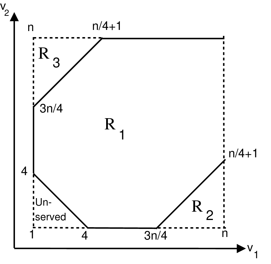
Figure 3 shows the allocation function of this lottery pricing. In particular, for is the set of valuations where lottery is bought. The probability mass of regions and together can be computed to be . The probability mass of region is . Therefore, the revenue of can be computed to be . This is a factor of higher than the optimal revenue for , or the revenue of any item pricing for .