跳到论文正文
W Papers独立论文阅读器 arXiv:1002.3760 论文正文 计算阅读时间 · 0%
引用这篇论文根据当前论文元数据生成,正式投稿前建议核对。


License: arXiv.org perpetual non-exclusive license
arXiv:1002.3760v6 [hep-th] 08 May 2011

AdS3 Vacua and RG Flows in Three Dimensional Gauged Supergravities

Preprint:  arXiv:1002.3760
Edi Gava Affiliation: INFN, Sezione di Trieste, Italy    Parinya Karndumri Affiliation: International School for Advanced Studies (SISSA), via Bonomea 265, 34136 Trieste, Italy    K. S. Narain Email: karndumr$@$sissa.it Email: narain$@$ictp.it Affiliation: The Abdus Salam International Centre for Theoretical Physics, Strada Costiera 11, 34100 Trieste, ItalyE-mail: , , Email: gava$@$ictp.it
Abstract: 

We study A​d​S3AdS_{3} supersymmetric vacua in N=4N=4 and N=8N=8, three dimensional gauged supergravities, with scalar manifolds (S​O​(4,4)S​O​(4)×S​O​(4))2(\frac{SO(4,4)}{SO(4)\times SO(4)})^{2} and S​O​(8,8)S​O​(8)×S​O​(8)\frac{SO(8,8)}{SO(8)\times SO(8)}, non-semisimple Chern-Simons gaugings S​O​(4)⋉𝐑6SO(4)\ltimes{\bf R}^{6} and (S​O​(4)⋉𝐑6)2(SO(4)\ltimes{\bf R}^{6})^{2}, respectively. These are in turn equivalent to S​O​(4)SO(4) and S​O​(4)×S​O​(4)SO(4)\times SO(4) Yang-Mills theories coupled to supergravity. For the N=4N=4 case, we study renormalization group flows between UV and IR A​d​S3AdS_{3} vacua with the same amount of supersymmetry: in one case, with (3,1) supersymmetry, we can find an analytic solution whereas in another, with (2,0) supersymmetry, we give a numerical solution. In both cases, the flows turn out to be v.e.v. flows, i.e. they are driven by the expectation value of a relevant operator in the dual S​C​F​T2SCFT_{2}. These provide examples of v.e.v. flows between two A​d​S3AdS_{3} vacua within a gauged supergravity framework.

Keywords: 
AdS/CFT correspondence, gauge-gravity correspondence

1 Introduction

Three dimensional gauged supergravities turn out to possess a very rich structure, and one reason to be interested in them, apart from their intrinsic geometrical elegance, is that they offer a convenient arena to discuss various aspects of A​d​S3/C​F​T2AdS_{3}/CFT_{2} correspondence, much in the same way the study of various backgrounds of five-dimensional gauged supergravity has been useful in uncovering interesting phenomena in the dual four dimensional Yang-Mills theory[1, 2, 3].
The construction of three dimensional, NN-extended, gauged supergravities has been worked out systematically for any N≤16N\leq 16 in [4] extending previous results on N=8,16N=8,16 obtained in [5, 6, 7]. When gauging isometries of the scalar manifold of the original, ungauged supergravity theory, one introduces gauge fields which have Chern-Simons kinetic terms and therefore do not represent propagating degrees of freedom. On the other hand, when reducing a higher dimensional supergravity theory down to three dimensions, which is the instance we are interested in, one generically obtains gauge-fields with Yang-Mills like kinetic terms. The apparent puzzle was solved in [4] and [8] and has to do with the duality between gauge fields and scalars in three dimensional space-time: more precisely, it has been shown there that, if the gauge group is not semisimple, but contains nilpotent shift symmetries, i.e. it is of the form G⋉𝐑dim​GG\ltimes{\bf R}^{{\rm dim}G}, then one can integrate out half of the 2​dim​G2\,{\rm dim}G Chern-Simons gauge fields to produce a Yang-Mills action for the remaining ones. At the same time, dim​G{\rm dim}G scalars can be set to zero by using the shift symmetries. In other words, one trades scalars with vectors and, of course, the number of physical degrees of freedom is unchanged. This mechanism has been employed, for example, in [9] for N=8N=8, where it has been shown that a gauging by S​O​(4)⋉𝐑6SO(4)\ltimes{\bf R}^{6} indeed reproduces, at the N=8N=8 point in the scalar manifold, the Kaluza-Klein spectrum of the six-dimensional (2,0) supergravity on A​d​S3×S3AdS_{3}\times S^{3}[10]. The latter is the background one obtains by taking the near horizon geometry of a D1-D5 system of type IIB theory on K​3K3 or T4T^{4}, corresponding to a C​F​T2CFT_{2} with (4,4) supersymmetry.
In this paper, we analyze two examples of gauged supergravities with non-semisimple gauging, with N=4N=4 and N=8N=8 supersymmetry, whose scalar manifolds take the forms of (S​O​(4,4)S​O​(4)×S​O​(4))2(\frac{SO(4,4)}{SO(4)\times SO(4)})^{2} and S​O​(8,8)S​O​(8)×S​O​(8)\frac{SO(8,8)}{SO(8)\times SO(8)}, respectively. As for the gauging, we will consider gauge groups S​O​(4)⋉𝐑6SO(4)\ltimes{\bf R}^{6} and (S​O​(4)⋉𝐑6)2(SO(4)\ltimes{\bf R}^{6})^{2}, respectively. These turn out to be subgroups of the isometry groups which can be gauged consistently with supersymmetry, as will be shown.
We will study supersymmetric A​d​S3AdS_{3} vacua in both of these theories, with various amount of preserved supersymmetries. In the N=4N=4 case, we will be able to study the flow between different vacua with different cosmological constants but the same amount of supersymmetry. Quite remarkably, we will be able to find an analytic flow solution between vacua with (3,1) supersymmetry involving two active scalar fields. For the case of flow between (2,0) vacua which involves three active scalars, we will discuss a numerical flow solution. The flows turn out to be v.e.v. flows driven by vacuum expectation values of some operators in the UV. Examples of v.e.v. flows are known in four dimensional super-conformal field theories, in particular in N=2N=2 SCFT, where they have been studied using Seiberg-Witten solution in connection with the Argyres-Douglas fixed points[11, 12, 13]. To the best of our knowledge, these are the first examples of v.e.v. flows between two A​d​SAdS vacua in a gauged supergravity context.
From the higher dimensional perspective, the case with N=8N=8 supersymmetry (or better its maximally symmetric vacuum) is related to the brane configuration in type IIB theory whose near horizon geometry is A​d​S3×S3×S3×S1AdS_{3}\times S^{3}\times S^{3}\times S^{1} [14], dual to a C​F​T2CFT_{2} with “large” (4,4)(4,4) superconformal algebra[15, 16]. For the N=4N=4 case, which has a (4,0) vacuum, the ten dimensional interpretation is far less clear. It could be related to some warped or orbifolded versions of the previous case. It would be interesting to establish this.
The paper is organized as follows. In section 2, we review the features of three dimensional gauged supergravity in the case where the target manifold is a symmetric space. In section 3, we specialize at the N=4N=4 theory and describe the vacua we found. In section 4, we discuss the analytic flow solutions between (3,1) vacua, and numerical flow solution between (2,0) vacua. In section 5, we move to the N=8N=8 case and describe the vacua we obtained. The algebraic manipulations and the numerical solution of the BPS differential equations have been performed with the help of Mathematica. In section 6, we make some conclusions.

2 Three Dimensional Gauged Supergravity

In this section, we review the basic features of 3 dimensional, N-extended, gauged supergravity, following the N-covariant formulation given in reference [4]. We will restrict our discussion to the case where the scalar manifold is a symmetric space G/HG/H, although for N<5N<5 there are more general possibilities. Before gauging, the propagating bosonic sector of the theory is described by a non-linear sigma model whose target manifold is G/HG/H, where HH is a maximal compact subgroup of GG. Thus there are scalar fields ϕi​(x)\phi^{i}(x), i=1,…,dim​G/Hi=1,\dots,{\rm dim}\,G/H, which are coordinates of G/HG/H. The subgroup HH of GG contains the R-symmetry group S​O​(N)SO(N). Gauging proceeds by introducing Chern-Simons gauge fields AμℳA_{\mu}^{\mathcal{M}} in the adjoint representation of a subgroup G′G^{\prime} of the isometry group GG, whose embedding in GG is specified by a gauge invariant, symmetric embedding tensor Θℳ​𝒩\Theta_{\mathcal{M}\mathcal{N}}, with indices running over the Lie algebra of the gauged subgroup. Supersymmetry severely restricts the allowed gauged subgroup, and correspondingly the tensor Θ\Theta, as we will see in the following. For the reasons explained in the introduction, we will be interested in non-semisimple gaugings, where the gauged subgroup is a semi-direct product of a semisimple factor G0G_{0} and an abelian factor T=𝐑dim​G0T={\bf R}^{{\rm dim}G_{0}}, G′=G0⋉TG^{\prime}=G_{0}\ltimes T, with the latter transforming in the adjoint representation of G0G_{0}.
Let us now introduce the basic data which allow us to construct the gauged supergravity theory in the symmetric space case: recall that by G/HG/H we mean the manifold of right cosets, where HH elements h⁡(x)h(x) act by right multiplication on the GG-valued matrix L​(ϕi​(x))L(\phi^{i}(x)). The generators of GG decompose into {tℳ}={XI​J,Xα,YA}\{t^{\mathcal{M}}\}=\{X^{IJ},X^{\alpha},Y^{A}\}. XI​JX^{IJ} generate S​O​(N)SO(N), and XαX^{\alpha} generate a group H′H^{\prime} commuting with S​O​(N)SO(N). YAY^{A} are the non-compact generators of GG. The isometry group is defined by the left action of GG elements on the coset G/HG/H. The geometry of G/HG/H is encoded in the Lie algebra valued one-forms L−1​∂iLL^{-1}\partial_{i}L and in L−1​tℳ​LL^{-1}t^{\mathcal{M}}L, through the following expansions over Lie algebra generators:

L−1​∂iL\displaystyle L^{-1}\partial_{i}L =\displaystyle= 12​QiI​J​XI​J+Qiα​Xα+eiA​YA,\displaystyle\frac{1}{2}Q^{IJ}_{i}X^{IJ}+Q^{\alpha}_{i}X^{\alpha}+e^{A}_{i}Y^{A},
L−1​tℳ​L\displaystyle L^{-1}t^{\mathcal{M}}L =\displaystyle= 12​𝒱ℳ​I​J​XI​J+𝒱αℳ​Xα+𝒱Aℳ​YA.\displaystyle\frac{1}{2}\mathcal{V}^{\mathcal{M}IJ}X^{IJ}+\mathcal{V}^{\mathcal{M}}_{\phantom{a}\alpha}X^{\alpha}+\mathcal{V}^{\mathcal{M}}_{\phantom{a}A}Y^{A}. (1)

The eiAe^{A}_{i} are vielbeins which determine the invariant metric gi​j=eiA​ejB​δA​Bg_{ij}=e^{A}_{i}e^{B}_{j}\delta_{AB} of G/HG/H. The QQ’s are composite HH-connections, and the 𝒱\mathcal{V}’s give the Killing vectors, 𝒱ℳ​i=gi​j​ejA​𝒱Aℳ\mathcal{V}^{\mathcal{M}i}=g^{ij}e^{A}_{j}\mathcal{V}^{\mathcal{M}}_{\phantom{a}A}. Pulling back on space-time and covariantizing with respect to the gauge action of G′G^{\prime} from the right, we define:

L−1​Dμ​L=12​QμI​J​XI​J+Qμα​Xα+eμA​YA.L^{-1}D_{\mu}L=\frac{1}{2}Q^{IJ}_{\mu}X^{IJ}+Q^{\alpha}_{\mu}X^{\alpha}+e^{A}_{\mu}Y^{A}. (2)

Here DμL=(∂μ+Θℳ​𝒩Aμℳt𝒩)LD_{\mu}L=(\partial_{\mu}+\Theta_{\mathcal{M}\mathcal{N}}A_{\mu}^{\mathcal{M}}t^{\mathcal{N}})L is a space-time covariant derivative and it is understood that the gauge coupling constant is contained in Θ\Theta. Thus the full gauge symmetry of the theory is L⁡(x)→g′​(x)​L​(x)​h​(x)L(x)\rightarrow g^{\prime}(x)L(x)h(x), where g′∈G′g^{\prime}\in G^{\prime}. The eμAe^{A}_{\mu}’s give the covariant kinetic term for scalars,

ℒkin=14​g​gμ​ν​eμA​eνB​δA​B.{\mathcal{L}}_{\textrm{kin}}=\frac{1}{4}\sqrt{g}g^{\mu\nu}e^{A}_{\mu}e^{B}_{\nu}\delta_{AB}. (3)

The Lagrangian for gauge fields is of Chern-Simons type:

ℒC​S=14​ϵμ​ν​ρ​Aμℳ​Θℳ​𝒩​(∂νAρ𝒩+13​f𝒬𝒩​𝒫​Θ𝒫​ℒ​Aνℒ​Aρ𝒬),{\mathcal{L}}_{CS}=\frac{1}{4}\epsilon^{\mu\nu\rho}A_{\mu}^{\mathcal{M}}\Theta_{{\mathcal{M}}{\mathcal{N}}}(\partial_{\nu}A_{\rho}^{\mathcal{N}}+\frac{1}{3}f^{{\mathcal{N}}{\mathcal{P}}}_{\mathcal{Q}}\Theta_{{\mathcal{P}}{\mathcal{L}}}A_{\nu}^{\mathcal{L}}A_{\rho}^{\mathcal{Q}}), (4)

where f𝒬𝒩​𝒫f^{{\mathcal{N}}{\mathcal{P}}}_{\mathcal{Q}} are the structure constants of G′G^{\prime}.
As it has been shown in [4] and in more detail in [8], in the non-semisimple case where G′=G0⋉TG^{\prime}=G_{0}\ltimes T, the Chern-Simons action for G′G^{\prime} gauge fields is equivalent to a Yang-Mills plus Chern-Simons action for gauge fields transforming under the semisimple part G0G_{0}. The point is that gauge invariance implies that the indices of Θℳ​𝒩\Theta_{{\mathcal{M}}{\mathcal{N}}} cannot be both along the G0G_{0} direction and this allows to integrate the gauge fields carrying G0G_{0} indices, producing a Yang-Mills action for gauge fields carrying TT indices, which transform in the usual way under G0G_{0}. At the same time, one can use the shift gauge symmetry to remove dim​G0{\rm dim}\,G_{0} scalars from the action.
A class of tensors that will play important role in our analysis are the two-form S​O​(N)SO(N) generators, fi​jI​Jf^{IJ}_{ij}, which originate from the existence of N−1N-1 hermitean almost complex structures fjP​if^{Pi}_{j}, P=1,…,N−1P=1,\dots,N-1, on the scalar manifold. The existence of the latter is implied by the existence of NN supersymmetries. They are vector valued one-forms obeying a Clifford algebra relation and therefore are essentially γ\gamma-matrices of S​O​(N)SO(N). With their commutators one constructs S​O​(N)SO(N) generators fi​jI​Jf^{IJ}_{ij}, which in our case can be expressed as:

fi​jI​J=−ΓA​BI​J​eiA​ejB,f^{IJ}_{ij}=-\Gamma^{IJ}_{AB}e^{A}_{i}e^{B}_{j}, (5)

with ΓA​BI​J\Gamma^{IJ}_{AB} properly normalized generators in the spinor representation of S​O​(N)SO(N). Let us now specialize at the N=4N=4 and N=8N=8 cases. In the latter case, one proves that the allowed symmetric spaces are of the form S​O​(8,k)S​O​(8)×S​O​(k)\frac{SO(8,k)}{SO(8)\times SO(k)}, and in fact we will restrict our analysis to k=8k=8. For N=4N=4, the scalar manifold can actually be locally the product of two quaternionic manifolds, and even restricting to the symmetric space cases, this allows a finite number of different possibilities, but we will restrict the analysis to the quaternionic symmetric space S​O​(4,4)S​O​(4)×S​O​(4)\frac{SO(4,4)}{SO(4)\times SO(4)}.
With the data introduced above, namely the embedding tensor Θ\Theta and the 𝒱\mathcal{V}’s, we define the T-tensors:

TI​J,K​L\displaystyle T^{IJ,KL} ≡\displaystyle\equiv 𝒱ℳ​I​J​Θℳ​𝒩​𝒱𝒩​K​L,TI​J​i≡𝒱ℳ​I​J​Θℳ​𝒩​𝒱𝒩​i,\displaystyle\mathcal{V}^{\mathcal{M}IJ}\Theta_{\mathcal{M}\mathcal{N}}\mathcal{V}^{\mathcal{N}KL},\qquad T^{IJi}\equiv\mathcal{V}^{\mathcal{M}IJ}\Theta_{\mathcal{M}\mathcal{N}}\mathcal{V}^{\mathcal{N}i},
Ti​j\displaystyle T^{ij} ≡\displaystyle\equiv 𝒱ℳ​i​Θℳ​𝒩​𝒱𝒩​j,Tαi≡𝒱αℳ​Θℳ​𝒩​𝒱𝒩​i,\displaystyle\mathcal{V}^{\mathcal{M}i}\Theta_{\mathcal{M}\mathcal{N}}\mathcal{V}^{\mathcal{N}j},\qquad T^{i}_{\phantom{a}\alpha}\equiv\mathcal{V}^{\mathcal{M}}_{\phantom{a}\alpha}\Theta_{\mathcal{M}\mathcal{N}}\mathcal{V}^{\mathcal{N}i},
Tα​β\displaystyle T_{\alpha\beta} ≡\displaystyle\equiv 𝒱αℳ​Θℳ​𝒩​𝒱βℳ,TαI​J≡𝒱ℳ​I​J​Θℳ​𝒩​𝒱α𝒩.\displaystyle\mathcal{V}^{\mathcal{M}}_{\phantom{a}\alpha}\Theta_{\mathcal{M}\mathcal{N}}\mathcal{V}^{\mathcal{M}}_{\phantom{a}\beta},\qquad T^{IJ}_{\phantom{ab}\alpha}\equiv\mathcal{V}^{\mathcal{M}IJ}\Theta_{\mathcal{M}\mathcal{N}}\mathcal{V}^{\mathcal{N}}_{\phantom{a}\alpha}. (6)

The fundamental consistency constraint on the gauging, implied by supersymmetry, can be expressed through the following identity:

TI​J,K​L=T[I​J,K​L]−4N−2δI[KTL]M,MJ−2(N−1)​(N−2)δI[KδL]JTM​N,M​N,T^{IJ,KL}=T^{[IJ,KL]}-\frac{4}{N-2}\delta^{I[K}T^{L]M,MJ}-\frac{2}{(N-1)(N-2)}\delta^{I[K}\delta^{L]J}T^{MN,MN}, (7)

or equivalently,

ℙ⊞​TI​J,K​L=0\mathbb{P}_{\boxplus}T^{IJ,KL}=0 (8)

which means that the representation ⊞\boxplus of S​O​(N)SO(N) is projected out. The scalar potential of the theory can be expressed in terms of the tensors:

A1I​J\displaystyle A_{1}^{IJ} =\displaystyle= −4N−2​TI​M,J​M+2(N−1)​(N−2)​δI​J​TM​N,M​N,\displaystyle-\frac{4}{N-2}T^{IM,JM}+\frac{2}{(N-1)(N-2)}\delta^{IJ}T^{MN,MN},
A2​jI​J\displaystyle A_{2j}^{IJ} =\displaystyle= 2N​TjI​J+4N⁡(N−2)​fjM⁡(I​mCLOSE​TmOPENJ)​M+2N​(N−1)​(N−2)​δI​J​fjK​L​m​TmK​L.\displaystyle\frac{2}{N}T^{IJ}_{\phantom{as}j}+\frac{4}{N(N-2)}f^{M(Im}_{\phantom{as}j}T^{J)M}_{\phantom{as}m}+\frac{2}{N(N-1)(N-2)}\delta^{IJ}f^{KL\phantom{a}m}_{\phantom{as}j}T^{KL}_{\phantom{as}m}. (9)

Supersymmetry implies a quadratic identity involving A1A_{1} and A2A_{2} :

2​A1I​K​A1K​J−N​A2I​K​i​A2​iJ​K=δI​JN​(2​A1K​L​A1K​L−N​A2K​L​i​A2​iK​L),2A_{1}^{IK}A_{1}^{KJ}-NA_{2}^{IKi}A_{2i}^{JK}=\frac{\delta^{IJ}}{N}(2A_{1}^{KL}A_{1}^{KL}-NA_{2}^{KLi}A_{2i}^{KL}), (10)

which offers a non-trivial check on the consistency of the construction. The scalar potential is given by:

V=−4N​g​(A1I​J​A1I​J−12​N​gi​j​A2​iI​J​A2​jI​J).V=-\frac{4}{N}\sqrt{g}(A_{1}^{IJ}A_{1}^{IJ}-\frac{1}{2}Ng^{ij}A_{2i}^{IJ}A_{2j}^{IJ}). (11)

Since Θ\Theta’s are linear in the gauge couplings, VV depends quadratically on them. The other piece of information we will need is given by the supersymmetry variations of the matter fermions χ\chi and the gravitinos ψμI\psi^{I}_{\mu}. For the former, in order to use the S​O​(N)SO(N) covariant notations, we extend the fermion fields χi\chi^{i} to an overcomplete set χi​I\chi^{iI} defined by,[4],

χi​I=(χi,fjP​i​χj).\chi^{iI}=(\chi^{i},f^{Pi}_{j}\chi^{j}). (12)

The Lagrangian and supersymmetry transformation rules can be expressed in a form that no longer depends explicitly on the almost complex structures. The fields χi​I\chi^{iI} have to satisfy the projection constraint

χi​I=ℙJ​jI​i​χj​J≡1N​(δI​J​δji−fjI​J​i)​χj​J.\chi^{iI}=\mathbb{P}^{Ii}_{Jj}\chi^{jJ}\equiv\frac{1}{N}(\delta^{IJ}\delta^{i}_{j}-f^{IJi}_{j})\chi^{jJ}. (13)

Omitting terms which are of higher order in the fermionic fields, the supersymmetry transformations which are relevant for us are given by:

δ​ψμI\displaystyle\delta\psi^{I}_{\mu} =\displaystyle= 𝒟μ​ϵI+A1I​J​γμ​ϵJ,\displaystyle\mathcal{D}_{\mu}\epsilon^{I}+A_{1}^{IJ}\gamma_{\mu}\epsilon^{J},
δ​χi​I\displaystyle\delta\chi^{iI} =\displaystyle= 12​(δI​J​𝟏−fI​J)ji​𝒟/ϕj​ϵJ−N​A2J​I​i​ϵJ,\displaystyle\frac{1}{2}(\delta^{IJ}\mathbf{1}-f^{IJ})^{i}_{\phantom{a}j}{\mathcal{D}{\!\!\!\!/}}\phi^{j}\epsilon^{J}-NA_{2}^{JIi}\epsilon^{J}, (14)

where

𝒟μ​ϵI\displaystyle\mathcal{D}_{\mu}\epsilon^{I} =\displaystyle= (∂μ+12ωμaγa)ϵI+∂μϕiQiI​JϵJ+Θℳ​𝒩Aμℳ𝒱𝒩​I​JϵJ,\displaystyle(\partial_{\mu}+\frac{1}{2}\omega^{a}_{\phantom{a}\mu}\gamma_{a})\epsilon^{I}+\partial_{\mu}\phi^{i}Q_{i}^{IJ}\epsilon^{J}+\Theta_{\mathcal{M}\mathcal{N}}A_{\mu}^{\mathcal{M}}\mathcal{V}^{\mathcal{N}IJ}\epsilon^{J},
𝒟μ​ϕi\displaystyle\mathcal{D}_{\mu}\phi^{i} =\displaystyle= ∂μϕi+Aμℳ​𝒱𝒩​i​Θℳ​𝒩,\displaystyle\partial_{\mu}\phi^{i}+A_{\mu}^{\mathcal{M}}\mathcal{V}^{\mathcal{N}i}\Theta_{\mathcal{M}\mathcal{N}}, (15)

and ωμa\omega^{a}_{\mu} is the 3-dimensional spin connection constructed with the dreibein eμae^{a}_{\mu}. As shown in [4], assuming a maximally symmetric space-time (in particular A​d​S3AdS_{3}), the supersymmetric critical points of the potential are given by the two equivalent conditions on spinors ϵI\epsilon^{I}:

A2​iJ​I​ϵJ\displaystyle A_{2i}^{JI}\epsilon^{J} =\displaystyle= 0\displaystyle 0
andA1I​K​A1K​J​ϵJ\displaystyle\textrm{and}\qquad A_{1}^{IK}A_{1}^{KJ}\epsilon^{J} =\displaystyle= −V04​ϵI=1N​(A1I​J​A1I​J−12​N​gi​j​A2​iI​J​A2​iI​J)​ϵI,\displaystyle-\frac{V_{0}}{4}\epsilon^{I}=\frac{1}{N}(A_{1}^{IJ}A_{1}^{IJ}-\frac{1}{2}Ng^{ij}A_{2i}^{IJ}A_{2i}^{IJ})\epsilon^{I}, (16)

where V0V_{0} is the potential at the critical point. The equivalence of the two statements follows from the quadratic identity (10) involving A1A_{1} and A2A_{2}. This result says that the preserved supersymmetries correspond to the eigenvalues of A1I​JA_{1}^{IJ} which equal ±−V04\pm\sqrt{\frac{-V_{0}}{4}}, since in our normalization −V0=R−2-V_{0}=R^{-2}, where RR is the radius of A​d​S3AdS_{3}. More in detail, let us choose A​d​S3AdS_{3} coordinates r,x0,x1r,x_{0},x_{1}, and metric d​s2=d​r2+e2​r/R​(−d​x02+d​x12)ds^{2}=dr^{2}+e^{2r/R}(-dx_{0}^{2}+dx_{1}^{2}). From the previous remarks, it follows that for each eigenvector v±Iv^{I}_{\pm} of A1I​JA_{1}^{IJ}, with eigenvalue ±−V04\pm\sqrt{\frac{-V_{0}}{4}}, if we form the spinor ϵ±I=ϵ±⊗v±I\epsilon^{I}_{\pm}=\epsilon_{\pm}\otimes v^{I}_{\pm}, then the BPS condition for the gravitino variation (14) becomes identical to the Killing spinor equation for ϵ±\epsilon_{\pm} on A​d​S3AdS_{3} i.e. 𝒟μ​ϵ±=±12​R​γμ​ϵ±\mathcal{D}_{\mu}\epsilon_{\pm}=\pm\frac{1}{2R}\gamma_{\mu}\epsilon_{\pm}. Using the explicit expression for the spin connection for the above metric, one can see that one solution to this equation is an x0,x1x_{0},x_{1}-independent spinor obeying γr​ϵ±=±ϵ±\gamma^{r}\epsilon_{\pm}=\pm\epsilon_{\pm}, where γr\gamma^{r} is the flat gamma matrix. This corresponds to a left (right) Poincare’ supersymmetry in the boundary CFT. The other solution gives rise to the superconformal charge in the boundary CFT, has a non-trivial x0,x1x_{0},x_{1} dependence and is constructed with a constant spinor obeying the opposite γr\gamma^{r} projection condition.
Therefore, it is convenient to classify the critical points by presenting their preserved supersymmetries in the form of (N+,N−)(N_{+},N_{-}) corresponding to the N+N_{+} and N−N_{-} positive and negative eigenvalues of A1I​JA_{1}^{IJ} whose modulus equals −V04\sqrt{\frac{-V_{0}}{4}}. These coincide with the number of left-(right-) moving Poincare’ supersymmetries of the dual S​C​F​T2SCFT_{2}. Of course the total number of supersymmetries is doubled by the inclusion of the superconformal ones.
To summarize, the procedure of finding supersymmetric vacua is the following. From (16), we look for the Killing spinors ϵI\epsilon^{I} which are annihilated by some of the A2​iJ​IA_{2i}^{JI}. At the same time, ϵI\epsilon^{I} must also be the eigenvector of A1I​JA_{1}^{IJ}. Clearly, maximal supersymmetric vacua are annihilated by all of the components of A2​iJ​IA_{2i}^{JI}, and ϵI\epsilon^{I} is an eigenvector of A1I​JA_{1}^{IJ} for all directions II. The ϵI\epsilon^{I} characterizing partially supersymmetric vacua will be an eigenvector of A1I​JA_{1}^{IJ} for certain directions labeled by some values of II, and will be annihilated only by the A2​iJ​IA_{2i}^{JI} in the corresponding directions. We also find many supersymmetric vacua with V0=0V_{0}=0, and there might be non-supersymmetric A​d​S3AdS_{3} vacua as well. However, in this work, we will not discuss them.

3 Vacua of the N=4N=4 Theory

The target space in our case is the product of two quaternionic manifolds, that we take to be S​O​(4,4)/S​O​(4)×S​O​(4)SO(4,4)/SO(4)\times SO(4). A convenient (redundant) parametrization of cosets is given by the following SO(4,4) group element

Li=12​(Xi+eitYi+eit−Xi+eiteit−Yi),L_{i}=\frac{1}{2}\left(\begin{array}[]{cc}X_{i}+e^{t}_{i}&Y_{i}+e^{t}_{i}\\ -X_{i}+e^{t}_{i}&e^{t}_{i}-Y_{i}\\ \end{array}\right), (17)

where i=1,2i=1,2 refers to the two spaces. eie_{i} is a 4×44\times 4 matrix in GL(4,R), Xi=Ei+Bi​eitX_{i}=E_{i}+B_{i}e_{i}^{t}, Yi=−Ei+Bi​eitY_{i}=-E_{i}+B_{i}e_{i}^{t}. BiB_{i} is an antisymmetric 4×44\times 4 matrix, and Ei=ei−1E_{i}=e_{i}^{-1}. The inverse of LiL_{i} is

Li−1=12​(Xit+eiXit−ei−Yit−eiei−Yit).L^{-1}_{i}=\frac{1}{2}\left(\begin{array}[]{cc}X^{t}_{i}+e_{i}&X^{t}_{i}-e_{i}\\ -Y^{t}_{i}-e_{i}&e_{i}-Y_{i}^{t}\\ \end{array}\right). (18)

One can eliminate 6 of the 22 parameters in LL by using the right action of the diagonal S​O​(4)SO(4) action, for example by bringing eie_{i} into an upper triangular form. The following Lie algebra elements,

t𝒜=(a00a)tℬ=(bb−b−b)t^{\mathcal{A}}=\left(\begin{array}[]{cc}a&0\\ 0&a\\ \end{array}\right)\qquad t^{\mathcal{B}}=\left(\begin{array}[]{cc}b&b\\ -b&-b\\ \end{array}\right) (19)

where all entries are 4×44\times 4 antisymmetric blocks, together with an identical copy for the second space, will be gauged. In other words, the semisimple part of the gauge group will be the diagonal S​O​(4)DSO(4)_{D} in the (S​O​(4))4(SO(4))^{4} of the product (S​O​(4,4)S​O​(4)×S​O​(4))2(\frac{SO(4,4)}{SO(4)\times SO(4)})^{2}, corresponding to generators t𝒜t^{\mathcal{A}}. On the other hand, the nilpotent generators, tℬt^{\mathcal{B}}, generate diagonal shift symmetries B1,2→B1,2+2​bB_{1,2}\rightarrow B_{1,2}+2b. Also, it is clear that the ℬ\mathcal{B}-generators transform in the adjoint representation with respect to the diagonal S​O​(4)SO(4). For aa and bb, we can take a basis of antisymmetric matrices given by JI​J=εI​J−εJ​IJ^{IJ}=\varepsilon^{IJ}-\varepsilon^{JI}, with (εI​J)K​L=δI​K​δJ​L(\varepsilon^{IJ})_{KL}=\delta_{IK}\delta_{JL}. Similarly, we can use the following basis for the 16 non-compact generators of S​O​(4,4)SO(4,4):

Ya​b=(0εa​b(εt)a​b0).Y^{ab}=\left(\begin{array}[]{cc}0&\varepsilon^{ab}\\ (\varepsilon^{t})^{ab}&0\\ \end{array}\right). (20)

Since in the present case both the R symmetry group and the gauge group are S​O​(4)SO(4), it is convenient to split the corresponding Lie algebras generators into self-dual and anti-self-dual components J+J_{+} and J−J_{-} respectively:

J+I​J=JI​J+12​ϵI​J​K​L​JK​LandJ−I​J=JI​J−12​ϵI​J​K​L​JK​LJ_{+}^{IJ}=J^{IJ}+\frac{1}{2}\epsilon^{IJKL}J^{KL}\qquad\textrm{and}\qquad J_{-}^{IJ}=J^{IJ}-\frac{1}{2}\epsilon^{IJKL}J^{KL} (21)

which are S​U​(2)+SU(2)_{+} and S​U​(2)−SU(2)_{-} generators in the S​O​(4)=S​U​(2)+⊕S​U​(2)−SO(4)=SU(2)_{+}\oplus SU(2)_{-} Lie algebra decomposition. We will adopt this decomposition both for 𝒜\mathcal{A}- and ℬ\mathcal{B}-type generators. Correspondingly, the two-forms tensors fI​Jf^{IJ} introduced in the previous section have, say, self-dual components on the first quaternionic space and anti-self-dual components on the second. In our formalism and in a flat basis, they can be expressed as:

f±I​Ja​b,c​d=Tr​((εt)a​b​J±I​J​εc​d).{f^{IJ}_{\pm}}_{ab,cd}=\textrm{Tr}((\varepsilon^{t})^{ab}J_{\pm}^{IJ}\varepsilon^{cd}). (22)

At this stage, we can proceed to construct the supergravity theory with the gauging of S​O​(4)⋉𝐑6SO(4)\ltimes{\bf R}^{6} and in particular, verify its consistency, along the lines reviewed in the previous section. As explained there, the main ingredients are given by the tensors A1A_{1} and A2A_{2}, which determine the scalar potential and the supersymmetry variations of the fermionic fields. They are constructed through the TT-tensors, which in turn are obtained by uplifting the embedding tensor Θℳ​𝒩\Theta_{\mathcal{M}\mathcal{N}} into GG by using 𝒱𝒫ℳ{\mathcal{V}}^{\mathcal{M}}_{\mathcal{P}}, with 𝒫\mathcal{P} running over the generators of GG corresponding to the R-symmetries 𝒫=I​J\mathcal{P}=IJ, and the non-compact coset directions 𝒫=a​b\mathcal{P}=ab in the first and second space. We give in the Appendix A expressions for the relevant components of 𝒱\mathcal{V}.
Gauge invariance restricts the Θ\Theta tensors to have components, Θ𝒜​ℬ\Theta_{\mathcal{A}\mathcal{B}} and Θℬ​ℬ\Theta_{\mathcal{B}\mathcal{B}}, which are proportional to the S​O​(4)SO(4) Killing form, schematically δ𝒜​ℬ\delta_{\mathcal{A}\mathcal{B}} and δℬ​ℬ\delta_{\mathcal{B}\mathcal{B}}, respectively. The proportionality constants are gauge couplings, and, of course, we should specify here to which of the four S​U​(2)SU(2)’s the 𝒜\mathcal{A}, ℬ\mathcal{B} indices belong. Therefore, a priori we expect four couplings g1​s,g1​a,g2​s,g_{1s},g_{1a},g_{2s}, and g2​ag_{2a}. The aa and ss labels indicate the self-dual and anti-self-dual S​U​(2)SU(2), respectively, and 1 refers to the 𝒜​ℬ\mathcal{A}\mathcal{B} couplings whereas 2 refers to the ℬ​ℬ\mathcal{B}\mathcal{B} ones.
With this notation and with the meaning of 𝒱\mathcal{V} indices explained in the Appendix A, the TT-tensors turn out to be:

TL​J,M​K\displaystyle T^{LJ,MK} =\displaystyle= g1​s​(𝒱+aL​J,P​Q​𝒱+bM​K,P​Q+𝒱+bL​J,P​Q​𝒱+aM​K,P​Q)+g1​a​(𝒱−aL​J,P​Q​𝒱−bM​K,P​QCLOSE\displaystyle g_{1s}(\mathcal{V}_{\textrm{+a}}^{LJ,PQ}\mathcal{V}_{\textrm{+b}}^{MK,PQ}+\mathcal{V}_{\textrm{+b}}^{LJ,PQ}\mathcal{V}_{\textrm{+a}}^{MK,PQ})+g_{1a}(\mathcal{V}_{-\textrm{a}}^{LJ,PQ}\mathcal{V}_{-\textrm{b}}^{MK,PQ}
OPEN+𝒱−bL​J,P​Q​𝒱−aM​K,P​Q)+g2​s​𝒱+bL​J,P​Q​𝒱+bM​K,P​Q+g2​a​𝒱−bL​J,P​Q​𝒱−bM​K,P​Q,\displaystyle+\mathcal{V}_{-\textrm{b}}^{LJ,PQ}\mathcal{V}_{-\textrm{a}}^{MK,PQ})+g_{2s}\mathcal{V}_{\textrm{+b}}^{LJ,PQ}\mathcal{V}_{\textrm{+b}}^{MK,PQ}+g_{2a}\mathcal{V}_{-\textrm{b}}^{LJ,PQ}\mathcal{V}_{-\textrm{b}}^{MK,PQ},
T1a​bL​J\displaystyle{T_{1}}^{LJ}_{ab} =\displaystyle= g1​s​(𝒱+aL​J,P​Q​𝒱+1ba​bP​Q+𝒱+bL​J,P​Q​𝒱+1aa​bP​Q)+g1​a​(𝒱−aL​J,P​Q​𝒱−1ba​bP​QCLOSE\displaystyle g_{1s}(\mathcal{V}_{\textrm{+a}}^{LJ,PQ}{\mathcal{V}_{\textrm{+1b}}}^{PQ}_{ab}+\mathcal{V}_{\textrm{+b}}^{LJ,PQ}{\mathcal{V}_{\textrm{+1a}}}^{PQ}_{ab})+g_{1a}(\mathcal{V}_{-\textrm{a}}^{LJ,PQ}{\mathcal{V}_{-\textrm{1b}}}^{PQ}_{ab}
OPEN+𝒱−bL​J,P​Q​𝒱−1aa​bP​Q)+g2​s​𝒱+bL​J,P​Q​𝒱+1ba​bP​Q+g2​a​𝒱−bL​J,P​Q​𝒱−1ba​bP​Q,\displaystyle+\mathcal{V}_{-\textrm{b}}^{LJ,PQ}{\mathcal{V}_{-\textrm{1a}}}^{PQ}_{ab})+g_{2s}\mathcal{V}_{\textrm{+b}}^{LJ,PQ}{\mathcal{V}_{\textrm{+1b}}}^{PQ}_{ab}+g_{2a}\mathcal{V}_{-\textrm{b}}^{LJ,PQ}{\mathcal{V}_{-\textrm{1b}}}^{PQ}_{ab},
T2a​bL​J\displaystyle{T_{2}}^{LJ}_{ab} =\displaystyle= g1​s​(𝒱+aL​J,P​Q​𝒱+2ba​bP​Q+𝒱+bL​J,P​Q​𝒱+2aa​bP​Q)+g1​a​(𝒱−aL​J,P​Q​𝒱−2ba​bP​QCLOSE\displaystyle g_{1s}(\mathcal{V}_{\textrm{+a}}^{LJ,PQ}{\mathcal{V}_{\textrm{+2b}}}^{PQ}_{ab}+\mathcal{V}_{\textrm{+b}}^{LJ,PQ}{\mathcal{V}_{\textrm{+2a}}}^{PQ}_{ab})+g_{1a}(\mathcal{V}_{-\textrm{a}}^{LJ,PQ}{\mathcal{V}_{-\textrm{2b}}}^{PQ}_{ab} (23)
OPEN+𝒱−bL​J,P​Q​𝒱−2aa​bP​Q)+g2​s​𝒱+bL​J,P​Q​𝒱+2ba​bP​Q+g2​a​𝒱−bL​J,P​Q​𝒱−2ba​bP​Q.\displaystyle+\mathcal{V}_{-\textrm{b}}^{LJ,PQ}{\mathcal{V}_{-\textrm{2a}}}^{PQ}_{ab})+g_{2s}\mathcal{V}_{\textrm{+b}}^{LJ,PQ}{\mathcal{V}_{\textrm{+2b}}}^{PQ}_{ab}+g_{2a}\mathcal{V}_{-\textrm{b}}^{LJ,PQ}{\mathcal{V}_{-\textrm{2b}}}^{PQ}_{ab}.

It turns out that the consistency requirement on TI​J,K​LT^{IJ,KL}, discussed in the previous section, requires g2​a=−g2​sg_{2a}=-g_{2s}. Moreover, we find it is convenient for the subsequent analysis to redefine the couplings from g1​sg_{1s}, g1​ag_{1a} to gng_{n}, gpg_{p} as follows:

g1​s=gp+gnandg1​a=gp−gn.g_{1s}=g_{p}+g_{n}\qquad\textrm{and}\qquad g_{1a}=g_{p}-g_{n}. (24)

Now, we study various vacua of this theory. We begin by choosing an ansatz for the coset LL. We have two spaces. We set B1=B2=0B_{1}=B_{2}=0 and choose diagonal eie_{i}’s:

e1=(a10000a20000a30000a4)ande2=(b10000b20000b30000b4).e_{1}=\left(\begin{array}[]{cccc}a_{1}&0&0&0\\ 0&a_{2}&0&0\\ 0&0&a_{3}&0\\ 0&0&0&a_{4}\\ \end{array}\right)\qquad\textrm{and}\qquad e_{2}=\left(\begin{array}[]{cccc}b_{1}&0&0&0\\ 0&b_{2}&0&0\\ 0&0&b_{3}&0\\ 0&0&0&b_{4}\\ \end{array}\right). (25)

Notice that the shift gauge symmetry would allow us to set one of the two BB’s to zero and the left S​O​(4)SO(4) gauge symmetry can be used to diagonalize one of the two ee’s, so the ansatz above is indeed a truncation of the full twenty-dimensional moduli space. We have checked the consistency of this truncation explicitly. That is, we have verified that the remaining fields appear at least quadratically in the action, and therefore setting them to zero solves their equations of motion. We then proceed to analyze the BPS conditions δ​ψμI=0\delta\psi^{I}_{\mu}=0 and δ​χi​I=0\delta\chi^{iI}=0 using (14), within this eight-dimensional subspace.
We give below the vacuum expectation values of e1e_{1}, e2e_{2}, the A1I​JA_{1}^{IJ} eigenvalue (A1A_{1}) satisfying |A1|2=−V0/4|A_{1}|^{2}=-V_{0}/4 and the corresponding preserved supersymmetries (N+,N−)(N_{+},N_{-}) for the A​d​S3AdS_{3} vacuum solutions that are relevant to the flow solutions we will show in the next section. Other vacua are shown in Appendix B.

3.1 (3,1) vacua

  • •

    I.

    e1\displaystyle e_{1} =\displaystyle= −2​(gn+gp)g2​s​𝕀4×4\displaystyle\sqrt{\frac{-2(g_{n}+g_{p})}{g_{2s}}}\mathbb{I}_{4\times 4}
    e2\displaystyle e_{2} =\displaystyle= −2​(gn+gp)g2​s​(−1,1,1,1)\displaystyle\sqrt{\frac{-2(g_{n}+g_{p})}{g_{2s}}}(-1,1,1,1)
    A1\displaystyle A_{1} =\displaystyle= 32​(gn+gp)2g2​sandV0=−4096​(gn+gp)4g2​s2.\displaystyle\frac{32(g_{n}+g_{p})^{2}}{g_{2s}}\qquad\textrm{and}\qquad V_{0}=\frac{-4096(g_{n}+g_{p})^{4}}{g_{2s}^{2}}. (26)
  • •

    II.

    e1\displaystyle e_{1} =\displaystyle= 2​(gp−gn)g2​s​(1,−1,−1,−1)\displaystyle\sqrt{\frac{2(g_{p}-g_{n})}{g_{2s}}}(1,-1,-1,-1)
    e2\displaystyle e_{2} =\displaystyle= −2​(gp−gn)g2​s​𝕀4×4\displaystyle-\sqrt{\frac{2(g_{p}-g_{n})}{g_{2s}}}\mathbb{I}_{4\times 4}
    A1\displaystyle A_{1} =\displaystyle= −32​(gn−gp)2g2​sandV0=−4096​(gn−gp)4g2​s2.\displaystyle\frac{-32(g_{n}-g_{p})^{2}}{g_{2s}}\qquad\textrm{and}\qquad V_{0}=\frac{-4096(g_{n}-g_{p})^{4}}{g_{2s}^{2}}. (27)
  • •

    III.

    e1\displaystyle e_{1} =\displaystyle= gn​(gp2−gn2)g2​s​gn2​(gngp,−1,−1,−1)\displaystyle\sqrt{\frac{g_{n}(g_{p}^{2}-g_{n}^{2})}{g_{2s}g_{n}^{2}}}\Big(\frac{g_{n}}{g_{p}},-1,-1,-1\Big)
    e2\displaystyle e_{2} =\displaystyle= −gn​(gp2−gn2)g2​s​gn2​(gngp,1,1,1)\displaystyle-\sqrt{\frac{g_{n}(g_{p}^{2}-g_{n}^{2})}{g_{2s}g_{n}^{2}}}\Big(\frac{g_{n}}{g_{p}},1,1,1\Big)
    A1\displaystyle A_{1} =\displaystyle= −8​(gn2−gp2)2g2​s​gn​gpandV0=−256​(gn2−gp2)4g2​s2​gn2​gp2.\displaystyle\frac{-8(g_{n}^{2}-g_{p}^{2})^{2}}{g_{2s}g_{n}g_{p}}\qquad\textrm{and}\qquad V_{0}=\frac{-256(g_{n}^{2}-g_{p}^{2})^{4}}{g_{2s}^{2}g_{n}^{2}g_{p}^{2}}. (28)

3.2 (2,0) vacua

  • •

    IV.

    e1=(−a1,a1,a2,a2)e2=(b1,b1,b2,b2)e_{1}=(-a_{1},a_{1},a_{2},a_{2})\qquad e_{2}=(b_{1},b_{1},b_{2},b_{2}) (29)
    a1\displaystyle a_{1} =\displaystyle= 2​gp2−gn2g2​s​(gp−gn+5​gn2+2​gp​gn+gp2)\displaystyle 2\sqrt{\frac{g_{p}^{2}-g_{n}^{2}}{g_{2s}(g_{p}-g_{n}+\sqrt{5g_{n}^{2}+2g_{p}g_{n}+g_{p}^{2}})}}
    a2\displaystyle a_{2} =\displaystyle= 2​gp2−gn2g2​s​(gn−gp+5​gp2+2​gp​gn+gn2)\displaystyle 2\sqrt{\frac{g_{p}^{2}-g_{n}^{2}}{g_{2s}(g_{n}-g_{p}+\sqrt{5g_{p}^{2}+2g_{p}g_{n}+g_{n}^{2}})}}
    b1\displaystyle b_{1} =\displaystyle= 2​gp2−gn2g2​s​(3​gn+gp+5​gn2+2​gp​gn+gp2)\displaystyle 2\sqrt{\frac{g_{p}^{2}-g_{n}^{2}}{g_{2s}(3g_{n}+g_{p}+\sqrt{5g_{n}^{2}+2g_{p}g_{n}+g_{p}^{2}})}}
    b2\displaystyle b_{2} =\displaystyle= 2​gp2−gn2g2​s​(gn2+2​gn​gp+5​gp2+gn+3​gp)\displaystyle 2\sqrt{\frac{g_{p}^{2}-g_{n}^{2}}{g_{2s}(\sqrt{g_{n}^{2}+2g_{n}g_{p}+5g_{p}^{2}}+g_{n}+3g_{p})}} (30)
    A1\displaystyle A_{1} =\displaystyle= −32​(gn−gp)2g2​sandV0=−4096​(gn−gp)4g2​s2.\displaystyle\frac{-32(g_{n}-g_{p})^{2}}{g_{2s}}\qquad\textrm{and}\qquad V_{0}=-\frac{4096(g_{n}-g_{p})^{4}}{g_{2s}^{2}}. (31)
  • •

    V.

    e1\displaystyle e_{1} =\displaystyle= (a1,a2,a3,a3)e2=(b1,b1,b2,b2)\displaystyle(a_{1},a_{2},a_{3},a_{3})\qquad e_{2}=(b_{1},b_{1},b_{2},b_{2})
    a1\displaystyle a_{1} =\displaystyle= −1+t1−t+1+t22​gp​(1−t+1+t2)g2​s​t​(1+t)​1+t2×\displaystyle-\frac{1+t}{1-t+\sqrt{1+t^{2}}}\sqrt{\frac{2g_{p}(1-t+\sqrt{1+t^{2}})}{g_{2s}t(1+t)\sqrt{1+t^{2}}}}\times
    (t−1)​{t3−t2+t−1+(t−t2−1)​1+t2}\displaystyle\sqrt{(t-1)\left\{t^{3}-t^{2}+t-1+(t-t^{2}-1)\sqrt{1+t^{2}}\right\}}
    a2\displaystyle a_{2} =\displaystyle= 2​t​gp​(t−1)2​(1+t)​1+t2g2​s​(1−t+1+t2)×\displaystyle\sqrt{\frac{2tg_{p}(t-1)^{2}(1+t)\sqrt{1+t^{2}}}{g_{2s}(1-t+\sqrt{1+t^{2}})}}\times
    1(t−1−t2)​(t−1)​1+t2−t2+(1−t+t2)2\displaystyle\frac{1}{\sqrt{(t-1-t^{2})(t-1)\sqrt{1+t^{2}}-t^{2}+(1-t+t^{2})^{2}}}
    a3\displaystyle a_{3} =\displaystyle= 2​gp​(1−t2)g2​s​(t−1+1+t2)\displaystyle\sqrt{\frac{2g_{p}(1-t^{2})}{g_{2s}(t-1+\sqrt{1+t^{2}})}}
    b1\displaystyle b_{1} =\displaystyle= 2​gp​(1−t2)g2​s​(1+t+1+t2)\displaystyle\sqrt{\frac{2g_{p}(1-t^{2})}{g_{2s}(1+t+\sqrt{1+t^{2}})}}
    b2\displaystyle b_{2} =\displaystyle= 2​gp​(1−t2)g2​s​(1+t+1+t2)\displaystyle\sqrt{\frac{2g_{p}(1-t^{2})}{g_{2s}(1+t+\sqrt{1+t^{2}})}}
    A1\displaystyle A_{1} =\displaystyle= −8​(gn2−gp2)2g2​s​gn​gpandV0=−256​(gn2−gp2)4(g2​s​gn​gp)2,\displaystyle\frac{-8(g_{n}^{2}-g_{p}^{2})^{2}}{g_{2s}g_{n}g_{p}}\qquad\textrm{and}\qquad V_{0}=-\frac{256(g_{n}^{2}-g_{p}^{2})^{4}}{(g_{2s}g_{n}g_{p})^{2}}, (33)

    where we have introduced t=gngpt=\frac{g_{n}}{g_{p}}.

Out of all vacua, there are only three possibilities in connecting two vacua. That means we will have only three RG flows in the dual field theories. All these three flows are the flows between I and III, II and III, and between IV and V. The last flow is the only possible flow among V and other (2,0) points. This is because we cannot find any values of gng_{n}, gpg_{p} and g2​sg_{2s} so that both e1e_{1} and e2e_{2} of the two end points of the flow are real apart from the IV and V pair. There are three possibilities in order to make IV and V real at the same time. These are given by

t<−1,gp<0,g2​s<0\displaystyle t<-1,g_{p}<0,g_{2s}<0
or t⁡<1,gp>​0,g2​s>0\displaystyle t<1,g_{p}>0,g_{2s}>0
or t>1,gp>0,g2​s<0.\displaystyle t>1,g_{p}>0,g_{2s}<0. (34)

For definiteness, we choose the last range and further choose t=2t=2, gp=1g_{p}=1 and g2​s=−1g_{2s}=-1 in our numerical solution. For all the critical points given above, we have checked that there exist at least one possible set of gpg_{p}, gng_{n} and g2​sg_{2s} such that all the square roots in any critical points are real, although any two different critical points may not be made real with the same values of gpg_{p}, gng_{n} and g2​sg_{2s}.
There might be more possibilities apart from these three flows. However, we could not find any interpolating solutions both analytically and numerically apart from those three mentioned above. Remarkably, we find only the flows between critical points which have the same supersymmetries. In the next section, we will give these solutions explicitly.

4 Supersymmetric Flow Solutions

In this section, we study flows between some pairs of A​d​SAdS vacua found in the previous section. We assume the standard form for the 3D metric:

d​s2=e2​A​(r)​(−d​t2+d​x2)+d​r2.ds^{2}=e^{2A(r)}(-dt^{2}+dx^{2})+dr^{2}. (35)

This becomes the A​d​S3AdS_{3} metric for A⁡(r)=r/RA(r)=r/R, where RR is the A​d​S3AdS_{3} radius. This is related to the vacuum energy V0V_{0} as R2=−1/V0R^{2}=-1/V_{0}, since in our normalization Einstein’s equations read Rμ​ν=−2​V0​gμ​νR_{\mu\nu}=-2V_{0}g_{\mu\nu}. Also, we recall that the eigenvalue A1A_{1} introduced in the previous section satisfies 4​A12=−V04A_{1}^{2}=-V_{0}. We will look for solutions of the BPS equations interpolating between A​d​SAdS vacua from the UV region (r→+∞r\rightarrow+\infty) to the IR region (r→−∞r\rightarrow-\infty), where the scalar fields reach the vev’s determined in the previous section. The central charge of the CFT’s at an A​d​S3AdS_{3} vacuum is proportional to RR, and therefore proportional to 1/A′​(r)1/A^{\prime}(r). In fact, the latter quantity can be used to define, up to a positive proportionality constant, a CC-function, C⁡(r)C(r), on the full flow interpolating between the UV and IR fixed points and can be proved to be monotonic, A′′​(r)≤0A^{\prime\prime}(r)\leq 0 [1]. This nicely agrees with the c-theorem in conformal field theories. The result in [1] depends on the validity of the weaker energy condition, which is met in all the flows involving only scalars and the metric. This is the case for our flows as we will see below. Notice that, since A⁡(r)A(r) is related to A1A_{1} through a first order differential equation given by the gravitino variation (14), this also implies that A1A_{1} should not change sign along the flow because this would imply an unphysical infinity for C⁡(r)C(r) at some value of rr. Examples of RG flows in 3D gauged supergravity have been studied in [17, 18].

4.1 The Flow Between (3,1)(3,1) Vacua

In this subsection, we study a supersymmetric flow between two of the A​d​S3AdS_{3} vacua with the same, (3,1)(3,1), amount of supersymmetries but with different cosmological constants, found in the previous section.
We start by giving an ansatz for the scalars with non-trivial rr-dependence,

e1=(b⁡(r)0000a⁡(r)0000a⁡(r)0000a⁡(r)),e2=(−b⁡(r)0000a⁡(r)0000a⁡(r)0000a⁡(r)).e_{1}=\left(\begin{array}[]{cccc}b(r)&0&0&0\\ 0&a(r)&0&0\\ 0&0&a(r)&0\\ 0&0&0&a(r)\\ \end{array}\right),\qquad e_{2}=\left(\begin{array}[]{cccc}-b(r)&0&0&0\\ 0&a(r)&0&0\\ 0&0&a(r)&0\\ 0&0&0&a(r)\\ \end{array}\right). (36)

Since now we are going to allow the scalars to have rr dependence, we need to worry about possible contributions of the intrinsic connection QμI​JQ_{\mu}^{IJ} and the gauge fields AμℳA_{\mu}^{\mathcal{M}} to the BPS equations (14). In addition, of course, the Yang-Mills equations of motion may be non-trivial. Indeed, rr-dependent scalars may a priori source the gauge fields in case they give rise to a non-trivial gauge current JμℳJ_{\mu}^{\mathcal{M}}. From the kinetic term (3), we have

ℒkin\displaystyle{\mathcal{L}}_{\textrm{kin}} =\displaystyle= 12g[Tr(L−1∂μLL−1∂μL)+2Θℳ​𝒩Aℳ​μTr(L−1t𝒩∂μL)\displaystyle\frac{1}{2}\sqrt{g}[\textrm{Tr}(L^{-1}\partial_{\mu}LL^{-1}\partial^{\mu}L)+2\Theta_{\mathcal{M}\mathcal{N}}A^{\mathcal{M}\mu}\textrm{Tr}(L^{-1}t^{\mathcal{N}}\partial_{\mu}L) (37)
+Θℳ​𝒩Θ𝒦​ℒAℳ​μAμ𝒦Tr(L−1t𝒩tℒL)].\displaystyle+\Theta_{\mathcal{M}\mathcal{N}}\Theta_{\mathcal{K}\mathcal{L}}A^{\mathcal{M}\mu}A_{\mu}^{\mathcal{K}}\textrm{Tr}(L^{-1}t^{\mathcal{N}}t^{\mathcal{L}}L)].

From (37), we see that the gauge fields couple to the scalar fields via a current

Jμ𝒩=g​Tr​(L−1​t𝒩​∂μL).J_{\mu}^{\mathcal{N}}=\sqrt{g}\textrm{Tr}(L^{-1}t^{\mathcal{N}}\partial_{\mu}L). (38)

For diagonal e1e_{1} and e2e_{2}, the current is zero, so we can consistently satisfy the equation of motion for the gauge fields by setting Aμℳ=0A_{\mu}^{\mathcal{M}}=0. As promised, our flows involve only scalars and the metric. So, the holographically proved c-theorem mentioned before is guaranteed in our flow ansatz. Furthermore, all of the composite connections QQ’s are also zero in this diagonal ansatz. The BPS equations can be obtained by using (14). The δ​χi​I=0\delta\chi^{iI}=0 conditions give

d​bd​r\displaystyle\frac{db}{dr} =\displaystyle= 24​gn​a​b2+16​gp​b3−8​a3​(gn−g2​s​b2)\displaystyle 24g_{n}ab^{2}+16g_{p}b^{3}-8a^{3}(g_{n}-g_{2s}b^{2}) (39)
d​ad​r\displaystyle\frac{da}{dr} =\displaystyle= 16​gp​a3+8​gn​a2​b+8​a4​(gn+g2​s​b2)b.\displaystyle 16g_{p}a^{3}+8g_{n}a^{2}b+\frac{8a^{4}(g_{n}+g_{2s}b^{2})}{b}. (40)

This ansatz preserves (3,1) supersymmetry, so we have (3,1) supersymmetry throughout the flow. We proceed by taking one of the scalars as an independent variable. Changing the variables to b⁡(r)=zb(r)=z and a⁡(r)=a⁡(z)a(r)=a(z), we can write (39) and (40) as a single equation

d​ad​z=a2​(gn​z2+2​gp​z​a+(gn+g2​s​z2)​a2)2​gp​z4+3​gn​z3​a+(g2​s​z3−gn​z)​a3.\frac{da}{dz}=\frac{a^{2}(g_{n}z^{2}+2g_{p}za+(g_{n}+g_{2s}z^{2})a^{2})}{2g_{p}z^{4}+3g_{n}z^{3}a+(g_{2s}z^{3}-g_{n}z)a^{3}}. (41)

We solve this by writing a⁡(z)=z​f​(z)a(z)=zf(z). Then, (41) becomes

z​d​fd​z=−2​f​(gp+gn​f)​(f2−1)(gn−g2​s​z2)​f3−2​gp−3​gn​f.z\frac{df}{dz}=-\frac{2f(g_{p}+g_{n}f)(f^{2}-1)}{(g_{n}-g_{2s}z^{2})f^{3}-2g_{p}-3g_{n}f}. (42)

This equation can be solved for zz as a function of ff. We find

z=±gn​(f2−1)g2​s​f2+(gn2​f3+gn​gp​f2)​c1.z=\pm\sqrt{\frac{g_{n}(f^{2}-1)}{g_{2s}f^{2}+(g_{n}^{2}f^{3}+g_{n}g_{p}f^{2})c_{1}}}. (43)

We then obtain

b\displaystyle b =\displaystyle= ±gn​(f2−1)g2​s​f2+(gn2​f3+gn​gp​f2)​c1,\displaystyle\pm\sqrt{\frac{g_{n}(f^{2}-1)}{g_{2s}f^{2}+(g_{n}^{2}f^{3}+g_{n}g_{p}f^{2})c_{1}}}, (44)
a\displaystyle a =\displaystyle= f​b,\displaystyle fb, (45)

and (39) and (40) lead to the same equation for ff

d​fd​r=16​gn​(gp+gn​f)​(f2−1)2f⁡(g2​s+(gn​gp+gn2​f)​c1).\frac{df}{dr}=\frac{16g_{n}(g_{p}+g_{n}f)(f^{2}-1)^{2}}{f(g_{2s}+(g_{n}g_{p}+g_{n}^{2}f)c_{1})}. (46)

We can solve for rr in term of ff and find

r\displaystyle r =\displaystyle= c2+164​gn[2​(−f​g2​s​gn+g2​s​gp+gn​(gp2−gn2)​c1)(f2−1)​(gn2−gp2)−g2​s​gn​ln⁡(1−f)(gn+gp)2\displaystyle c_{2}+\frac{1}{64g_{n}}\bigg[\frac{2(-fg_{2s}g_{n}+g_{2s}g_{p}+g_{n}(g_{p}^{2}-g_{n}^{2})c_{1})}{(f^{2}-1)(g_{n}^{2}-g_{p}^{2})}-\frac{g_{2s}g_{n}\ln(1-f)}{(g_{n}+g_{p})^{2}} (47)
+g2​s​gn​ln⁡(1+f)(gn−gp)2−4​g2​s​gn2​gp​ln⁡(f​gn+gp)(gn2−gp2)2].\displaystyle+\frac{g_{2s}g_{n}\ln(1+f)}{(g_{n}-g_{p})^{2}}-\frac{4g_{2s}g_{n}^{2}g_{p}\ln(fg_{n}+g_{p})}{(g_{n}^{2}-g_{p}^{2})^{2}}\bigg].

The constant c2c_{2} is irrelevant and can be set to zero by shifting the coordinate rr. So, from now on, we will use c2=0c_{2}=0 and choose a definite sign, ++ sign, for zz.
We now move to the gravitino variation δ​ψμI\delta\psi^{I}_{\mu}. The BPS condition gives an equation for the warp factor A⁡(r)A(r):

d​Ad​r\displaystyle\frac{dA}{dr} =\displaystyle= −1f2​(g2​s+(gn​gp−gn2​f)​c1)2[16gn(f2−1)(3f2(c1gn(gn2+gp2)+g2​sgp)\displaystyle-\frac{1}{f^{2}(g_{2s}+(g_{n}g_{p}-g_{n}^{2}f)c_{1})^{2}}[16g_{n}(f^{2}-1)(3f^{2}(c_{1}g_{n}(g_{n}^{2}+g_{p}^{2})+g_{2s}g_{p}) (48)
−2​gn​f3​(2​c1​gn​gp+g2​s)−2​gn​f​(2​c1​gn​gp+g2​s)+c1​gn3​f4\displaystyle-2g_{n}f^{3}(2c_{1}g_{n}g_{p}+g_{2s})-2g_{n}f(2c_{1}g_{n}g_{p}+g_{2s})+c_{1}g_{n}^{3}f^{4}
+gp(c1gngp+g2​s))].\displaystyle+g_{p}(c_{1}g_{n}g_{p}+g_{2s}))].

Changing the variable from rr to ff, we find

d​Ad​f=1f​gn+gp​[gp+f⁡(3​f​gp+gn​(3+f2))f⁡(f2−1)−g2​s​gng2​s+gn​(f​gn+gp)​c1].\frac{dA}{df}=\frac{1}{fg_{n}+g_{p}}\bigg[\frac{g_{p}+f(3fg_{p}+g_{n}(3+f^{2}))}{f(f^{2}-1)}-\frac{g_{2s}g_{n}}{g_{2s}+g_{n}(fg_{n}+g_{p})c_{1}}\bigg]. (49)

This can be solved and give

A=c3+ln⁡f−2​ln⁡(1−f2)+ln⁡(gp+f​gn)+ln⁡(g2​s+gn​(gp+gn​f)​c1).A=c_{3}+\ln f-2\ln(1-f^{2})+\ln(g_{p}+fg_{n})+\ln(g_{2s}+g_{n}(g_{p}+g_{n}f)c_{1}). (50)

The constant c3c_{3} can be set to zero by rescaling coordinates x0x^{0} and x1x^{1}. We require that A1A_{1} must not change sign along the flow, so these are the only two possible flows namely the flow between I and III critical points and between II and III points. We choose the value of c1c_{1} in such a way that the solution goes to one critical point at one end and to the other critical point at the other end. In order to identify the UV point with r=∞r=\infty and the IR point with r=−∞r=-\infty, we choose g2​s<0g_{2s}<0 in the followings.
In the flow between I and III critical points, we chose c1=−g2​sgn​(gn+gp)c_{1}=-\frac{g_{2s}}{g_{n}(g_{n}+g_{p})}, gn​gp<0g_{n}g_{p}<0 and obtain

b\displaystyle b =\displaystyle= −(gn+gp)​(1+f)g2​s​f2\displaystyle\sqrt{-\frac{(g_{n}+g_{p})(1+f)}{g_{2s}f^{2}}}
a\displaystyle a =\displaystyle= −(gn+gp)​(1+f)g2​s\displaystyle\sqrt{-\frac{(g_{n}+g_{p})(1+f)}{g_{2s}}}
r\displaystyle r =\displaystyle= 164[−2​g2​s(1+f)​(gn2−gp2)−g2​s​ln⁡(1−f)(gn+gp)2\displaystyle\frac{1}{64}\bigg[-\frac{2g_{2s}}{(1+f)(g_{n}^{2}-g_{p}^{2})}-\frac{g_{2s}\ln(1-f)}{(g_{n}+g_{p})^{2}}
+g2​s​ln⁡(1+f)(gn−gp)2−4​g2​s​gn​gp​ln⁡(f​gn+gp)(gn2−gp2)2]\displaystyle+\frac{g_{2s}\ln(1+f)}{(g_{n}-g_{p})^{2}}-\frac{4g_{2s}g_{n}g_{p}\ln(fg_{n}+g_{p})}{(g_{n}^{2}-g_{p}^{2})^{2}}\bigg]
A\displaystyle A =\displaystyle= ln⁡f−ln⁡(1−f)−2​ln⁡(1+f)+ln⁡(gp+f​gn)\displaystyle\ln f-\ln(1-f)-2\ln(1+f)+\ln(g_{p}+fg_{n}) (51)

where we have absorbed all the constants in c3c_{3} for the last equation. We see that A→∞A\rightarrow\infty at f=1f=1 and A→−∞A\rightarrow-\infty at f=−gpgnf=-\frac{g_{p}}{g_{n}}. In the dual CFT, the I point corresponds to the UV fixed point while the III point corresponds to the IR point. The ratio of the central charges is given by

cU​VcI​R=−(gn−gp)24​gn​gp.\frac{c_{UV}}{c_{IR}}=-\frac{(g_{n}-g_{p})^{2}}{4g_{n}g_{p}}. (52)

It is easy to show that this is always greater than 1 as it should.
The flow between II and III are given by c1=g2​sgn​(gn−gp)c_{1}=\frac{g_{2s}}{g_{n}(g_{n}-g_{p})}, and gn​gp>0g_{n}g_{p}>0. We find that

b\displaystyle b =\displaystyle= (gn−gp)​(f−1)g2​s​f2\displaystyle\sqrt{\frac{(g_{n}-g_{p})(f-1)}{g_{2s}f^{2}}}
a\displaystyle a =\displaystyle= (gn−gp)​(f−1)g2​s\displaystyle\sqrt{\frac{(g_{n}-g_{p})(f-1)}{g_{2s}}}
r\displaystyle r =\displaystyle= 164[2​g2​s(1−f)​(gn2−gp2)−g2​s​ln⁡(1−f)(gn+gp)2\displaystyle\frac{1}{64}\bigg[\frac{2g_{2s}}{(1-f)(g_{n}^{2}-g_{p}^{2})}-\frac{g_{2s}\ln(1-f)}{(g_{n}+g_{p})^{2}}
+g2​s​ln⁡(1+f)(gn−gp)2−4​g2​s​gn​gp​ln⁡(f​gn+gp)(gn2−gp2)2]\displaystyle+\frac{g_{2s}\ln(1+f)}{(g_{n}-g_{p})^{2}}-\frac{4g_{2s}g_{n}g_{p}\ln(fg_{n}+g_{p})}{(g_{n}^{2}-g_{p}^{2})^{2}}\bigg]
A\displaystyle A =\displaystyle= ln⁡f−2​ln⁡(1−f)−ln⁡(1+f)+ln⁡(gp+f​gn).\displaystyle\ln f-2\ln(1-f)-\ln(1+f)+\ln(g_{p}+fg_{n}). (53)

In this case, we see that A→∞A\rightarrow\infty at f=−1f=-1 and A→−∞A\rightarrow-\infty at f=−gpgnf=-\frac{g_{p}}{g_{n}}. In the dual CFT, the II point corresponds to the UV fixed point while the III point corresponds to the IR point. The ratio of the central charges is given by

cU​VcI​R=(gn+gp)24​gn​gp.\frac{c_{UV}}{c_{IR}}=\frac{(g_{n}+g_{p})^{2}}{4g_{n}g_{p}}. (54)

Again,this agrees with the c-theorem.
We next compute the scalar mass spectrum for the eight scalars. We parametrize the eight scalars as follow:

a1​(r)\displaystyle a_{1}(r) =\displaystyle= a10​es1​(r)a2​(r)=a20​es2​(r)\displaystyle a_{10}e^{s_{1}(r)}\qquad a_{2}(r)=a_{20}e^{s_{2}(r)}
a3​(r)\displaystyle a_{3}(r) =\displaystyle= a30​es3​(r)a4​(r)=a40​es4​(r)\displaystyle a_{30}e^{s_{3}(r)}\qquad a_{4}(r)=a_{40}e^{s_{4}(r)}
b1​(r)\displaystyle b_{1}(r) =\displaystyle= a50​es5​(r)b2​(r)=a60​es6​(r)\displaystyle a_{50}e^{s_{5}(r)}\qquad b_{2}(r)=a_{60}e^{s_{6}(r)}
b3​(r)\displaystyle b_{3}(r) =\displaystyle= a70​es7​(r)b4​(r)=a80​es8​(r)\displaystyle a_{70}e^{s_{7}(r)}\qquad b_{4}(r)=a_{80}e^{s_{8}(r)} (55)

where all the sis_{i}, i=1,…​8i=1,\ldots 8 are canonically normalized scalars. From the scalar mass matrix M2M^{2}, we can find the conformal dimensions (Δ\Delta) of the operators in the dual CFT by using the relation

Δ⁡(Δ−2)=m2​R2.\Delta(\Delta-2)=m^{2}R^{2}. (56)

We find the following mass matrices.

  • •

    f=1f=1:

    M2=2048​(gn+gp)4g2​s2​(0111011110111011110111011110111001110111101110111101110111101110).M^{2}=\frac{2048(g_{n}+g_{p})^{4}}{g_{2s}^{2}}\left(\begin{array}[]{cccccccc}0&1&1&1&0&1&1&1\\ 1&0&1&1&1&0&1&1\\ 1&1&0&1&1&1&0&1\\ 1&1&1&0&1&1&1&0\\ 0&1&1&1&0&1&1&1\\ 1&0&1&1&1&0&1&1\\ 1&1&0&1&1&1&0&1\\ 1&1&1&0&1&1&1&0\end{array}\right). (57)

    The eigenvalues of M2​R2M^{2}R^{2} are (3, -1, -1, -1, 0, 0, 0, 0) corresponding to Δ=(3,1,2)\Delta=(3,1,2). All the eight eigenvectors are given by

    v1\displaystyle v_{1} =\displaystyle= (1,1,1,1,1,1,1,1)v2=(−1,0,0,1,−1,0,0,1)\displaystyle(1,1,1,1,1,1,1,1)\qquad v_{2}=(-1,0,0,1,-1,0,0,1)
    v3\displaystyle v_{3} =\displaystyle= (−1,0,1,0,−1,0,1,0)v4=(−1,1,0,0,−1,1,0,0)\displaystyle(-1,0,1,0,-1,0,1,0)\qquad v_{4}=(-1,1,0,0,-1,1,0,0)
    v5\displaystyle v_{5} =\displaystyle= (0,0,0,−1,0,0,0,1)v6=(0,0,−1,0,0,0,1,0)\displaystyle(0,0,0,-1,0,0,0,1)\qquad v_{6}=(0,0,-1,0,0,0,1,0)
    v7\displaystyle v_{7} =\displaystyle= (0,−1,0,0,0,1,0,0)v8=(−1,0,0,0,1,0,0,0).\displaystyle(0,-1,0,0,0,1,0,0)\qquad v_{8}=(-1,0,0,0,1,0,0,0). (58)

    Our flow corresponds to the combination v2+v3+v4v_{2}+v_{3}+v_{4} which has eigenvalue -1, Δ=1\Delta=1. This is consistent with the fact that the flow is driven by a relevant operator.

  • •

    f=−1f=-1:

    M2=2048​(gn−gp)4g2​s2​(0111011110111011110111011110111001110111101110111101110111101110).M^{2}=\frac{2048(g_{n}-g_{p})^{4}}{g_{2s}^{2}}\left(\begin{array}[]{cccccccc}0&1&1&1&0&1&1&1\\ 1&0&1&1&1&0&1&1\\ 1&1&0&1&1&1&0&1\\ 1&1&1&0&1&1&1&0\\ 0&1&1&1&0&1&1&1\\ 1&0&1&1&1&0&1&1\\ 1&1&0&1&1&1&0&1\\ 1&1&1&0&1&1&1&0\end{array}\right). (59)

    The eigenvalues of M2​R2M^{2}R^{2} are (3, -1, -1, -1, 0, 0, 0, 0) corresponding to Δ=(3,1,2)\Delta=(3,1,2). All the eight eigenvectors are given by

    u1\displaystyle u_{1} =\displaystyle= (1,1,1,1,1,1,1,1)u2=(−1,0,0,1,−1,0,0,1)\displaystyle(1,1,1,1,1,1,1,1)\qquad u_{2}=(-1,0,0,1,-1,0,0,1)
    u3\displaystyle u_{3} =\displaystyle= (−1,0,1,0,−1,0,1,0)u4=(−1,1,0,0,−1,1,0,0)\displaystyle(-1,0,1,0,-1,0,1,0)\qquad u_{4}=(-1,1,0,0,-1,1,0,0)
    u5\displaystyle u_{5} =\displaystyle= (0,0,0,−1,0,0,0,1)u6=(0,0,−1,0,0,0,1,0)\displaystyle(0,0,0,-1,0,0,0,1)\qquad u_{6}=(0,0,-1,0,0,0,1,0)
    u7\displaystyle u_{7} =\displaystyle= (0,−1,0,0,0,1,0,0)u8=(−1,0,0,0,1,0,0,0).\displaystyle(0,-1,0,0,0,1,0,0)\qquad u_{8}=(-1,0,0,0,1,0,0,0). (60)

    As in the previous case, the flow ansatz is the combination u2+u3+u4u_{2}+u_{3}+u_{4} which has eigenvalue -1, Δ=1\Delta=1 and corresponds to a relevant operator.

  • •

    f=−gpgnf=-\frac{g_{p}}{g_{n}}:

    M2=256​(gn2−gp2)4(g2​s​gn​gp)2​(3200032000032000−12110032001−12100032011−1232000320000−12110320001−12100320011−1200032).M^{2}=\frac{256(g_{n}^{2}-g_{p}^{2})^{4}}{(g_{2s}g_{n}g_{p})^{2}}\left(\begin{array}[]{cccccccc}\frac{3}{2}&0&0&0&\frac{3}{2}&0&0&0\\ 0&\frac{3}{2}&0&0&0&-\frac{1}{2}&1&1\\ 0&0&\frac{3}{2}&0&0&1&-\frac{1}{2}&1\\ 0&0&0&\frac{3}{2}&0&1&1&-\frac{1}{2}\\ \frac{3}{2}&0&0&0&\frac{3}{2}&0&0&0\\ 0&-\frac{1}{2}&1&1&0&\frac{3}{2}&0&0\\ 0&1&-\frac{1}{2}&1&0&0&\frac{3}{2}&0\\ 0&1&1&-\frac{1}{2}&0&0&0&\frac{3}{2}\end{array}\right). (61)

    The eigenvalues of M2​R2M^{2}R^{2} are (3, 3, 3, 3, 0, 0, 0, 0) corresponding to Δ=(3,2)\Delta=(3,2). All the eight eigenvectors are given by

    w1\displaystyle w_{1} =\displaystyle= (0,23,23,−13,0,0,0,1)w2=(0,23,−13,23,0,0,1,0)\displaystyle(0,\frac{2}{3},\frac{2}{3},-\frac{1}{3},0,0,0,1)\qquad w_{2}=(0,\frac{2}{3},-\frac{1}{3},\frac{2}{3},0,0,1,0)
    w3\displaystyle w_{3} =\displaystyle= (0,−13,23,23,0,1,0,0)w4=(1,0,0,0,1,0,0,0)\displaystyle(0,-\frac{1}{3},\frac{2}{3},\frac{2}{3},0,1,0,0)\qquad w_{4}=(1,0,0,0,1,0,0,0)
    w5\displaystyle w_{5} =\displaystyle= (0,−23,−23,13,0,0,0,1)w6=(0,−23,13,−23,0,0,1,0)\displaystyle(0,-\frac{2}{3},-\frac{2}{3},\frac{1}{3},0,0,0,1)\qquad w_{6}=(0,-\frac{2}{3},\frac{1}{3},-\frac{2}{3},0,0,1,0)
    w7\displaystyle w_{7} =\displaystyle= (0,13,−23,−23,0,1,0,0)w8=(−1,0,0,0,1,0,0,0).\displaystyle(0,\frac{1}{3},-\frac{2}{3},-\frac{2}{3},0,1,0,0)\qquad w_{8}=(-1,0,0,0,1,0,0,0). (62)

    Our flow corresponds to the combination w1+w2+w3−3​w4w_{1}+w_{2}+w_{3}-3w_{4} which has eigenvalue 3, Δ=3\Delta=3. This is consistent with the fact that at the IR, the operator must be irrelevant.

We also compute the mass spectrum for the full scalar manifold. Using gauge transformation, we are left with twenty scalars. At the UV points f=±1f=\pm 1, six of the extra twelve scalars have M2​R2=−14M^{2}R^{2}=-\frac{1}{4}, and the other six are massless. At the IR point f=−gpgnf=-\frac{g_{p}}{g_{n}}, out of the extra twelve scalars, there are six massless scalars and six scalars with M2​R2=34M^{2}R^{2}=\frac{3}{4}.
The behavior of the scalars at large rr is given by the linearized equations

d​ad​r\displaystyle\frac{da}{dr} =\displaystyle= 8​a0b0[2a(r)(2a02(b02g2​s+gn)+3a0b0gp+b02gn)+b(r)(a02(b02g2​s−gn)+b02gn)\displaystyle\frac{8a_{0}}{b_{0}}[2a(r)(2a_{0}^{2}(b_{0}^{2}g_{2s}+g_{n})+3a_{0}b_{0}g_{p}+b_{0}^{2}g_{n})+b(r)(a_{0}^{2}(b_{0}^{2}g_{2s}-g_{n})+b_{0}^{2}g_{n})
+a02b02g2​s+a02gn+2a0b0gp+b02gn]\displaystyle+a_{0}^{2}b_{0}^{2}g_{2s}+a_{0}^{2}g_{n}+2a_{0}b_{0}g_{p}+b_{0}^{2}g_{n}]
d​bd​r\displaystyle\frac{db}{dr} =\displaystyle= 8b0[3a(r)(a03(b02g2​s−gn)+a0b02gn)+2b02b(r)(a03g2​s+3a0gn+3b0gp)\displaystyle\frac{8}{b_{0}}[3a(r)(a_{0}^{3}(b_{0}^{2}g_{2s}-g_{n})+a_{0}b_{0}^{2}g_{n})+2b_{0}^{2}b(r)(a_{0}^{3}g_{2s}+3a_{0}g_{n}+3b_{0}g_{p}) (63)
+a03b02g2​s−a03gn+3a0b02gn+2b03gp]\displaystyle+a_{0}^{3}b_{0}^{2}g_{2s}-a_{0}^{3}g_{n}+3a_{0}b_{0}^{2}g_{n}+2b_{0}^{3}g_{p}]

where a0a_{0} and b0b_{0} are the values of a⁡(r)a(r) and b⁡(r)b(r) at the critical point. For the UV (r→∞r\rightarrow\infty) point, f=1f=1 and f=−1f=-1, we find

a(r)∼e−r/R,b(r)∼e−r/R.a(r)\sim e^{-r/R},\qquad b(r)\sim e^{-r/R}. (64)

For the IR point (r→−∞r\rightarrow-\infty), we find

a⁡(r)∼er/R,b⁡(r)∼er/R.a(r)\sim e^{r/R},\qquad b(r)\sim e^{r/R}. (65)

The general behavior of a scalar field near the UV fixed point is given by [19], [20]

ϕ⁡(x,r)=e−(2−Δ)​r​(1+…)​ϕ^​(x)+e−Δ​r​(1+…)​ϕˇ​(x),\phi(x,r)=e^{-(2-\Delta)r}(1+\ldots)\hat{\phi}(x)+e^{-\Delta r}(1+\ldots)\check{\phi}(x), (66)

where ϕ^​(x)\hat{\phi}(x) and ϕˇ​(x)\check{\phi}(x) correspond to the source and the vacuum expectation value of the operator of dimension Δ\Delta, respectively [20], [21]. In (66), 1<Δ≤21<\Delta\leq 2. For Δ=1\Delta=1 or Δ=d2\Delta=\frac{d}{2} in dd dimensional field theory, the behavior of the scalar is given by [20]

ϕ(r,x)=e−r/R(rRϕ^(x)+ϕˇ(x))+….\phi(r,x)=e^{-r/R}\big(\frac{r}{R}\hat{\phi}(x)+\check{\phi}(x)\big)+\ldots. (67)

We see that in our flow, the first term in (67) is absent, so there is no source. The flow is therefore of the so-called v.e.v. type, corresponding to the deformation of the UV theory by an expectation value of an operator of dimension one. Near the IR point, the scalar behaves as e(Δ−2)​r/Re^{(\Delta-2)r/R} [22]. We then find that, in the IR, the corresponding operator is irrelevant with dimension 3.

4.2 The Flow Between (2,0)(2,0) Vacua

Now, we consider the flow between IV and V critical points.
We begin by giving the ansatz for e1e_{1} and e2e_{2},

e1\displaystyle e_{1} =\displaystyle= 2​(gp−gn)g2​s​(x⁡(r)0000q⁡(r)0000z⁡(r)0000z⁡(r))\displaystyle\sqrt{\frac{2(g_{p}-g_{n})}{g_{2s}}}\left(\begin{array}[]{cccc}x(r)&0&0&0\\ 0&q(r)&0&0\\ 0&0&z(r)&0\\ 0&0&0&z(r)\\ \end{array}\right)
e2\displaystyle e_{2} =\displaystyle= 2​(gp−gn)g2​s​(y⁡(r)0000y⁡(r)0000w⁡(r)0000w⁡(r)).\displaystyle\sqrt{\frac{2(g_{p}-g_{n})}{g_{2s}}}\left(\begin{array}[]{cccc}y(r)&0&0&0\\ 0&y(r)&0&0\\ 0&0&w(r)&0\\ 0&0&0&w(r)\\ \end{array}\right).

Consistency condition for the BPS equations requires

x\displaystyle x =\displaystyle= −(gn+gp)​y2q⁡(gn+gp−2​gn​y2)\displaystyle-\frac{(g_{n}+g_{p})y^{2}}{q(g_{n}+g_{p}-2g_{n}y^{2})} (78)
w\displaystyle w =\displaystyle= gn+gpgn+gp+2​gp​z2​z.\displaystyle\sqrt{\frac{g_{n}+g_{p}}{g_{n}+g_{p}+2g_{p}z^{2}}}z. (79)

The δ​χi​I\delta\chi^{iI} equations give

d​zd​r\displaystyle\frac{dz}{dr} =\displaystyle= 1g2​s​(gn+gp)​q2​y2​(gn+gp−2​gn​y2){8(gn+gp)z3(2q2y2(2(gn3−gngp2)y4\displaystyle\frac{1}{g_{2s}(g_{n}+g_{p})q^{2}y^{2}(g_{n}+g_{p}-2g_{n}y^{2})}\{8(g_{n}+g_{p})z^{3}(2q^{2}y^{2}(2(g_{n}^{3}-g_{n}g_{p}^{2})y^{4} (80)
OPEN+(2​gp3+6​gn​gp2−4​gn3)​y2+(gn−2​gp)​(gn+gp)2)+gn​q4​(gn+gp−2​gn​y2)2\displaystyle+(2g_{p}^{3}+6g_{n}g_{p}^{2}-4g_{n}^{3})y^{2}+(g_{n}-2g_{p})(g_{n}+g_{p})^{2})+g_{n}q^{4}(g_{n}+g_{p}-2g_{n}y^{2})^{2}
+gn(gn+gp)2y4)}\displaystyle+g_{n}(g_{n}+g_{p})^{2}y^{4})\}
d​yd​r\displaystyle\frac{dy}{dr} =\displaystyle= 8​y​(gn+gp−2​gn​y2)g2​s​(gn+gp){−2​(gn+gp)​y2gn+gp((gn−gp)2z2−2gn2+3gngp−gp2\displaystyle\frac{8y(g_{n}+g_{p}-2g_{n}y^{2})}{g_{2s}(g_{n}+g_{p})}\Bigg\{-\frac{2(g_{n}+g_{p})y^{2}}{g_{n}+g_{p}}\bigg((g_{n}-g_{p})^{2}z^{2}-2g_{n}^{2}+3g_{n}g_{p}-g_{p}^{2} (81)
+(gn−gp)2​(gn+gp)​z2gn+gp+2​gp​z2)+gp​(gp−gn)​(gn+gp)2​y4q2​(gn+gp−2​gn​y2)2+gp(gp−gn)q2}\displaystyle+\frac{(g_{n}-g_{p})^{2}(g_{n}+g_{p})z^{2}}{g_{n}+g_{p}+2g_{p}z^{2}}\bigg)+\frac{g_{p}(g_{p}-g_{n})(g_{n}+g_{p})^{2}y^{4}}{q^{2}(g_{n}+g_{p}-2g_{n}y^{2})^{2}}+g_{p}(g_{p}-g_{n})q^{2}\Bigg\}
d​qd​r\displaystyle\frac{dq}{dr} =\displaystyle= −8​(gn−gp)​q​(gn+gp−2​gn​y2)g2​s​(gn+gp)​y2{(gn+gp)2​y4q2​(gn+gp−2​gn​y2)(gnz2−gpy2\displaystyle-\frac{8(g_{n}-g_{p})q(g_{n}+g_{p}-2g_{n}y^{2})}{g_{2s}(g_{n}+g_{p})y^{2}}\Bigg\{\frac{(g_{n}+g_{p})^{2}y^{4}}{q^{2}(g_{n}+g_{p}-2g_{n}y^{2})}\bigg(g_{n}z^{2}-g_{p}y^{2} (82)
OPEN+gn​(gn+gp)​z2gn+gp+2​gp​z2)+q2​(2​(gn+gp)2​y4​(gp−2​gn+(gn−gp)​z2)q2​(gn+gp−2​gn​y2)2CLOSE\displaystyle+\frac{g_{n}(g_{n}+g_{p})z^{2}}{g_{n}+g_{p}+2g_{p}z^{2}}\bigg)+q^{2}\bigg(\frac{2(g_{n}+g_{p})^{2}y^{4}(g_{p}-2g_{n}+(g_{n}-g_{p})z^{2})}{q^{2}(g_{n}+g_{p}-2g_{n}y^{2})^{2}}
OPEN+(gn+gp)​z2gn+gp+2​gp​z2​(2​(gn−gp)​(gn+gp)2​y4q2​(gn+gp−2​gn​y2)−gn)−gn​z2+gp​y2)\displaystyle+\frac{(g_{n}+g_{p})z^{2}}{g_{n}+g_{p}+2g_{p}z^{2}}\big(\frac{2(g_{n}-g_{p})(g_{n}+g_{p})^{2}y^{4}}{q^{2}(g_{n}+g_{p}-2g_{n}y^{2})}-g_{n}\big)-g_{n}z^{2}+g_{p}y^{2}\bigg)
+2​gp​(gn+gp)​q2​y2gn+gp−2​gn​y2}.\displaystyle+\frac{2g_{p}(g_{n}+g_{p})q^{2}y^{2}}{g_{n}+g_{p}-2g_{n}y^{2}}\Bigg\}.

This flow ansatz preserves (2,0) supersymmetry along the entire flow. We now change the variables to z1z_{1}, hh, and pp

y\displaystyle y =\displaystyle= gn+gp2​gn​(1+z1)\displaystyle\sqrt{\frac{g_{n}+g_{p}}{2g_{n}(1+z_{1})}} (83)
z\displaystyle z =\displaystyle= gn+gp2​gp​h\displaystyle\sqrt{\frac{g_{n}+g_{p}}{2g_{p}h}} (84)
q\displaystyle q =\displaystyle= −(gn+gp)​p2−4gn​z1​(p2−4+p​p2−4)\displaystyle\sqrt{-\frac{(g_{n}+g_{p})\sqrt{p^{2}-4}}{g_{n}z_{1}(p^{2}-4+p\sqrt{p^{2}-4})}} (85)

and rescale rr to r​8​(gn2−gp2)g2​s​gn​gpr\frac{8(g_{n}^{2}-g_{p}^{2})}{g_{2s}g_{n}g_{p}}. The final forms of (80), (81), and (82) are

d​z1d​r\displaystyle\frac{dz_{1}}{dr} =\displaystyle= (gn2−gp2−h⁡(gp2​p−2​gn​(gn−2​gp)+gp​h​(4​gn−2​gp+gp​p)))h⁡(h+1)\displaystyle\frac{(g_{n}^{2}-g_{p}^{2}-h(g_{p}^{2}p-2g_{n}(g_{n}-2g_{p})+g_{p}h(4g_{n}-2g_{p}+g_{p}p)))}{h(h+1)} (86)
d​hd​r\displaystyle\frac{dh}{dr} =\displaystyle= gn2−gp2+z1​(gn2​p​(1+z1)−2​(gp​(gp−2​gn)+gn​(gn−2​gp)​z1))z1​(1+z1)\displaystyle\frac{g_{n}^{2}-g_{p}^{2}+z_{1}(g_{n}^{2}p(1+z_{1})-2(g_{p}(g_{p}-2g_{n})+g_{n}(g_{n}-2g_{p})z_{1}))}{z_{1}(1+z_{1})} (87)
d​pd​r\displaystyle\frac{dp}{dr} =\displaystyle= −(p2−4)​[gn2​(1h+11+h)−gp2z1−gp21+z1].\displaystyle-(p^{2}-4)\bigg[g_{n}^{2}\bigg(\frac{1}{h}+\frac{1}{1+h}\bigg)-\frac{g_{p}^{2}}{z_{1}}-\frac{g_{p}^{2}}{1+z_{1}}\bigg]. (88)

We proceed by taking pp as an independent variable and obtain

d​z1d​p\displaystyle\frac{dz_{1}}{dp} =\displaystyle= (gp2−gn2+(gp2​p+4​gn​gp−2​gn2)​h+gp​(4​gn+gp​(p−2))​h2)​z1​(1+z1)(p2−4)​(gn2​(1+2​h)​z1​(1+z1)−gp2​h​(1+h)​(1+2​z1))\displaystyle\frac{(g_{p}^{2}-g_{n}^{2}+(g_{p}^{2}p+4g_{n}g_{p}-2g_{n}^{2})h+g_{p}(4g_{n}+g_{p}(p-2))h^{2})z_{1}(1+z_{1})}{(p^{2}-4)(g_{n}^{2}(1+2h)z_{1}(1+z_{1})-g_{p}^{2}h(1+h)(1+2z_{1}))} (89)
d​hd​p\displaystyle\frac{dh}{dp} =\displaystyle= h⁡(1+h)​(gp2−gn2+2​gp​(gp−2​gn)​z1+2​gn​(gn−2​gp)​z12−gn2​p​z1​(1+z1))(p2−4)​(gn2​(1+2​h)​z1​(1+z1)−gp2​h​(1+h)​(1+2​z1))\displaystyle\frac{h(1+h)(g_{p}^{2}-g_{n}^{2}+2g_{p}(g_{p}-2g_{n})z_{1}+2g_{n}(g_{n}-2g_{p})z_{1}^{2}-g_{n}^{2}pz_{1}(1+z_{1}))}{(p^{2}-4)(g_{n}^{2}(1+2h)z_{1}(1+z_{1})-g_{p}^{2}h(1+h)(1+2z_{1}))}
. (90)

Recall that gn=t​gpg_{n}=tg_{p}, we find that the two critical points are given by

  • •

    IV:

    p\displaystyle p =\displaystyle= −2,h=14​(t−1+5+2​t+t2),\displaystyle-2,\qquad h=\frac{1}{4}(t-1+\sqrt{5+2t+t^{2}}), (91)
    andz1=1−t+1+2​t+5​t24​t,\displaystyle\textrm{and}\qquad z_{1}=\frac{1-t+\sqrt{1+2t+5t^{2}}}{4t},

    and

  • •

    V:

    p\displaystyle p =\displaystyle= 2−2t−2​t,h=12​(t−1+1+t2),\displaystyle 2-\frac{2}{t}-2t,\qquad h=\frac{1}{2}(t-1+\sqrt{1+t^{2}}), (92)
    andz1=1−t+1+t22​t.\displaystyle\textrm{and}\qquad z_{1}=\frac{1-t+\sqrt{1+t^{2}}}{2t}.

We now give the numerical solution. Choosing t=2t=2, we find the numerical values for the critical points

IV:p\displaystyle\textrm{IV}:\qquad p =\displaystyle= −2.000,h=1.151,z1=0.500\displaystyle-2.000,\qquad h=1.151,\qquad z_{1}=0.500
V:p\displaystyle\textrm{V}:\qquad p =\displaystyle= −3.000,h=1.618,z1=0.309.\displaystyle-3.000,\qquad h=1.618,\qquad z_{1}=0.309. (93)

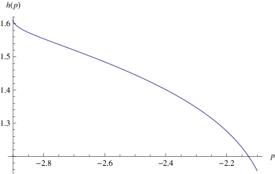
The numerical solutions for the flow are given in Fig.1 and Fig.2.
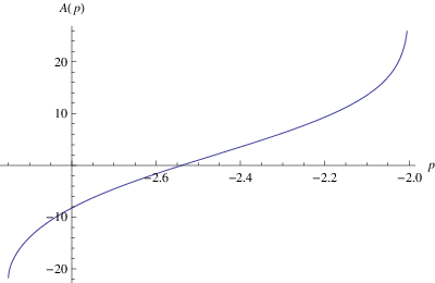
The gravitino variation gives an equation for A⁡(p)A(p), with t=2t=2,

d​Ad​p\displaystyle\frac{dA}{dp} =\displaystyle= −8​gp2​[(p2−2)​p2−4+p3−4​p]p2−4​(p​p2−4+p2−4)2×\displaystyle-\frac{8g_{p}^{2}[(p^{2}-2)\sqrt{p^{2}-4}+p^{3}-4p]}{\sqrt{p^{2}-4}(p\sqrt{p^{2}-4}+p^{2}-4)^{2}}\times (94)
[(p+6)h(p)2(2z1(p)+1)+ph(p)(1−2z1(p)(4z1(p)+3))\displaystyle[(p+6)h(p)^{2}(2z_{1}(p)+1)+ph(p)(1-2z_{1}(p)(4z_{1}(p)+3))
−2z1(p)(2pz1(p)+2p+3)−3]/[−4(2h(p)+1)z1(p)2\displaystyle-2z_{1}(p)(2pz_{1}(p)+2p+3)-3]/[-4(2h(p)+1)z_{1}(p)^{2}
+2((h(p)−3)h(p)−2)z1(p)+h(p)(h(p)+1)].\displaystyle+2((h(p)-3)h(p)-2)z_{1}(p)+h(p)(h(p)+1)].

Choosing g2​s=−1g_{2s}=-1 and gp=1g_{p}=1, we find the numerical solution for AA as shown in Fig.3.

Refer to caption
Figure 1: h⁡(p)h(p) solution.
Refer to caption
Figure 2: z1​(p)z_{1}(p) solution.
Refer to caption
Figure 3: A⁡(p)A(p) solution.

In this flow, the point IV is the UV fixed point, and V is the IR. The ratio of the central charges is

cU​VcI​R=(gn+gp)24​gn​gp.\frac{c_{UV}}{c_{IR}}=\frac{(g_{n}+g_{p})^{2}}{4g_{n}g_{p}}. (95)

This ratio is greater than 1 in consistent with the c-theorem. We also compute the scalar mass matrices at both critical points, but the form of the matrices is too complicated to be written here. We give only the numerical values of the eigenvalues in our choice of gp=1g_{p}=1, gn=2g_{n}=2 and g2​s=−1g_{2s}=-1.

  • •

    IV: Eigenvalues of M2​R2M^{2}R^{2} are (3.70,−1.00,−1.00,−0.97,0.36,0.36,0.00,0.00)(3.70,-1.00,-1.00,-0.97,0.36,0.36,0.00,0.00)
    with eigenvectors

    U1\displaystyle U_{1} =\displaystyle= (−0.47,−0.47,−0.44,−0.44,−0.16,−0.16,−0.24,−0.24)\displaystyle(-0.47,-0.47,-0.44,-0.44,-0.16,-0.16,-0.24,-0.24)
    U2\displaystyle U_{2} =\displaystyle= (0.33,−0.33,0.44,−0.44,0.00,0.00,0.44,−0.44)\displaystyle(0.33,-0.33,0.44,-0.44,0.00,0.00,0.44,-0.44)
    U3\displaystyle U_{3} =\displaystyle= (0.63,−0.63,−0.23,0.23,0.00,0.00,−0.23,0.23)\displaystyle(0.63,-0.63,-0.23,0.23,0.00,0.00,-0.23,0.23)
    U4\displaystyle U_{4} =\displaystyle= (0.47,0.47,−0.44,−0.44,0.16,0.16,−0.24,−0.24)\displaystyle(0.47,0.47,-0.44,-0.44,0.16,0.16,-0.24,-0.24)
    U5\displaystyle U_{5} =\displaystyle= (0.00,0.00,−0.49,0.49,−0.14,0.14,0.49,−0.49)\displaystyle(0.00,0.00,-0.49,0.49,-0.14,0.14,0.49,-0.49)
    U6\displaystyle U_{6} =\displaystyle= (0.00,0.00,−0.10,0.10,0.69,−0.69,0.10,−0.10)\displaystyle(0.00,0.00,-0.10,0.10,0.69,-0.69,0.10,-0.10)
    U7\displaystyle U_{7} =\displaystyle= (0.22,0.22,−0.06,−0.06,−0.66,−0.66,0.11,0.11)\displaystyle(0.22,0.22,-0.06,-0.06,-0.66,-0.66,0.11,0.11)
    U8\displaystyle U_{8} =\displaystyle= (−0.04,−0.04,−0.33,−0.33,0.12,0.12,0.61,0.61).\displaystyle(-0.04,-0.04,-0.33,-0.33,0.12,0.12,0.61,0.61). (96)

    Our flow ansatz corresponds to U4U_{4} with Δ=1.168\Delta=1.168 which is dual to a relevant operator. Note also that, our ansatz does not correspond to the one which saturates the bound M2​R2=−1M^{2}R^{2}=-1. This means the dual operator is not the most relevant one.

  • •

    V: Eigenvalues of M2​R2M^{2}R^{2} are (4.17,3.33,3.33,3.33,0.84,0.84,0.84,0.00)(4.17,3.33,3.33,3.33,0.84,0.84,0.84,0.00)
    with eigenvectors

    V1\displaystyle V_{1} =\displaystyle= (−0.211,−0.894,−0.211,−0.211,−0.130,−0.130,−0.130,−0.130)\displaystyle(-0.211,-0.894,-0.211,-0.211,-0.130,-0.130,-0.130,-0.130)
    V2\displaystyle V_{2} =\displaystyle= (0.201,−0.031,0.063,−0.159,−0.609,0.001,0.090,0.742)\displaystyle(0.201,-0.031,0.063,-0.159,-0.609,0.001,0.090,0.742)
    V3\displaystyle V_{3} =\displaystyle= (0.390,−0.398,0.523,0.432,0.400,0.011,−0.103,0.241)\displaystyle(0.390,-0.398,0.523,0.432,0.400,0.011,-0.103,0.241)
    V4\displaystyle V_{4} =\displaystyle= (−0.293,0.159,0.015,−0.258,0.359,−0.004,−0.801,0.227)\displaystyle(-0.293,0.159,0.015,-0.258,0.359,-0.004,-0.801,0.227)
    V5\displaystyle V_{5} =\displaystyle= (0.255,0.002,−0.712,0.572,−0.039,0.086,−0.300,0.046)\displaystyle(0.255,0.002,-0.712,0.572,-0.039,0.086,-0.300,0.046)
    V6\displaystyle V_{6} =\displaystyle= (−0.146,0.011,0.387,0.287,−0.526,0.391,−0.384,−0.411)\displaystyle(-0.146,0.011,0.387,0.287,-0.526,0.391,-0.384,-0.411)
    V7\displaystyle V_{7} =\displaystyle= (0.757,0.004,−0.047,−0.499,0.007,0.156,−0.207,−0.328)\displaystyle(0.757,0.004,-0.047,-0.499,0.007,0.156,-0.207,-0.328)
    V8\displaystyle V_{8} =\displaystyle= (0.130,0.130,0.130,0.130,−0.211,−0.893,−0.211,−0.211).\displaystyle(0.130,0.130,0.130,0.130,-0.211,-0.893,-0.211,-0.211). (97)

    Our flow ansatz corresponds to V1V_{1} with Δ=3.275\Delta=3.275 which is dual to an irrelevant operator.

The behavior near r→∞r\rightarrow\infty can be obtained as in the previous case. With gp=1g_{p}=1, gn=2g_{n}=2, and g2​s=−1g_{2s}=-1, we find that

p⁡(r)\displaystyle p(r) ∼\displaystyle\sim e−2r/R,z1(r),h(r)∼e−1.168r/R.\displaystyle e^{-2r/R},\qquad z_{1}(r),\phantom{a}h(r)\sim e^{-1.168r/R}. (98)

At the IR point, we find

z1​(r),h⁡(r),p⁡(r)∼e1.275​r/R.z_{1}(r),\phantom{a}h(r),\phantom{a}p(r)\sim e^{1.275r/R}. (99)

From the dominant term near the UV fixed point, we see that the flow solution describes the deformation of the UV theory by a vacuum expectation value of an operator of dimension 1.1681.168. We find that this flow is also a v.e.v. flow. The corresponding operator in the IR theory is an irrelevant operator of dimension 3.2753.275.

5 Vacua of the N=8N=8 Theory

In this section, we study a gauging of an N=8N=8 theory. We restrict our discussion to the target space S​O​(8,8)S​O​(8)×S​O​(8)\frac{SO(8,8)}{SO(8)\times SO(8)}. We parametrize the coset elements LL as in the N=4N=4 case, but now obviously ee is an element of G​L​(8,𝐑)GL(8,\bf R) and BB is an antisymmetric 8×88\times 8 matrix. The resulting LL depends on 92 parameters, but, again using the right action of a diagonal S​O​(8)SO(8), one can bring ee to an upper triangular form, thereby reducing the number of parameters to 64. As for the non compact generators, the Ya​bY^{ab} introduced before carry over in the obvious way to the present case, with a,b=1,…,8a,b=1,\dots,8.
We are going to gauge the subgroup (S​O​(4)⋉𝐑6)2(SO(4)\ltimes{\bf R}^{6})^{2}. Accordingly, we introduce gauge group generators:

t𝒜=(a10000a20000a10000a2),tℬ=(b10b100b20b2−b10−b100−b20−b2).t^{\mathcal{A}}=\left(\begin{array}[]{cccc}a_{1}&0&0&0\\ 0&a_{2}&0&0\\ 0&0&a_{1}&0\\ 0&0&0&a_{2}\\ \end{array}\right),\qquad t^{\mathcal{B}}=\left(\begin{array}[]{cccc}b_{1}&0&b_{1}&0\\ 0&b_{2}&0&b_{2}\\ -b_{1}&0&-b_{1}&0\\ 0&-b_{2}&0&-b_{2}\\ \end{array}\right). (100)

Here all entries are 4×44\times 4 matrices, a1a_{1} (a2)(a_{2}) are generators of the first (second) S​O​(4)SO(4), b1b_{1} and b2b_{2} are antisymmetric and correspond to independent shifts of BB. More precisely, the upper and lower 4×44\times 4 diagonal blocks of BB will be shifted by 2​b12b_{1} and 2​b22b_{2}, respectively, and therefore could be set to zero. Generators carrying index 1 commute with those carrying index 2, and one checks the structure of the gauge group stated above. The ff-tensors are constructed as follows: we choose a basis of symmetric, real S​O​(8)SO(8) γ\gamma-matrices with 8×88\times 8 off-diagonal blocks ΓI\Gamma^{I}, so that:

fa​b,c​dI​J=−12​Tr​(εb​a​[ΓI,ΓJ]​εc​d).f^{IJ}_{ab,cd}=-\frac{1}{2}\textrm{Tr}(\varepsilon^{ba}[\Gamma^{I},\Gamma^{J}]\varepsilon^{cd}). (101)

As for the embedding tensor Θ\Theta, the structure discussed in the N=4N=4 case extends naturally to the present case, and now we expect a priori 8 couplings corresponding to the 8 S​U​(2)SU(2)’s (including the ℬ\mathcal{B} generators). We then proceed first by computing the 𝒱\mathcal{V}’s which are given in the Appendix A and then the TT tensors which are given by:

TL​J,M​K\displaystyle T^{LJ,MK} =\displaystyle= g1​s​(𝒱+aL​J,P​Q​𝒱+bM​K,P​Q+𝒱+bL​J,P​Q​𝒱+aM​K,P​Q)+g1​a​(𝒱−aL​J,P​Q​𝒱−bM​K,P​QCLOSE\displaystyle g_{1s}(\mathcal{V}^{LJ,PQ}_{+\textrm{a}}\mathcal{V}^{MK,PQ}_{+\textrm{b}}+\mathcal{V}^{LJ,PQ}_{+\textrm{b}}\mathcal{V}^{MK,PQ}_{+\textrm{a}})+g_{1a}(\mathcal{V}^{LJ,PQ}_{-\textrm{a}}\mathcal{V}^{MK,PQ}_{-\textrm{b}}
OPEN+𝒱−bL​J,P​Q​𝒱−aM​K,P​Q)+g2​s​(𝒱+aL​J,P′​Q′​𝒱+bM​K,P′​Q′+𝒱+bL​J,P′​Q′​𝒱+aM​K,P′​Q′)\displaystyle+\mathcal{V}^{LJ,PQ}_{-\textrm{b}}\mathcal{V}^{MK,PQ}_{-\textrm{a}})+g_{2s}(\mathcal{V}^{LJ,P^{\prime}Q^{\prime}}_{+\textrm{a}}\mathcal{V}^{MK,P^{\prime}Q^{\prime}}_{+\textrm{b}}+\mathcal{V}^{LJ,P^{\prime}Q^{\prime}}_{+\textrm{b}}\mathcal{V}^{MK,P^{\prime}Q^{\prime}}_{+\textrm{a}})
+g2​a​(𝒱−aL​J,P′​Q′​𝒱−bM​K,P′​Q′+𝒱−bL​J,P′​Q′​𝒱−aM​K,P′​Q′)+h1​s​𝒱+bL​J,P​Q​𝒱+bM​K,P​Q\displaystyle+g_{2a}(\mathcal{V}^{LJ,P^{\prime}Q^{\prime}}_{-\textrm{a}}\mathcal{V}^{MK,P^{\prime}Q^{\prime}}_{-\textrm{b}}+\mathcal{V}^{LJ,P^{\prime}Q^{\prime}}_{-\textrm{b}}\mathcal{V}^{MK,P^{\prime}Q^{\prime}}_{-\textrm{a}})+h_{1s}\mathcal{V}_{+\textrm{b}}^{LJ,PQ}\mathcal{V}_{+\textrm{b}}^{MK,PQ}
+h1​a​𝒱−bL​J,P​Q​𝒱−bM​K,P​Q+h2​s​𝒱+bL​J,P′​Q′​𝒱+bM​K,P′​Q′+h2​a​𝒱−bL​J,P′​Q′​𝒱−bM​K,P′​Q′,\displaystyle+h_{1a}\mathcal{V}_{-\textrm{b}}^{LJ,PQ}\mathcal{V}_{-\textrm{b}}^{MK,PQ}+h_{2s}\mathcal{V}_{+\textrm{b}}^{LJ,P^{\prime}Q^{\prime}}\mathcal{V}_{+\textrm{b}}^{MK,P^{\prime}Q^{\prime}}+h_{2a}\mathcal{V}_{-\textrm{b}}^{LJ,P^{\prime}Q^{\prime}}\mathcal{V}_{-\textrm{b}}^{MK,P^{\prime}Q^{\prime}},
Ta​bL​J\displaystyle T^{LJ}_{ab} =\displaystyle= g1​s​(𝒱+aL​J,P​Q​𝒱+ba​bP​Q+𝒱+bL​J,P​Q​𝒱+aa​bP​Q)+g1​a​(𝒱−aL​J,P​Q​𝒱−ba​bP​QCLOSE\displaystyle g_{1s}(\mathcal{V}_{+\textrm{a}}^{LJ,PQ}{\mathcal{V}_{+\textrm{b}}}^{PQ}_{ab}+\mathcal{V}_{+\textrm{b}}^{LJ,PQ}{\mathcal{V}_{+\textrm{a}}}^{PQ}_{ab})+g_{1a}(\mathcal{V}_{-\textrm{a}}^{LJ,PQ}{\mathcal{V}_{-\textrm{b}}}^{PQ}_{ab} (102)
OPEN+𝒱−bL​J,P​Q​𝒱−aa​bP​Q)+g2​s​(𝒱+aL​J,P′​Q′​𝒱+ba​bP′​Q′+𝒱+bL​J,P′​Q′​𝒱+aa​bP′​Q′)\displaystyle+\mathcal{V}_{-\textrm{b}}^{LJ,PQ}{\mathcal{V}_{-\textrm{a}}}^{PQ}_{ab})+g_{2s}(\mathcal{V}_{+\textrm{a}}^{LJ,P^{\prime}Q^{\prime}}{\mathcal{V}_{+\textrm{b}}}^{P^{\prime}Q^{\prime}}_{ab}+\mathcal{V}_{+\textrm{b}}^{LJ,P^{\prime}Q^{\prime}}{\mathcal{V}_{+\textrm{a}}}^{P^{\prime}Q^{\prime}}_{ab})
+g2​a​(𝒱−aL​J,P′​Q′​𝒱−ba​bP′​Q′+𝒱−bL​J,P′​Q′​𝒱−aa​bP′​Q′)+h1​s​𝒱+bL​J,P​Q​𝒱+ba​bP​Q\displaystyle+g_{2a}(\mathcal{V}_{-\textrm{a}}^{LJ,P^{\prime}Q^{\prime}}{\mathcal{V}_{-\textrm{b}}}^{P^{\prime}Q^{\prime}}_{ab}+\mathcal{V}_{-\textrm{b}}^{LJ,P^{\prime}Q^{\prime}}{\mathcal{V}_{-\textrm{a}}}^{P^{\prime}Q^{\prime}}_{ab})+h_{1s}\mathcal{V}^{LJ,PQ}_{+\textrm{b}}{\mathcal{V}_{+\textrm{b}}}^{PQ}_{ab}
+h1​a​𝒱−bL​J,P​Q​𝒱−ba​bP​Q+h2​s​𝒱+bL​J,P′​Q′​𝒱+ba​bP′​Q′+h2​a​𝒱−bL​J,P′​Q′​𝒱−ba​bP′​Q′,\displaystyle+h_{1a}\mathcal{V}^{LJ,PQ}_{-\textrm{b}}{\mathcal{V}_{-\textrm{b}}}^{PQ}_{ab}+h_{2s}\mathcal{V}^{LJ,P^{\prime}Q^{\prime}}_{+\textrm{b}}{\mathcal{V}_{+\textrm{b}}}^{P^{\prime}Q^{\prime}}_{ab}+h_{2a}\mathcal{V}^{LJ,P^{\prime}Q^{\prime}}_{-\textrm{b}}{\mathcal{V}_{-\textrm{b}}}^{P^{\prime}Q^{\prime}}_{ab},

where P,Q,…=1,…,4P,Q,\ldots=1,\ldots,4 and P′,Q′,…=5,…,8P^{\prime},Q^{\prime},\ldots=5,\ldots,8. Here L,J,M,KL,J,M,K are S​O​(8)SO(8) R-symmetry indices, and a,b=1,…,8a,b=1,\dots,8 label the 64 non-compact generators in S​O​(8,8)SO(8,8). P,Q=1,…,4P,Q=1,\dots,4 and P′,Q′=5,…,8P^{\prime},Q^{\prime}=5,\dots,8 label the first and second S​O​(4)SO(4), respectively. We have included also the 8 coupling constants, but actually, consistency imposes relations among them:

g1​a\displaystyle g_{1a} =\displaystyle= −g1​s,g2​a=−g2​s\displaystyle-g_{1s},\qquad g_{2a}=-g_{2s}
h1​a\displaystyle h_{1a} =\displaystyle= −h1​s,andh2​a=−h2​s.\displaystyle-h_{1s},\qquad\textrm{and}\qquad h_{2a}=-h_{2s}. (103)

Notice that if we set the type-2 couplings to zero i.e. g2​s=g2​a=h2​s=h2​a=0g_{2s}=g_{2a}=h_{2s}=h_{2a}=0, we decouple the second S​O​(4)SO(4) and therefore we recover a truncation of the single S​O​(4)SO(4) gauging studied in [9] as the supergravity dual of the D1-D5 system in IIB theory on K​3K3 or T4T^{4}. It can be obtained by reducing (2,0) six-dimensional supergravity on A​d​S3×S3AdS_{3}\times S^{3}.
A simple class of supersymmetric A​d​SAdS vacua can be obtained as follows. We parameterize ee and BB as:

e=(a1000e15e16e17e180a200e25e26e27e2800a30e35e36e37e38000a4e45e46e47e480000a500000000a600000000a700000000a8)e=\left(\begin{array}[]{cccccccc}a_{1}&0&0&0&e_{15}&e_{16}&e_{17}&e_{18}\\ 0&a_{2}&0&0&e_{25}&e_{26}&e_{27}&e_{28}\\ 0&0&a_{3}&0&e_{35}&e_{36}&e_{37}&e_{38}\\ 0&0&0&a_{4}&e_{45}&e_{46}&e_{47}&e_{48}\\ 0&0&0&0&a_{5}&0&0&0\\ 0&0&0&0&0&a_{6}&0&0\\ 0&0&0&0&0&0&a_{7}&0\\ 0&0&0&0&0&0&0&a_{8}\\ \end{array}\right) (104)
B=(0000b15b16b17b180000b25b26b27b280000b35b36b37b380000b45b46b47b48−b15−b25−b35−b450000−b16−b26−b36−b460000−b17−b27−b37−b470000−b18−b28−b38−b480000).B=\left(\begin{array}[]{cccccccc}0&0&0&0&b_{15}&b_{16}&b_{17}&b_{18}\\ 0&0&0&0&b_{25}&b_{26}&b_{27}&b_{28}\\ 0&0&0&0&b_{35}&b_{36}&b_{37}&b_{38}\\ 0&0&0&0&b_{45}&b_{46}&b_{47}&b_{48}\\ -b_{15}&-b_{25}&-b_{35}&-b_{45}&0&0&0&0\\ -b_{16}&-b_{26}&-b_{36}&-b_{46}&0&0&0&0\\ -b_{17}&-b_{27}&-b_{37}&-b_{47}&0&0&0&0\\ -b_{18}&-b_{28}&-b_{38}&-b_{48}&0&0&0&0\\ \end{array}\right). (105)

We have used the shift symmetry to set to zero the diagonal 4×44\times 4 blocks of BB and the S​O​(4)×S​O​(4)SO(4)\times SO(4) left action to diagonalize the diagonal blocks of ee. For diagonal e=(a1,a2,a3,a4,a5,a6,a7,a8)e=(a_{1},a_{2},a_{3},a_{4},a_{5},a_{6},a_{7},a_{8}) and B=0B=0, we cannot find any interesting solutions apart from the trivial one with (4,4) supersymmetry. All the truncations below have been checked to be consistent, in the sense that there are no tadpoles for the remaining scalars.
We find a class of solutions by setting:

a2\displaystyle a_{2} =\displaystyle= a3=a4=a1\displaystyle a_{3}=a_{4}=a_{1}
a6\displaystyle a_{6} =\displaystyle= a7=a8=a5\displaystyle a_{7}=a_{8}=a_{5}
b15\displaystyle b_{15} =\displaystyle= 14​(c15−c26−c37+c48)b16=14​(−c16−c25−c38−c47)\displaystyle\frac{1}{4}(c_{15}-c_{26}-c_{37}+c_{48})\qquad b_{16}=\frac{1}{4}(-c_{16}-c_{25}-c_{38}-c_{47})
b17\displaystyle b_{17} =\displaystyle= 14​(c18+c27−c36−c45)b18=14​(c17−c28+c35−c46)\displaystyle\frac{1}{4}(c_{18}+c_{27}-c_{36}-c_{45})\qquad b_{18}=\frac{1}{4}(c_{17}-c_{28}+c_{35}-c_{46})
b25\displaystyle b_{25} =\displaystyle= 14​(−c16−c25+c38+c47)b26=14​(−c15+c26−c37+c48)\displaystyle\frac{1}{4}(-c_{16}-c_{25}+c_{38}+c_{47})\qquad b_{26}=\frac{1}{4}(-c_{15}+c_{26}-c_{37}+c_{48})
b27\displaystyle b_{27} =\displaystyle= 14​(c17−c28−c35+c46)b28=14​(−c18−c27−c36−c45)\displaystyle\frac{1}{4}(c_{17}-c_{28}-c_{35}+c_{46})\qquad b_{28}=\frac{1}{4}(-c_{18}-c_{27}-c_{36}-c_{45})
b35\displaystyle b_{35} =\displaystyle= 14​(c18−c27+c36−c45)b36=14​(−c17−c28+c35+c46)\displaystyle\frac{1}{4}(c_{18}-c_{27}+c_{36}-c_{45})\qquad b_{36}=\frac{1}{4}(-c_{17}-c_{28}+c_{35}+c_{46})
b37\displaystyle b_{37} =\displaystyle= 14​(−c15−c26−c37−c48)b38=14​(−c16+c25+c38−c47)\displaystyle\frac{1}{4}(-c_{15}-c_{26}-c_{37}-c_{48})\qquad b_{38}=\frac{1}{4}(-c_{16}+c_{25}+c_{38}-c_{47})
b45\displaystyle b_{45} =\displaystyle= 14​(−c17−c28−c35−c46)b46=14​(−c18+c27+c36−c45)\displaystyle\frac{1}{4}(-c_{17}-c_{28}-c_{35}-c_{46})\qquad b_{46}=\frac{1}{4}(-c_{18}+c_{27}+c_{36}-c_{45})
b47\displaystyle b_{47} =\displaystyle= 14​(−c16+c25−c38+c47)b48=14​(c15+c26−c37−c48),\displaystyle\frac{1}{4}(-c_{16}+c_{25}-c_{38}+c_{47})\qquad b_{48}=\frac{1}{4}(c_{15}+c_{26}-c_{37}-c_{48}), (106)

and all other parameters are zero. We can choose

c16\displaystyle c_{16} =\displaystyle= c17=c18=c25=c27=c28=0\displaystyle c_{17}=c_{18}=c_{25}=c_{27}=c_{28}=0
c35\displaystyle c_{35} =\displaystyle= c36=c38=c45=c46=c47=0.\displaystyle c_{36}=c_{38}=c_{45}=c_{46}=c_{47}=0. (107)

Supersymmetric vacua require

g1​s=−a12​h1​sg2​s=−a52​h2​sh2​s=a14a54​h1​s.g_{1s}=-a_{1}^{2}h_{1s}\qquad g_{2s}=-a_{5}^{2}h_{2s}\qquad h_{2s}=\frac{a_{1}^{4}}{a_{5}^{4}}h_{1s}. (108)
  • •

    (1,1) critical point
    This point is given by c15=0c_{15}=0,

    A1\displaystyle A_{1} =\displaystyle= (−16​g1​s2h1​s,16​g1​s2h1​s,−8​g1​s2h1​s​4+a12​a52​c262,8​g1​s2h1​s​4+a12​a52​c262CLOSE,\displaystyle(-\frac{16g_{1s}^{2}}{h_{1s}},\frac{16g_{1s}^{2}}{h_{1s}},-\frac{8g_{1s}^{2}}{h_{1s}}\sqrt{4+a_{1}^{2}a_{5}^{2}c_{26}^{2}},\frac{8g_{1s}^{2}}{h_{1s}}\sqrt{4+a_{1}^{2}a_{5}^{2}c_{26}^{2}}, (109)
    −8​g1​s2h1​s​4+a12​a52​c372,8​g1​s2h1​s​4+a12​a52​c372,−8​g1​s2h1​s​4+a12​a52​c482,\displaystyle-\frac{8g_{1s}^{2}}{h_{1s}}\sqrt{4+a_{1}^{2}a_{5}^{2}c_{37}^{2}},\frac{8g_{1s}^{2}}{h_{1s}}\sqrt{4+a_{1}^{2}a_{5}^{2}c_{37}^{2}},-\frac{8g_{1s}^{2}}{h_{1s}}\sqrt{4+a_{1}^{2}a_{5}^{2}c_{48}^{2}},
    OPEN8​g1​s2h1​s​4+a12​a52​c482)\displaystyle\frac{8g_{1s}^{2}}{h_{1s}}\sqrt{4+a_{1}^{2}a_{5}^{2}c_{48}^{2}})

    and V0=−1024​g1​s4h1​s2V_{0}=-\frac{1024g_{1s}^{4}}{h_{1s}^{2}}.

  • •

    (2,2) critical point
    This point is given by c15=0c_{15}=0 and c26=0c_{26}=0.

  • •

    (3,3) critical point
    This point is given by c15=0c_{15}=0,c26=0c_{26}=0 and c37=0c_{37}=0.

  • •

    (4,4) critical point
    This point is given by c15=0c_{15}=0, c26=0c_{26}=0, c37=0c_{37}=0 and c48=0c_{48}=0.

All of them have the same cosmological constant. A1A_{1} for the last three points is given by setting some of the appropriate values of cc’s to zero in (109).
We also find other solutions with non zero parameters

a2=a3=a4=a1a6=a7=a8=a5\displaystyle a_{2}=a_{3}=a_{4}=a_{1}\qquad a_{6}=a_{7}=a_{8}=a_{5}
e15=e26=e37=e48=e\displaystyle e_{15}=e_{26}=e_{37}=e_{48}=e
b16=−b25b38=−b47\displaystyle b_{16}=-b_{25}\qquad b_{38}=-b_{47} (110)

subject to these relations a52+e2=−g2​sh2​sa_{5}^{2}+e^{2}=-\frac{g_{2s}}{h_{2s}}, a12=−g1​sh1​sa_{1}^{2}=-\frac{g_{1s}}{h_{1s}} and g1​s2h1​s=g2​s2h2​s\frac{g_{1s}^{2}}{h_{1s}}=\frac{g_{2s}^{2}}{h_{2s}}. Note that in this case, we also turn on some off-diagonal elements of ee. The solutions are given by:

  • •

    (2,2) critical point
    This solution has A1=16​g1​s2h1​sA_{1}=\frac{16g_{1s}^{2}}{h_{1s}} giving the same cosmological constant as in the previous case.

  • •

    (3,2) critical point
    This can be obtained from the previous case by setting b25=b47b_{25}=b_{47} or b25=−b47b_{25}=-b_{47}.

So, there is no possible flow solution between all these critical points.

6 Conclusions

In this paper, we have studied three dimensional gauged supergravities and their A​d​S3AdS_{3} supersymmetric vacua. We have discussed the N=4N=4 and N=8N=8 theories with S​O​(4)⋉𝐑𝟔SO(4)\ltimes\bf{R}^{6} and (S​O​(4)⋉𝐑𝟔)𝟐(SO(4)\ltimes\bf{R}^{6})^{2} gaugings, respectively. Several supersymmetric A​d​S3AdS_{3} vacua with different amount of supersymmetry have been found.
In the N=4N=4 theory, we have found analytic solutions interpolating between two (3,1) vacua. These solutions describe Renormalization Group flows between two fixed points of the dual boundary field theory. We have checked that the flows agree with the c-theorem, in particular the central charges of UV fixed points are strictly greater than those of the IR ones. We have also found a numerical solution describing the flow between (2,0) vacua with similar qualitative features. In both cases, we found v.e.v. flows, i.e. flows driven by vacuum expectation values of relevant operators with dimensions Δ=1\Delta=1 and Δ=1.168\Delta=1.168, respectively, as opposed to the most common case where the flow is driven by a perturbing relevant operator.
In the N=8N=8 theory, we have found several vacua. However, they all have the same cosmological constant/central charge and the flow issue does not arise.
The gaugings considered here are of non semi-simple Chern-Simons type, giving rise to semi-simple Yang-Mills theories. In the N=8N=8 case, the (4,4)(4,4) point is related to the KK reduction of type IIB theory on A​d​S3×S3×S3×S1AdS_{3}\times S^{3}\times S^{3}\times S^{1}, and it would be interesting to identify the marginal deformations which take the theory to other less supersymmetric vacua, i.e. to generalize the discussion of [16], where the marginal deformation from (4,4)(4,4) to (3,3)(3,3) vacua has been worked out in detail, to the (k,k)(k,k) vacua with k<3k<3. The N=4N=4 case seems to be related, via a ℤ2\mathbb{Z}_{2} projection, to the N=8N=8 theory, and it would be interesting to see how this is acting on the corresponding type IIB theory background. This would presumably help us in understanding the nature of the dual S​C​F​T2SCFT_{2}.

Acknowledgments.
This work has been supported in part by the EU grant UNILHC-Grant Agreement PITN-GA-2009-237920.

Appendix A Essential formulae

In this appendix, we give the expressions for the 𝒱\mathcal{V}’s. Indices referring to each target space coordinates, i,j,k,…i,j,k,\ldots, will be traded by a pair of indices of the type a,b,c,…a,b,c,\ldots from 1 to 4. Antisymmetric pairs of capital letters I,J,K,…I,J,K,\ldots label S​O​(4)SO(4) adjoint indices.

𝒱±aL​J,M​K\displaystyle\mathcal{V}_{\pm\textrm{a}}^{LJ,MK} =\displaystyle= −14​Tr​[(e1t​J+L​J​X1t+X1​J+L​J​e1)​J±M​K+(e2t​J−L​J​X2t+X2​J−L​J​e2)​J±M​K],\displaystyle-\frac{1}{4}\textrm{Tr}[(e_{1}^{t}J_{+}^{LJ}X_{1}^{t}+X_{1}J_{+}^{LJ}e_{1})J_{\pm}^{MK}+(e_{2}^{t}J_{-}^{LJ}X_{2}^{t}+X_{2}J_{-}^{LJ}e_{2})J_{\pm}^{MK}],
𝒱±1,2​aa​bM​K\displaystyle{\mathcal{V}_{\pm 1,2\textrm{a}}}^{MK}_{ab} =\displaystyle= Tr​[(e1,2t​εa​b​X1,2t+Y1,2​εa​b​e1,2)​J±M​K],\displaystyle\textrm{Tr}[(e_{1,2}^{t}\varepsilon_{ab}X_{1,2}^{t}+Y_{1,2}\varepsilon_{ab}e_{1,2})J_{\pm}^{MK}],
𝒱±bL​J,M​K\displaystyle\mathcal{V}_{\pm\textrm{b}}^{LJ,MK} =\displaystyle= −14​Tr​[(e1t​J+L​J​e1t+e2t​J−L​J​e2t)​J±M​K],\displaystyle-\frac{1}{4}\textrm{Tr}[(e_{1}^{t}J_{+}^{LJ}e_{1}^{t}+e_{2}^{t}J_{-}^{LJ}e_{2}^{t})J_{\pm}^{MK}],
𝒱±1,2​ba​bM​K\displaystyle{\mathcal{V}_{\pm 1,2\textrm{b}}}^{MK}_{ab} =\displaystyle= Tr​(e1,2t​εa​b​e1,2​J±M​K).\displaystyle\textrm{Tr}(e_{1,2}^{t}\varepsilon_{ab}e_{1,2}J_{\pm}^{MK}). (111)

The string of indices ±1,2​a\pm 1,2\textrm{a} (±1,2​b\pm 1,2\textrm{b}) indicates 𝒜\mathcal{A} (ℬ\mathcal{B})-type gauging in the first (second) space with (anti-)self-dual S​U​(2)SU(2).
For completeness, we give below the analogous expressions for the N=8N=8 case:

𝒱±aL​J,M​K\displaystyle{\mathcal{V}_{{\pm\textrm{a}}}}^{LJ,MK} =\displaystyle= 14​2​Tr​[ΓJ​L​(e​J±M​K​X+Xt​J±M​K​et)],\displaystyle\frac{1}{4\sqrt{2}}\textrm{Tr}[\Gamma^{JL}(eJ_{\pm}^{MK}X+X^{t}J_{\pm}^{MK}e^{t})],
𝒱±bL​J,M​K\displaystyle{\mathcal{V}_{\pm\textrm{b}}}^{LJ,MK} =\displaystyle= 12​2​Tr​[J±J​L​e​ΓM​K​et],\displaystyle\frac{1}{2\sqrt{2}}\textrm{Tr}[J_{\pm}^{JL}e\Gamma^{MK}e^{t}],
𝒱±aa​bM​K\displaystyle{\mathcal{V}_{\pm\textrm{a}}}^{MK}_{ab} =\displaystyle= 12​Tr​[εa​b​(Xt​J±M​K​et+e​J±M​K​Y)],\displaystyle\frac{1}{\sqrt{2}}\textrm{Tr}[\varepsilon_{ab}(X^{t}J_{\pm}^{MK}e^{t}+eJ_{\pm}^{MK}Y)],
𝒱± bM​Ka​b\displaystyle{\mathcal{V}_{\pm\textrm{ b}}}^{MK}_{ab} =\displaystyle= 22​Tr​[εa​b​e​J±M​K​et].\displaystyle\frac{2}{\sqrt{2}}\textrm{Tr}[\varepsilon_{ab}eJ_{\pm}^{MK}e^{t}]. (112)

Here ΓJ​L=−[ΓJ,ΓL]/2\Gamma^{JL}=-[\Gamma^{J},\Gamma^{L}]/2 and all indices run from 1 to 8 and J±M​KJ_{\pm}^{MK} are the (anti-)self-dual S​U​(2)SU(2) generators in S​O​(4)×S​O​(4)⊂S​O​(8)SO(4)\times SO(4)\subset SO(8), corresponding to the first (second) S​O​(4)SO(4) for M,K=1,…,4M,K=1,\dots,4 (M,K=5,…,8M,K=5,\dots,8), respectively.

Appendix B The other vacua of the N=4N=4 theory

In this appendix, we give all vacua we have found in N=4N=4 theory apart from those involved in the flows.

B.1 (4,0) vacuum

  • •

    VI.

    e1\displaystyle e_{1} =\displaystyle= −2​(gn+gp)g2​s​𝕀4×4,e2=2​(gp−gn)g2​s​𝕀4×4,\displaystyle\sqrt{\frac{-2(g_{n}+g_{p})}{g_{2s}}}\mathbb{I}_{4\times 4},\qquad e_{2}=\sqrt{\frac{2(g_{p}-g_{n})}{g_{2s}}}\mathbb{I}_{4\times 4},
    A1\displaystyle A_{1} =\displaystyle= 32​gn​gpg2​s,andV0=−4096​gn2​gp2g2​s2.\displaystyle\frac{32g_{n}g_{p}}{g_{2s}},\qquad\textrm{and}\qquad V_{0}=-\frac{4096g_{n}^{2}g_{p}^{2}}{g_{2s}^{2}}. (113)

B.2 (3,0) vacua

  • •

    VII.

    e1\displaystyle e_{1} =\displaystyle= a⁡(1,−gm+gpgn+gp+g2​s​a2,1,1),e2=(gp2−gn2)gp2−gn2+g2​s​gp​a​a​𝕀4×4,\displaystyle a\Big(1,-\frac{g_{m}+g_{p}}{g_{n}+g_{p}+g_{2s}a^{2}},1,1\Big),\qquad e_{2}=\sqrt{\frac{(g_{p}^{2}-g_{n}^{2})}{g_{p}^{2}-g_{n}^{2}+g_{2s}g_{p}a}}a\mathbb{I}_{4\times 4},
    a\displaystyle a =\displaystyle= gn3−gn2​gp−gn​gp2+gp3+gn6−gn4​gp2−gn2​gp4+gp6gn​gp​g2​s\displaystyle\sqrt{\frac{g_{n}^{3}-g_{n}^{2}g_{p}-g_{n}g_{p}^{2}+g_{p}^{3}+\sqrt{g_{n}^{6}-g_{n}^{4}g_{p}^{2}-g_{n}^{2}g_{p}^{4}+g_{p}^{6}}}{g_{n}g_{p}g_{2s}}}
    A1\displaystyle A_{1} =\displaystyle= −8​(gn2−gp2)2g2​s​gn​gp,andV0=−256​(gn2−gp2)4(g2​s2​gn​gp)2\displaystyle-\frac{8(g_{n}^{2}-g_{p}^{2})^{2}}{g_{2s}g_{n}g_{p}},\qquad\textrm{and}\qquad V_{0}=\frac{-256(g_{n}^{2}-g_{p}^{2})^{4}}{(g_{2s}^{2}g_{n}g_{p})^{2}} (114)
  • •

    VIII.

    e1\displaystyle e_{1} =\displaystyle= a⁡(1,−gm+gpgn+gp+g2​s​a2,1,1),e2=(gp2−gn2)gp2−gn2+g2​s​gp​a​a​𝕀4×4,\displaystyle a\Big(1,-\frac{g_{m}+g_{p}}{g_{n}+g_{p}+g_{2s}a^{2}},1,1\Big),\qquad e_{2}=\sqrt{\frac{(g_{p}^{2}-g_{n}^{2})}{g_{p}^{2}-g_{n}^{2}+g_{2s}g_{p}a}}a\mathbb{I}_{4\times 4},
    a\displaystyle a =\displaystyle= gn3−gn2​gp−gn​gp2+gp3−gn6−gn4​gp2−gn2​gp4+gp6gn​gp​g2​s\displaystyle\sqrt{\frac{g_{n}^{3}-g_{n}^{2}g_{p}-g_{n}g_{p}^{2}+g_{p}^{3}-\sqrt{g_{n}^{6}-g_{n}^{4}g_{p}^{2}-g_{n}^{2}g_{p}^{4}+g_{p}^{6}}}{g_{n}g_{p}g_{2s}}}
    A1\displaystyle A_{1} =\displaystyle= −8​(gn2−gp2)2g2​s​gn​gp,andV0=−256​(gn2−gp2)4(g2​s2​gn​gp)2\displaystyle-\frac{8(g_{n}^{2}-g_{p}^{2})^{2}}{g_{2s}g_{n}g_{p}},\qquad\textrm{and}\qquad V_{0}=\frac{-256(g_{n}^{2}-g_{p}^{2})^{4}}{(g_{2s}^{2}g_{n}g_{p})^{2}} (115)

B.3 (2,0) vacua

  • •

    IX.

    e1=−(a1,a1,b1,b2)e2=(b1,b1,b2,b2)e_{1}=-(a_{1},a_{1},b_{1},b_{2})\qquad e_{2}=(b_{1},b_{1},b_{2},b_{2}) (116)
    a1\displaystyle a_{1} =\displaystyle= 2​gn2−gp2g2​s​(gn−gp+5​gn2+2​gn​gp+gp2)\displaystyle 2\sqrt{\frac{g_{n}^{2}-g_{p}^{2}}{g_{2s}(g_{n}-g_{p}+\sqrt{5g_{n}^{2}+2g_{n}g_{p}+g_{p}^{2}})}}
    a2\displaystyle a_{2} =\displaystyle= 2​gn2−gp2g2​s​(gp−gn+5​gp2+2​gn​gp+gn2)\displaystyle 2\sqrt{\frac{g_{n}^{2}-g_{p}^{2}}{g_{2s}(g_{p}-g_{n}+\sqrt{5g_{p}^{2}+2g_{n}g_{p}+g_{n}^{2}})}}
    b1\displaystyle b_{1} =\displaystyle= 2​gp2−gn2g2​s​(3​gn+gp−5​gn2+2​gp​gn+gp2)\displaystyle 2\sqrt{\frac{g_{p}^{2}-g_{n}^{2}}{g_{2s}(3g_{n}+g_{p}-\sqrt{5g_{n}^{2}+2g_{p}g_{n}+g_{p}^{2}})}}
    b2\displaystyle b_{2} =\displaystyle= 2​gn2−gp2g2​s​(gn2+2​gn​gp+5​gp2−gn−3​gp)\displaystyle 2\sqrt{\frac{g_{n}^{2}-g_{p}^{2}}{g_{2s}(\sqrt{g_{n}^{2}+2g_{n}g_{p}+5g_{p}^{2}}-g_{n}-3g_{p})}} (117)
    A1\displaystyle A_{1} =\displaystyle= −32​(gn−gp)2g2​sandV0=−4096​(gn−gp)4g2​s2.\displaystyle\frac{-32(g_{n}-g_{p})^{2}}{g_{2s}}\qquad\textrm{and}\qquad V_{0}=-\frac{4096(g_{n}-g_{p})^{4}}{g_{2s}^{2}}. (118)
  • •

    X.

    e1=(−a1,a1,a2,a2)e2=(b1,b1,b2,b2)e_{1}=(-a_{1},a_{1},a_{2},a_{2})\qquad e_{2}=(b_{1},b_{1},b_{2},b_{2}) (119)
    a1\displaystyle a_{1} =\displaystyle= 2​gp2−gn2g2​s​(gp−gn+5​gn2+2​gp​gn+gp2)\displaystyle 2\sqrt{\frac{g_{p}^{2}-g_{n}^{2}}{g_{2s}(g_{p}-g_{n}+\sqrt{5g_{n}^{2}+2g_{p}g_{n}+g_{p}^{2}})}}
    a2\displaystyle a_{2} =\displaystyle= 2​gp2−gn2g2​s​(gn−gp−5​gp2+2​gp​gn+gn2)\displaystyle 2\sqrt{\frac{g_{p}^{2}-g_{n}^{2}}{g_{2s}(g_{n}-g_{p}-\sqrt{5g_{p}^{2}+2g_{p}g_{n}+g_{n}^{2}})}}
    b1\displaystyle b_{1} =\displaystyle= 2​gp2−gn2g2​s​(3​gn+gp+5​gn2+2​gp​gn+gp2)\displaystyle 2\sqrt{\frac{g_{p}^{2}-g_{n}^{2}}{g_{2s}(3g_{n}+g_{p}+\sqrt{5g_{n}^{2}+2g_{p}g_{n}+g_{p}^{2}})}}
    b2\displaystyle b_{2} =\displaystyle= 2​gn2−gp2g2​s​(gn2+2​gn​gp+5​gp2−gn−3​gp)\displaystyle 2\sqrt{\frac{g_{n}^{2}-g_{p}^{2}}{g_{2s}(\sqrt{g_{n}^{2}+2g_{n}g_{p}+5g_{p}^{2}}-g_{n}-3g_{p})}} (120)
    A1\displaystyle A_{1} =\displaystyle= −32​(gn−gp)2g2​sandV0=−4096​(gn−gp)4g2​s2.\displaystyle\frac{-32(g_{n}-g_{p})^{2}}{g_{2s}}\qquad\textrm{and}\qquad V_{0}=-\frac{4096(g_{n}-g_{p})^{4}}{g_{2s}^{2}}. (121)
  • •

    XI.

    e1=(−a1,a1,a2,a2)e2=(b1,b1,b2,b2)e_{1}=(-a_{1},a_{1},a_{2},a_{2})\qquad e_{2}=(b_{1},b_{1},b_{2},b_{2}) (122)
    a1\displaystyle a_{1} =\displaystyle= 2​gp2−gn2g2​s​(gp−gn−5​gn2+2​gp​gn+gp2)\displaystyle 2\sqrt{\frac{g_{p}^{2}-g_{n}^{2}}{g_{2s}(g_{p}-g_{n}-\sqrt{5g_{n}^{2}+2g_{p}g_{n}+g_{p}^{2}})}}
    a2\displaystyle a_{2} =\displaystyle= 2​gp2−gn2g2​s​(gn−gp+5​gp2+2​gp​gn+gn2)\displaystyle 2\sqrt{\frac{g_{p}^{2}-g_{n}^{2}}{g_{2s}(g_{n}-g_{p}+\sqrt{5g_{p}^{2}+2g_{p}g_{n}+g_{n}^{2}})}}
    b1\displaystyle b_{1} =\displaystyle= 2​gp2−gn2g2​s​(3​gn+gp−5​gn2+2​gp​gn+gp2)\displaystyle 2\sqrt{\frac{g_{p}^{2}-g_{n}^{2}}{g_{2s}(3g_{n}+g_{p}-\sqrt{5g_{n}^{2}+2g_{p}g_{n}+g_{p}^{2}})}}
    b2\displaystyle b_{2} =\displaystyle= 2​gp2−gn2g2​s​(gn2+2​gn​gp+5​gp2+gn+3​gp)\displaystyle 2\sqrt{\frac{g_{p}^{2}-g_{n}^{2}}{g_{2s}(\sqrt{g_{n}^{2}+2g_{n}g_{p}+5g_{p}^{2}}+g_{n}+3g_{p})}} (123)
    A1\displaystyle A_{1} =\displaystyle= −32​(gn−gp)2g2​sandV0=−4096​(gn−gp)4g2​s2.\displaystyle\frac{-32(g_{n}-g_{p})^{2}}{g_{2s}}\qquad\textrm{and}\qquad V_{0}=-\frac{4096(g_{n}-g_{p})^{4}}{g_{2s}^{2}}. (124)
  • •

    XII.

    e1=(−a1,a1,a2,a2)e2=(b1,b1,b2,b2)e_{1}=(-a_{1},a_{1},a_{2},a_{2})\qquad e_{2}=(b_{1},b_{1},b_{2},b_{2}) (125)
    a1\displaystyle a_{1} =\displaystyle= gp−gng2​s​gn−gp+5​gn2+2​gn​gp+gp2gn\displaystyle\sqrt{\frac{g_{p}-g_{n}}{g_{2s}}}\sqrt{\frac{g_{n}-g_{p}+\sqrt{5g_{n}^{2}+2g_{n}g_{p}+g_{p}^{2}}}{g_{n}}}
    a2\displaystyle a_{2} =\displaystyle= gp−gng2​s​−gn−gp+gn2+2​gn​gp+5​gp2gp\displaystyle\sqrt{\frac{g_{p}-g_{n}}{g_{2s}}}\sqrt{-\frac{g_{n}-g_{p}+\sqrt{g_{n}^{2}+2g_{n}g_{p}+5g_{p}^{2}}}{g_{p}}}
    b1\displaystyle b_{1} =\displaystyle= gp−gng2​s​3​gn+gp−5​gn2+2​gn​gp+gp2gn\displaystyle\sqrt{\frac{g_{p}-g_{n}}{g_{2s}}}\sqrt{\frac{3g_{n}+g_{p}-\sqrt{5g_{n}^{2}+2g_{n}g_{p}+g_{p}^{2}}}{g_{n}}}
    b2\displaystyle b_{2} =\displaystyle= gp2−gn2g2​s​gp​−gn−gp+gn2+2​gn​gp+5​gp22​gp−gn2+2​gn​gp+5​gp2\displaystyle\sqrt{\frac{g_{p}^{2}-g_{n}^{2}}{g_{2s}g_{p}}}\sqrt{-\frac{g_{n}-g_{p}+\sqrt{g_{n}^{2}+2g_{n}g_{p}+5g_{p}^{2}}}{2g_{p}-\sqrt{g_{n}^{2}+2g_{n}g_{p}+5g_{p}^{2}}}} (126)
    A1\displaystyle A_{1} =\displaystyle= −32​(gn−gp)2g2​sandV0=−4096​(gn−gp)4g2​s2.\displaystyle\frac{-32(g_{n}-g_{p})^{2}}{g_{2s}}\qquad\textrm{and}\qquad V_{0}=-\frac{4096(g_{n}-g_{p})^{4}}{g_{2s}^{2}}. (127)

References

  • [1] D.Z. Freedman, S. Gubser, N. Warner and K. Pilch, “Renormalization Group Flows from Holography-Supersymmetry and a c-Theorem”, Adv. Theor. Math. Phys. 3 (1999). arXiv: hep-th/9904017.
  • [2] Alexei Khavaev and Nicholas P. Warner, “A Class of N=1N=1 Supersymmetric RG Flows from Five-dimensional N=8N=8 Supergravity”, Phys. Lett. 495 (2000) 215-222. arXiv: hep-th/0009159.
  • [3] L.Girardello, M.Petrini, M.Porrati and A. Zaffaroni, “Novel Local CFT and exact results on perturbations of N=4N=4 super Yang-Mills from AdS dynamics”, JHEP 9812 (1998) 022.
  • [4] Bernard de Wit, Ivan Herger and Henning Samtleben, “Gauged Locally Supersymmetric D=3D=3 Nonlinear Sigma Models”, Nucl. Phys. B 671 (2003) 175-216. arXiv: hep-th/0307006.
  • [5] H. Nicolai and H. Samtleben, “Maximal gauged supergravity in three dimensions”, Phys. Rev. Lett. 86 (2001) 1686-1689. arXiv: hep-th/0010076.
  • [6] H. Nicolai and H. Samtleben, “Compact and noncompact gauged maximal supergravities in three dimensions ”, JHEP 0104 (2001) 022. arXiv: hep-th/0103032.
  • [7] H. Nicolai and H. Samtleben, “N=8N=8 matter coupled A​d​S3AdS_{3} supergravities”, Phys. Lett. B 514 (2001) 165-172. arXiv: hep-th/0106153.
  • [8] H. Nicolai and H. Samtleben, “Chern-Simons vs Yang-Mills gaugings in three dimensions”, Nucl. Phys. B 638 (2002) 207-219 , arXiv: hep-th/0303213.
  • [9] H. Nicolai and H.Samtleben, “Kaluza-Klein supergravity on A​d​S3×S3AdS_{3}\times S^{3}”, JHEP 09 (2003) 036. arXiv: hep-th/0306202.
  • [10] J. de Boer, “Six-dimensional supergravity on S3×A​d​S3S^{3}\times AdS_{3} and 2​d2d conformal field theory”, Nucl. Phys. B 548 (1999) 139-166. arXiv: hep-th/9806104.
  • [11] P. C. Argyres and M. R. Douglas, “New phenomena in SU(3) supersymmetric gauge theory”, Nucl. Phys. B 448 (1995) 93. arXiv: hep-th/9505062.
  • [12] P. C. Argyres, M. R. Plesser, N. Seiberg and E. Witten, “New N=2N=2 Superconformal Field Theories in Four Dimensions”, Nucl. Phys. B 461 (1996) 71. arXiv: hep-th/9511154.
  • [13] Alfred D. Shapere and Yuji Tachikawa, “A counterexample to a-‘theorem’ ”, JHEP 0812 (2008) 020. arXiv: 0809.3238[hep-th].
  • [14] J. de Boer, A. Pasquinucci, and K. Skenderis, “AdS/CFT dualities involving large 2​d2d N=4N=4 superconformal symmetry”, Adv. Theor. Math. Phys. 3 (1999) 577-614. arXiv: hep-th/9904073.
  • [15] O. Hohm and H. Samtleben, “Effective Actions for Massive Kaluza-Klein States on A​d​S3×S3×S3AdS_{3}\times S^{3}\times S^{3}”, JHEP 0505 (2005) 027. arXiv: hep-th/0503088.
  • [16] M. Berg, O. Hohm and H. Samtleben, “Holography of D-Brane Reconnection”, JHEP 0704 (2007) 013. arXiv: hep-th/0612201.
  • [17] M. Berg and H. Samtleben, “An exact holographic RG Flow between 2d Conformal Field Theories”, JHEP 05 (2002) 006. arXiv: hep-th/0112154.
  • [18] N. S. Deger, “Renormalization group flows from D=3D=3, N=2N=2 matter coupled gauged supergravities”, JHEP 0211 (2002) 025. arXiv: hep-th/0209188.
  • [19] Ioannis Papadimitriou and Kostas Skenderis, “Correlation Functions in Holographic RG Flows”, JHEP 10 (2004) 075. arXiv: hep-th/0407071.
  • [20] Wolfgang Mu¨\ddot{u}ck, “Correlation functions in holographic renormalization group flows”, Nuclear Physics B 620 [FS] (2002) 477-500.
  • [21] Igor R. Klebanov and Edward Witten, “AdS/CFT Correspondence and Symmetry Breaking”, Nucl. Phys. B 556 (1999) 46-51. arXiv: hep-th/9905104.
  • [22] Eric D’Hoker and Daniel Z. Freedman, “Supersymmetric Gauge Theories and the AdS/CFT Correspondence”, TASI 2001 Lecture Notes. arXiv: hep-th/0201253.