Variational description of continuum states in terms of integral relations

The study of bound and scattering states in few-nucleon systems gives valuable information regarding the underlying nuclear interaction. The fact that the spectrum of each hydrogen and helium isotope has only one bound state in the mass region $A=2-4$, limits the applicability of bound state methods to a few states in the study of these nuclei. In Ref. [1] a detailed study of the three-nucleon bound states has been done, whereas a similar analysis in the case of ⁴He can be found in Refs. [2, 3]. In recent years much of the study of the three-nucleon system has been done in the three-nucleon continuum (see Refs. [4, 5] and references therein). Results in the four-body system have been obtained so far in the energy region below the three particle breakup [6, 7].

Well established methods for treating both, bound and scattering states, regard the solution of the Faddeev equations ($A=3$) or Faddeev-Yakubovsky equations ($A=4$) in configuration or momentum space and the Hyperspherical Harmonic (HH) expansion in conjunction with the Kohn Variational Principle (KVP). These methods have proven to be of great accuracy. They have been tested using different benchmarks [8, 9]. On the other hand, many other methods are presently used to describe bound states: for example the Green Function Montecarlo (GFMC) and No Core Shell Model (NCSM) methods have been used in nuclei up to $A=10$ and $A=12$ respectively [10, 11]. Attempts to use these methods for the description of scattering states have recently appeared [12, 13].

The possibility of employing bound state techniques for describing scattering states has always attracted particular attention [14]. Recently continuum-discretized states obtained from the stochastic variational method have also been used to study $\alpha+n$ scattering [15]. In those two approaches the tangent of the phase-shift results to be a quotient of two numbers. In the former the numerator and denominator are obtained from two integral relations after projecting the Schrödinger equation, whereas in the latter the numerator results from an integral relation derived by means of the Green’s function formalism and the denominator from the normalization of the continuum-discretized state.

Another problem that has received particular attention in few-nucleon scattering processes regards collisions between charged particles. Traditionally, the Faddeev method has been applied to the neutral $n-d$ reaction. Applications to $p-d$ zero energy scattering were studied in configuration space by the Los Alamos-Iowa group using $s$-wave potentials [16] and realistic forces [17]. In those calculations the KVP was used to correct the first order estimate of the scattering length after solving the Faddeev equations in which the partial wave expansion of the Coulomb potential was truncated. Low energy $p-d$ elastic scattering has also been studied using the pair correlated hyperspherical harmonic (PHH) expansion [18]. A benchmark comparing these two techniques was given in Ref. [19]. A different way to treat the Coulomb potential in few-nucleon scattering was proposed in Ref. [20], based on the works of Ref. [21], in which the Alt-Grassberger-Sandhas equations were solved using a screened Coulomb potential and then the scattering amplitude was obtained after a renormalization procedure. Summarizing, the description of scattering states using very accurate methods are at present limited to $A\leq 4$ systems. On the other hand, accurate methods for describing bound states beyond the $A=4$ mass system exist, therefore the discussion of new methods for extending these approaches to treating scattering states is of interest. In this discussion the treatment of the Coulomb interaction cannot be neglected.

Recently two integral relations have been derived from the KVP [22]. It has been shown that starting from the KVP, the tangent of the phase-shift can be expressed as a quotient where the numerator and the denominator are given in term of two integral relations. This is similar to what was proposed in Ref. [14], however the variational character of the quotient and its strict relation to the KVP were not recognized. In fact, it is this property that makes possible many different and interesting applications of the integral relations. Accordingly, in the present study we would like to discuss some specific examples. We will show that the integral relations can be used to compute phase-shifts from bound state like functions. We start our analysis from the simplest case, the $A=2$ system, using a model potential. Then, using a semirealistic interaction, $n-d$ as well as $p-d$ scattering are considered. This is of particular interest since, as we mentioned before, $p-d$ scattering has been a subject of intense investigations. A second application of the integral relations regards the possibility of determining $p-d$ phase-shifts from a calculation in which the Coulomb potential has been screened. Finally, as a third application, we will discuss the use of the integral relations with scattering wave functions obtained from the Hyperspherical Adiabatic (HA) expansion. All these examples serve to demonstrate the general validity of the KVP formulated in terms of integral relations. Due to their short-range nature, they are determined by the wave function in the interaction region and not from its explicit asymptotic behavior. This means that any wave function $\Psi$ satisfying $(H-E)\Psi=0$ in the interaction region can be used to determine the corresponding scattering amplitude even when its asymptotic behavior is not the physical one.

The discussion presented here is limited to systems with $A=2,3$. This is because our expertise to calculate few-nucleon wave functions is limited to these systems. However applications to heavier systems are possible and, in particular, it would be interesting to analyze the use of the GFMC method in the computation of the integral relations in systems with $A>4$. The paper is organized as follows: in Section II the integral relations are derived from the KVP. Applications to the two- and three-body systems are given in Section III and IV, respectively, whereas applications of the integral relations in connection with the HA are given in Section V. The conclusions are given in the last section.

In order to derive the integral relations we first consider a two-body system interacting through a short-range potential $V(r)$ at the center of mass energy $E$ in a relative angular momentum state $l=0$. The solution of the Schrödinger equation in configuration space ($m$ is twice the reduced mass),

$$(H-E)\Psi(\bm{r})=(-\frac{\hbar^{2}}{m}\nabla^{2}+V-E)\Psi(\bm{r})=0\;\;,$$

(1)

can be obtained after specifying the corresponding boundary conditions. For $E>0$, with $k^{2}=E/(\hbar^{2}/m)$ and assuming a short-range potential $V$, $\Psi(\bm{r})=\phi(r)/\sqrt{4\pi}$ and

$$\phi(r\rightarrow\infty)\longrightarrow\sqrt{k}\left[A\frac{\sin(kr)}{kr}+B\frac{\cos(kr)}{kr}\right]\;\;.$$

(2)

from which one gets $\Psi\rightarrow AF+BG$, where

	$\displaystyle F$	$\displaystyle=$	$\displaystyle\sqrt{\frac{k}{4\pi}}\frac{\sin(kr)}{kr}$
	$\displaystyle G$	$\displaystyle=$	$\displaystyle\sqrt{\frac{k}{4\pi}}\frac{\cos(kr)}{kr}\;\;.$		(3)

Use of the Wronskian theorem immediately leads to the following general expressions for the coefficients $A$ and $B$:

	$\displaystyle B$	$\displaystyle=$	$\displaystyle\frac{m}{\hbar^{2}}\left[<F|H-E|\Psi>-<\Psi|H-E|F>\right]$
	$\displaystyle A$	$\displaystyle=$	$\displaystyle\frac{m}{\hbar^{2}}\left[<\Psi|H-E|G>-<G|H-E|\Psi>\right]\;\;,$		(4)

where we have made use of the fact that:

$$\frac{m}{\hbar^{2}}\left[<F|H-E|G>-<G|H-E|F>\right]=1\;\;.$$

(5)

With the above normalization, and assuming that $\Psi$ is an exact solution of Eq.(1), it follows that $\Psi$ satisfies the following integral relations:

	$\displaystyle-$	$\displaystyle\frac{m}{\hbar^{2}}<\Psi|H-E|F>=B$		(6)
		$\displaystyle\frac{m}{\hbar^{2}}<\Psi|H-E|G>=A$
		$\displaystyle\tan\delta=\frac{B}{A}\;\;.$

Explicitly they are

	$\displaystyle-$	$\displaystyle\frac{m}{\hbar^{2}\sqrt{k}}\int_{0}^{\infty}dr\sin(kr)V(r)[r\phi(r)]=B$		(7)
		$\displaystyle\frac{m}{\hbar^{2}\sqrt{k}}\int_{0}^{\infty}dr\cos(kr)V(r)[r\phi(r)]+\frac{\phi(0)}{\sqrt{k}}=A\;\;,$

where in the last integral we have used the property that $\nabla^{2}(1/r)=-4\pi\delta({\bm{r}})$.

In practical cases the solution of the Schrödinger equation is obtained numerically. Then, $\tan\delta$ is extracted from $\phi(r)$ analyzing its behavior outside the range of the potential. The equivalence between the extracted value and that obtained from the integral relations defines the accuracy of the numerical computation. A relative difference of the order of $10^{-7}$ of the two values is usually achieved using standard numerical techniques to solve the differential equation and to compute the two one-dimensional integrals. The short range character of the integral relations should be noticed. This means that the phase-shift is determined by the internal structure of the wave function.

The second relation of Eq. (7) shows a dependence on the value of the wave function at the origin. It could be convenient to eliminate this explicit dependence since the numerical determination of $\phi(0)$ might be problematic, as we will show. To this end we introduce a regularized function $\tilde{G}=f_{reg}G$ with the property that $|\tilde{G}(r=0)|<\infty$ and $\tilde{G}=G$ outside the interaction region. A possible choice is

$$\tilde{G}=\sqrt{\frac{k}{4\pi}}\frac{\cos(kr)}{kr}(1-{\rm e}^{-\gamma r})\;\;,$$

(8)

where the regularization function $f_{reg}=(1-{\rm e}^{-\gamma r})$ has been introduced where $\gamma$ is a non linear parameter which will be discussed below. Values satisfying $\gamma>1/r_{0}$, with $r_{0}$ the range of the potential, could be appropriate. The regularized function $\tilde{G}$ (as well as the irregular function $G$), satisfies the normalization condition

$$\frac{m}{\hbar^{2}}\left[<F|H-E|\tilde{G}>-<\tilde{G}|H-E|F>\right]=1\;\;.$$

(9)

Therefore the second integral relation in Eq (6) remains valid using $\tilde{G}$ in place of $G$,

$$\frac{m}{\hbar^{2}}<\Psi|H-E|\tilde{G}>=A\;\;,$$

(10)

with the explicit form:

$$\frac{m}{\hbar^{2}\sqrt{k}}\int_{0}^{\infty}d{r}\cos(kr)V(r)[r\phi(r)]+I_{\gamma}=A$$

(11)

where in $I_{\gamma}$ all terms depending on $\gamma$, introduced by $f_{reg}$, are included:

$$I_{\gamma}=-\frac{1}{\sqrt{k}}\int_{0}^{\infty}dr\left(\frac{m}{\hbar^{2}}V(r)\cos{kr}-\gamma^{2}\cos{kr}-2\gamma k\sin{kr}\right){\rm e}^{-\gamma r}[r\phi(r)]$$

(12)

Comparing Eq. (11) to Eq. (7) we identify $I_{\gamma}=\phi(0)/\sqrt{k}$. This equality can be verified with the same relative accuracy obtained for $\tan\delta$ provided that the regularization of $G$ is done inside the interaction region.

In the following we demonstrate that the relation $\tan\delta=B/A$, which is an exact relation when the exact wave function $\Psi$ is used in Eq (6), can be considered accurate up to second order when a trial wave function is used, as it has a strict connection with the Kohn variational principle.

The connection of the integral relations with the KVP is straightforward. Defining a trial wave function $\Psi_{t}$ to be

$$\Psi_{t}=\Psi_{c}+AF+B\;\tilde{G}\;\;,$$

(13)

with $\Psi_{c}\rightarrow 0$ as $r\rightarrow\infty$, the condition $\Psi_{t}\rightarrow AF+B\;G$ as $r\rightarrow\infty$ is fulfilled. The KVP states that the second order estimate for $\tan\delta$ is

$$[\tan\delta]^{2^{nd}}=\tan\delta-\frac{m}{\hbar^{2}}<(1/A)\Psi_{t}|H-E|(1/A)\Psi_{t}>\,\ .$$

(14)

The above functional is stationary with respect to variations of $\Psi_{c}$ and $\tan\delta$. Without a loss of generality $\Psi_{c}$ can be expanded in terms of a (square integrable) complete basis

$$\Psi_{c}=\sum_{n}a_{n}\phi_{n}(r)\;\;.$$

(15)

The variation of the functional with respect to the linear parameters $a_{n}$ and $\tan\delta$ leads to the following equations

		$\displaystyle<\phi_{n}|H-E|\Psi_{t}>=0$		(16)
		$\displaystyle<\tilde{G}|H-E|\Psi_{t}>=0\;\;\;.$

To obtain the last equation, the normalization relation of Eq. (9) has been used. From these two equations, $\Psi_{c}$ and the first order estimate of the phase shift $(\tan\delta)^{1^{st}}$ can be determined. It should be noted that the first equation implies $<\Psi_{c}|H-E|\Psi_{t}>=0$. Furthermore, from the general relation for $A$ in Eq. (4), and using the second equation in Eq. (16), the following integral relation results

$$\frac{m}{\hbar^{2}}<\Psi_{t}|H-E|\tilde{G}>=A\;\;.$$

(17)

Replacing the two relations of Eq.(16) into the functional of Eq.(14), a second order estimate of the phase shift is obtained

$$[\tan\delta]^{2^{nd}}=(\tan\delta)^{1^{st}}-\frac{m}{\hbar^{2}}<F|H-E|(1/A)\Psi_{t}>\,\ .$$

(18)

Multiplying Eq. (18) by $A$ one gets

$$B^{2^{nd}}=B^{1^{st}}-\frac{m}{\hbar^{2}}<F|H-E|\Psi_{t}>\,\ .$$

(19)

On the other hand, a first order estimate for the coefficient $B$ can be obtained from the general relation in Eq. (4), i.e.,

$$\frac{m}{\hbar^{2}}\left[<F|H-E|\Psi_{t}>-<\Psi_{t}|H-E|F>\right]=B^{1^{st}}\,\,\ .$$

(20)

Therefore, replacing Eq.(20) in Eq.(19), a second order integral relation for $B$ is obtained. The above results can be summarized as follow

	$\displaystyle B^{2^{nd}}$	$\displaystyle=$	$\displaystyle-\frac{m}{\hbar^{2}}<$	$\displaystyle\Psi_{t}|H-E|F>$		(21)
	$\displaystyle A$	$\displaystyle=$	$\displaystyle\frac{m}{\hbar^{2}}<$	$\displaystyle\Psi_{t}|H-E|\tilde{G}>$
	$\displaystyle[\tan\delta]^{2^{nd}}$	$\displaystyle=$		$\displaystyle B^{2^{nd}}/A\,\,.$

These equations extend the validity of the integral relations, given in Eq.(6) for the exact wave functions, to trial wave functions. To be noticed that $F,\tilde{G}$ are solutions of the Schrödinger equation in the asymptotic region, therefore $(H-E)F\rightarrow 0$ and $(H-E)\tilde{G}\rightarrow 0$ as the distance between the particles increases. As a consequence the decomposition of $\Psi_{t}$ in the three terms of Eq. (13) can be considered formal since, due to the short-range character of the integral relations, it is sufficient for the trial wave function to be a solution of $(H-E)\Psi_{t}=0$ in the interaction region, without an explicit indication of its asymptotic behavior. This fact, together with the variational character of the relations, allows for a number of applications to be discussed in the next sections.

In this section we present applications of the integral relations of Eq. (21) to a two-body system. To make contact with the results given in Refs. [22, 23], we use a central, $s$-wave gaussian potential

$$V(r)=-V_{0}\exp{(-r^{2}/r_{0}^{2})}\;\;,$$

(22)

with $V_{0}=-51.5$ MeV, $r_{0}=1.6$ fm and $\hbar^{2}/m=41.4696$ MeV fm². This potential has a shallow $L=0$ bound state with energy $E_{2B}=-0.397743$ MeV.

We introduce the orthogonal basis

$$\phi_{m}={\cal L}_{m}^{(2)}(z)\exp{-(z/2)}\;\;,$$

(23)

with ${\cal L}_{m}$ a (normalized) Laguerre polynomial and $z=\beta r$, where $\beta$ is a nonlinear parameter, to expand the wave function of the system

$$\Psi_{0}=\sum_{m=0}^{M-1}a^{0}_{m}\phi_{m}\,\,.$$

(24)

We solve the eigenvalue problem of $H$ for different dimensions $M$ of the basis. The variational principle states that

$$E_{0}=\langle\Psi_{0}|H|\Psi_{0}\rangle\geq E_{2B}\;\;,$$

(25)

with the equality valid when $M\rightarrow\infty$. The nonlinear parameter $\beta$ can be fixed to improve the convergence properties of the basis. In fact, for each value of $M$ there is a value of $\beta$ that minimizes the energy. Increasing $M$, the minimum of the energy becomes less and less dependent on $\beta$ resulting in a plateau. Increasing further the dimension of the basis, the extension of the plateau increases as well, without any appreciable improvement in the eigenvalue, indicating that the convergence has been reached to a certain accuracy. At each step $\Psi_{0}$ represents a first order estimate of the exact bound state wave function.

Since, in our example, the system has only one bound state, with appropriate values of $M$ and $\beta$, the diagonalization of $H$ results in one negative eigenvalue $E_{0}$ and $M-1$ positive eigenvalues $E_{j}$ ($j=1,....,M-1$). The corresponding wave functions

$$\Psi_{j}=\sum_{m=0}^{M-1}a^{j}_{m}\phi_{m}\hskip 14.22636ptj=1,....,M-1\;\;,$$

(26)

are approximate solutions of $(H-E_{j})\Psi_{j}=0$ in the interaction region. As $r\rightarrow\infty$ they go to zero exponentially and therefore they do not represent physical scattering states. The negative energy $E_{0}$ and the first three positive energy eigenvalues ($E_{j}$, $j=1,3$) are shown in Fig. 1 as a function of $\beta$ for $M=40$. We observe the plateau already reached by $E_{0}$ for the values of $\beta$ showed in the figure. Furthermore, we observe the monotonic behavior of the positive eigenvalues towards zero as $\beta$ decreases. The corresponding eigenvectors can be used to compute the integral relations of Eq. (21) and to calculate the second order estimate of the phase-shifts $\delta_{j}$ at the specific energies $E_{j}$. This analysis is shown in Table 1 in which the non linear parameter $\beta$ of the Laguerre basis has been chosen to be $1.2$ fm^-1. In the first row of the table the ground state energy is given for different values of the number $M$ of Laguerre polynomials. The stability of $E_{0}$ at the level of $1$ keV is achieved already with $M=20$. For a given value of $M$, $E_{j}$, with $j=1,2,3$, are the first three positive eigenvalues. The eigenvectors corresponding to positive energies approximate the scattering states at these specific energies. Since the lowest scattering state appears at zero energy, none of the positive eigenvalues can reach this value for any finite values of $M$. We observe (see Fig. 1) that the eigenvalues diminish as $M$ increases. Defining $k^{2}_{j}=\frac{m}{\hbar^{2}}E_{j}$, the second order estimate for the phase shift at each energy and at each value of $M$ is obtained as

	$\displaystyle-$	$\displaystyle\frac{m}{\hbar^{2}}<\Psi_{j}|H-E|F_{j}>=B_{j}$	$\displaystyle{\rm with}\hskip 28.45274ptF_{j}=\sqrt{\frac{k_{j}}{4\pi}}\frac{\sin(k_{j}r)}{k_{j}r}$		(27)
		$\displaystyle\frac{m}{\hbar^{2}}<\Psi_{j}|H-E|\tilde{G}_{j}>=A_{j}$	$\displaystyle{\rm with}\hskip 28.45274pt\tilde{G}_{j}=f_{reg}\sqrt{\frac{k_{j}}{4\pi}}\frac{\cos(k_{j}r)}{k_{j}r}$
		$\displaystyle[\tan\delta_{j}]^{2^{nd}}=\frac{B_{j}}{A_{j}}.$

On the other hand, as we are considering the $A=2$ system, at each specific energy value $E_{j}$ the phase shift $\tan\delta_{j}$ can be obtained by solving the Schrödinger equation numerically. The two values, $[\tan\delta_{j}]^{2^{nd}}$ and $\tan\delta_{j}$, are given in the Table 1 at the corresponding energies as a function of $M$. We observe that, as $M$ increases, the relative difference between the variational estimate and the exact value reduces, for example at $M=40$ it is about $10^{-6}$. In fact, as $M$ increases, each eigenvector gives a better representation of the exact wave function in the internal region and the second order estimates, $[\tan\delta_{j}]^{2^{nd}}$ approach the exact result.

The study of the stability of the results in terms of the non linear parameter $\gamma$ in the regularization function $f_{reg}$ is given in Fig. 2. In the upper panel, the second order $[\tan\delta_{1}]^{2^{nd}}$, corresponding to the eigenvalue $E_{1}$ given in Table 1, is shown as a function of $\gamma$, for $M=20,30,40$. We observe a good stability for values of $\gamma>0.2\;{\rm fm}^{-1}$ indicating that the regularization has to be done before $\approx 5\;$fm. In lower panel the corresponding values for $I_{\gamma}$ as a function of $\gamma$ are shown. The stable values obtained for $M=20,30,40$ when $\gamma>0.2\;{\rm fm}^{-1}$ are $I_{\gamma}=-8.6234,-8.4334,-8.3755$ respectively. The exact values for $\phi(0)/\sqrt{k}$, obtained solving the Schrödinger equation numerically at the three energies are: $-8.6188,-8.4338,-8.3755$, respectively. We can observe that for $M=40$ there is a complete agreement between $I_{\gamma}$ and $\phi(0)/\sqrt{k}$. Therefore $I_{\gamma}$ can be considered to be an integral representation of $\phi(0)/\sqrt{k}$. This is an important point since such a value can be used to normalize the variational wave function. In this example the integral relations derived from the KVP have been used to compute phase-shifts using bound state like wave functions.

A different application of the integral relations regards the possibility of calculating the phase-shift of a process in which the two particles interact through a short range potential plus the Coulomb potential, imposing free asymptotic conditions to the wave function. As an example we use the same two body potential used in the previous analysis and add the Coulomb potential:

$$V(r)=-V_{0}\exp{-(r/r_{0})^{2}}+\frac{e^{2}}{r}\,\,\,.$$

(28)

For positive energies and $l=0$, the wave function behaves asymptotically as

$$\Psi^{(c)}(r\rightarrow\infty)=AF_{c}(r)+BG_{c}(r)\;\;,$$

(29)

with $F_{c}(r),G_{c}(r)$ the regular and irregular Coulomb functions, respectively. The phase-shift is $\tan\delta_{c}=B/A$. The KVP remains valid when the long range Coulomb potential is considered and its form in terms of the integral relations results to be:

	$\displaystyle-$	$\displaystyle\frac{m}{\hbar^{2}}<\Psi^{(c)}_{t}|H-E|F_{c}>=B$		(30)
		$\displaystyle\frac{m}{\hbar^{2}}<\Psi^{(c)}_{t}|H-E|\tilde{G}_{c}>=A$
		$\displaystyle[\tan\delta_{c}]^{2^{nd}}=\frac{B}{A}\;\;.$

with $\tilde{G}_{c}=f_{reg}G_{c}$ and $\Psi^{(c)}_{t}$ a trial wave function behaving asymptotically as $\Psi^{(c)}$. Since $(H-E)|F_{c}>$ and $(H-E)|\tilde{G}_{c}>$ go to zero outside the range of the short range potential, the integrals in Eq. (30) are negligible outside that region. Therefore, for the computation of the phase-shift it is enough to require that $\Psi^{(c)}_{t}$ satisfies $(H-E)\Psi^{(c)}_{t}=0$, inside that region. To exploit this fact, we introduce the following screened potential:

$$V_{sc}(r)=-V_{0}\exp{[-(r/r_{0})^{2}]}+\left[{\rm e}^{-(r/r_{sc})^{n}}\right]\frac{e^{2}}{r}\;\;.$$

(31)

For specific values of $n$ and $r_{sc}$ it has the property of being extremely close to the potential $V(r)$ of Eq. (28) for $r<r_{0}$, with $r_{0}$ the range of the short range potential. The screening factor ${\rm e}^{-(r/r_{sc})^{n}}$ cuts the Coulomb potential for $r>r_{sc}$. Using the potential $V_{sc}$ to describe a scattering process, the wave function behaves asymptotically as

$$\Psi_{n,r_{sc}}(r\rightarrow\infty)=F(r)+\tan\delta_{n,r_{sc}}\;G(r)$$

(32)

where $F,G$ are given by Eq. (27), since $V_{sc}$ is a short range potential. It should be noted that the screened phase-shift $\tan\delta_{n,r_{sc}}$ does not equal $\tan\delta_{c}$ for any finite value of $n$ and $r_{sc}$. Solving the Schrödinger equation for $V_{sc}$, it is possible to obtain the wave function $\Psi_{n,r_{sc}}$ for different values of $n$ and $r_{sc}$. This wave function can be considered to be a trial wave function for the problem in which the Coulomb potential is unscreened. Accordingly it can be used as input in Eq. (30) to obtain a second order estimate of the Coulomb phase-shift,

	$\displaystyle-$	$\displaystyle\frac{m}{\hbar^{2}}<\Psi_{n,r_{sc}}|H-E|F_{c}>=B$		(33)
		$\displaystyle\frac{m}{\hbar^{2}}<\Psi_{n,r_{sc}}|H-E|\tilde{G}_{c}>=A$
		$\displaystyle[\tan\delta_{c}]^{2^{nd}}=\frac{B}{A}$

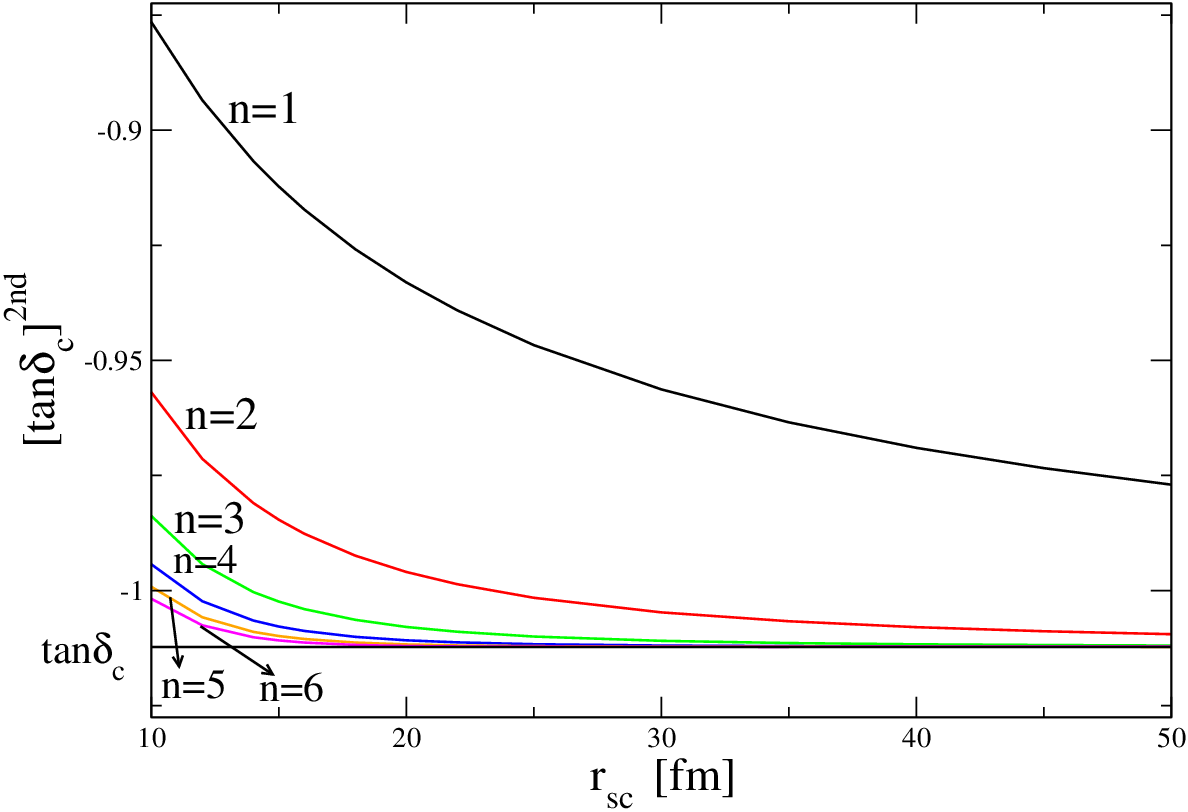
where the unscreened Coulomb potential is included in $H$. This estimate depends on $n$ and $r_{sc}$ as the wave function does. In Fig. 3 the second order estimate $[\tan\delta_{c}]^{2^{nd}}$ is shown as a function of $r_{sc}$ for different values of $n$. The straight line is the exact value of $\tan\delta_{c}$ obtained solving the Schrödinger equation. We can observe that for $n\geq 4$ and $r_{sc}>30$ fm the second order estimate coincides with the exact results. In this example the integral relations derived from the Kohn Variational Principle have been used to extract a phase-shift in the presence of the Coulomb potential using wave functions with free asymptotic conditions.

The integral relations derived from the KVP are general and their validity is not limited to two-body systems. The two-body system is the simplest system in which different applications can be studied and compared to the exact solution of the Schrödinger equation and, therefore, a detailed analysis of the variational character of the relations can be performed. In this section the study of the integral relations is extended to describe a $2+1$ collision in the three-body system, below the breakup threshold into three particles. The description of the breakup channel remains outside the scope of the present work. In the following we will consider the two examples already discussed in the previous section: the computation of phase-shifts using bound state like wave functions and the calculation of phase-shifts in presence of the Coulomb potential using wave functions having free asymptotic conditions. To this end we will use the $s$-wave MT I-III nucleon-nucleon interaction [24], active in the singlet and triplet spin states, respectively:

	$\displaystyle V_{MT\;I}(r)=$	$\displaystyle\frac{1438.72}{r}{\rm e}^{-3.11r}-\frac{513.968}{r}{\rm e}^{-1.55r}$		(34)
	$\displaystyle V_{MT\;III}(r)=$	$\displaystyle\frac{1438.72}{r}{\rm e}^{-3.11r}-\frac{626.885}{r}{\rm e}^{-1.55r}$

with distances in fm and energies in MeV. This interaction has been used many times in the literature to study the three-nucleon system at low energies. It is considered a semi-realistic interaction since it describes reasonably well the deuteron binding energy and the singlet and triplet $n-p$ scattering lengths. Its predictions for these quantities are $E_{d}=-2.23069$ MeV, ${}^{1}a_{n-d}=-23.582$ fm, and ${}^{3}a_{n-d}=5.5132$ fm. To be noticed that this potential has a strong repulsion at short distances.

To compute bound and scattering wave functions we make use of the pair hyperspherical harmonic (PHH) method which has proven to be extremely accurate [18, 25]. In the following a brief illustration of the method is given. For bound states, the three-nucleon wave function is decomposed in three Faddeev-like amplitudes

$$\Psi=\psi({\bm{X}}_{i},{\bm{Y}}_{i})+\psi({\bm{X}}_{j},{\bm{Y}}_{j})+\psi({\bm{X}}_{k},{\bm{Y}}_{k})\;\;,$$

(35)

where we have introduced the Jacobi coordinates: ${\bm{X}}_{i}=({\bm{r}}_{j}-{\bm{r}}_{k})/\sqrt{2}$ and ${\bm{Y}}_{i}=({\bm{r}}_{j}+{\bm{r}}_{k}-2{\bm{r}}_{i})/\sqrt{6}$ (the generic vector ${\bm{r}}_{k}$ indicates the position of nucleon $k$). Each amplitude having quantum numbers $J,J_{z},T,T_{z}$ is expanded in angular-spin-isospin channels (called $\alpha$-channels) as

	$\displaystyle\psi({\bm{X}}_{i},{\bm{Y}}_{i})=$	$\displaystyle\sum_{\alpha}\Phi_{\alpha}(X_{i},Y_{i}){\cal Y}_{\alpha}(jk,i)$		(36)
	$\displaystyle{\cal Y}_{\alpha}(jk,i)=$	$\displaystyle\{[Y_{l_{\alpha}}({\hat{X}}_{i})\otimes Y_{L_{\alpha}}({\hat{Y}}_{i})]_{\Lambda_{\alpha}}[s^{jk}_{\alpha}\otimes\textstyle{\frac{1}{2}}]_{S_{\alpha}}\}_{JJ_{z}}[t^{jk}_{\alpha}\otimes\textstyle{\frac{1}{2}}]_{TT_{z}}$

and the radial amplitudes are expanded in terms of the PHH basis

$$\Phi_{\alpha}(X_{i},Y_{i})=\rho^{l_{\alpha}+L_{\alpha}}f_{\alpha}(\sqrt{2}X_{i})\sum_{K}u_{K}^{\alpha}(\rho)\;^{(2)}P_{K}^{l_{\alpha},L_{\alpha}}(\phi_{i})$$

(37)

where we have introduced the hyperspherical variables, the hyperradius $\rho$ and the hyperangle $\phi_{i}$, defined by the relations $X_{i}=\rho\cos\phi_{i},Y_{i}=\rho\sin\phi_{i}$, and ${}^{(2)}P_{n}^{l_{\alpha},L_{\alpha}}(\phi_{i})$ is a hyperspherical polynomial. The summation is given in terms of the grand angular quantum number $K=2n+l_{\alpha}+L_{\alpha}$. The correlation functions $f_{\alpha}(r)$ are introduced to accelerate the rate of convergence of the expansion. They take into account those configurations in which two nucleons are close to each other. A very convenient choice is to derive the correlation functions from a Schrödinger like equation governed by the two-body potential corresponding to the specific $\alpha$-channel [25].

In the following we consider a three-nucleon system in either the $J=1/2^{+}$ or $J=3/2^{+}$ states with total isospin $T=1/2$. The central character of the MT I-III interaction decouples those channels with different values of $\Lambda_{\alpha}$. Moreover, as the interaction acts only in the $s$-wave, we have $l_{\alpha}=0$. This condition limits the number of channels of the ($\Lambda_{\alpha}=0$) $J=1/2^{+}$ state to two channels, corresponding to $s^{jk}_{\alpha}=0,1$, and to one channel, corresponding to $s^{jk}_{\alpha}=1$, in the case of the ($\Lambda_{\alpha}=0$) $J=3/2^{+}$ state. Finally, following Ref. [26], the hyperradial functions are expanded in terms of Laguerre polynomials

$$u^{\alpha}_{K}(\rho)=\sum_{m=0}^{M-1}A^{\alpha}_{K,m}{\cal L}^{(5)}_{m}(z)\exp{(-z/2)}$$

(38)

with $z=\beta\rho$, and $\beta$ a non linear parameter. We can define a complete antisymmetric three-nucleon state $|\alpha,K,m>$, in terms of which the wave function $\Psi_{n}$ for the $n$-th state results to be

$$\Psi_{n}=\sum_{\alpha,K,m}A^{\alpha,n}_{K,m}|\alpha,K,m>\;\;.$$

(39)

The linear coefficients in the expansion are determined by solving the generalized eigenvalue problem

$$\sum_{\alpha^{\prime},K^{\prime},m^{\prime}}A^{\alpha^{\prime},n}_{K^{\prime},m^{\prime}}<\alpha,K,m|H-E_{n}|\alpha^{\prime},K^{\prime},m^{\prime}>=0\;\;.$$

(40)

The extension of the PHH method to describe scattering states below the deuteron breakup, using the KVP, is straightforward [18, 26]. As for bound states, we limit the discussion to the ($\Lambda_{\alpha}=0$) $J=1/2^{+},3/2^{+}$ states with total isospin $T=1/2$. The $N-d$ scattering wave $\Psi_{k}$ function at the center of mass energy $E=E_{d}+(4/3)(\hbar^{2}/m)k^{2}$, is written as

	$\displaystyle\Psi_{k}=$	$\displaystyle\sum_{\alpha,K,m}A^{\alpha,k}_{K,m}|\alpha,K,m>+|F_{k}>+\tan\delta\;|\tilde{G}_{k}>$		(41)
	$\displaystyle|F_{k}>=$	$\displaystyle\sum_{i}\phi_{d}(X_{i})F_{0}(ky_{i})[s^{jk}\textstyle{\frac{1}{2}}]_{JJ_{z}}[t^{jk}\otimes\textstyle{\frac{1}{2}}]_{TT_{z}}$
	$\displaystyle|\tilde{G}_{k}>=$	$\displaystyle\sum_{i}\phi_{d}(X_{i})f_{reg}(y_{i})G_{0}(ky_{i})[s^{jk}\textstyle{\frac{1}{2}}]_{JJ_{z}}[t^{jk}_{\alpha}\otimes\textstyle{\frac{1}{2}}]_{TT_{z}}\;\;,$

with $\phi_{d}(X_{i})$ the deuteron wave function having spin $s^{jk}=1$ and isospin $t^{jk}=0$. $F_{0},G_{0}$ are proportional to the regular and irregular Bessel functions in the case of $n-d$ scattering or to the regular and irregular Coulomb functions, divided by $ky_{i}$, in the case of $p-d$ scattering. The distance between the nucleon $i$ and the deuteron, formed by nucleons $j,k$, is $y_{i}$ and $f_{reg}(y)=(1-\exp{(-\gamma y)})$ is the chosen regularization factor. In our calculations value of $\gamma=0.25\;$fm^-1 has been found to be appropriate. The coefficients $A^{\alpha,k}_{K,m}$ and the first order estimate of $\tan\delta$ are obtained by solving the following linear system

		$\displaystyle\sum_{\alpha^{\prime},K^{\prime},m^{\prime}}A^{\alpha^{\prime},k}_{K^{\prime},m^{\prime}}<\alpha,K,m|H-E|\alpha^{\prime},K^{\prime},m^{\prime}>+\tan\delta<\alpha,K,m|{\cal G}_{k}>=-<\alpha,K,m|{\cal F}_{k}>$		(42)
		$\displaystyle\sum_{\alpha,K,m}A^{\alpha,k}_{K,m}<\alpha,K,m|{\cal G}_{k}>+\tan\delta<\tilde{G}_{k}|{\cal G}_{k}>=-<\tilde{G}_{k}|{\cal F}_{k}>\;\;,$

where we have defined $|{\cal G}_{k}>=(H-E)|\tilde{G}_{k}>$ and $|{\cal F}_{k}>=(H-E)|F_{k}>$. Following Eq. (21), the second order estimate for $\tan\delta$ is

	$\displaystyle B^{2^{nd}}_{k}$	$\displaystyle=$	$\displaystyle-\frac{m}{\hbar^{2}}<$	$\displaystyle\Psi_{k}|{\cal F}_{k}>$		(43)
	$\displaystyle A_{k}$	$\displaystyle=$	$\displaystyle\frac{m}{\hbar^{2}}<$	$\displaystyle\Psi_{k}|{\cal G}_{k}>$
	$\displaystyle[\tan\delta_{k}]^{2^{nd}}$	$\displaystyle=$		$\displaystyle B^{2^{nd}}_{k}/A_{k}\,\,.$

It should be observed that in the present case, due to the definition of the asymptotic behavior of $\Psi_{k}$, we have $(m/\hbar^{2})<\Psi_{k}|{\cal G}_{k}>=1$.

In Table 2, the ³H and ³He bound states and the doublet and quartet n-d and p-d scattering lengths, corresponding to the MT I-III potential, are given in terms of the number $M$ of Laguerre polynomials used in the expansion of the hyperradial functions. The calculations have been done using $K=16$ which corresponds to 18 (9) hyperradial functions in the case of $J=1/2^{+}$ ($J=3/2^{+}$). With $M=24$, an accuracy better than $1$ keV is obtained for the bound state energies and of the order of $0.001$ fm for the scattering lengths. In Figs. 4 and 5 the $J=1/2^{+},3/2^{+}$, $l=0$, phase shifts $\delta$ are given as a function of the energy in the form of the effective range functions for $n-d$ and $p-d$, respectively. Following Ref. [27], for $n-d$ scattering this function is defined as ($E^{0}=E-E_{d}$)

$$K(E^{0})=k\cot\delta$$

(44)

whereas for $p-d$ scattering it is defined as

$$K(E^{0})=C_{0}^{2}(\eta)k\cot\delta+2k\eta h(\eta)\;\;,$$

(45)

where $\eta$ is the Coulomb parameter, $C_{0}^{2}=2\pi\eta/({\rm e}^{2\pi\eta}-1)$ and $h(\eta)=-{\rm ln}(\eta)+{\rm Re}\psi(1+i\eta)$ ($\psi$ is the digamma function). The solid line in the figures represents these two functions obtained solving Eqs.(42,43) for several values of the center of mass energy $E^{0}$ in the interval $[0,|E_{d}|]$. The solid points in the figures are the results obtained from the integral relations using bound state wave functions as explained below.

The capability of the PHH to produce a very accurate description of bound and scattering states can be used to study different applications of the integral relations. The lowest eigenvalue after the diagonalization procedure of Eq. (40) corresponds to the three-nucleon bound state energy of ³H ($T_{z}=-1/2$) or ³He ($T_{z}=1/2$). However more negative eigenvalues could appear. For example, in the case of $K=16$, $M=24$ and $\beta=1$ fm^-1, six negative eigenvalues $E_{n}$ appear satisfying $|E_{n}|<|E_{d}|$. They are given in Table 3 transformed to the positive energies $E_{n}^{0}=E_{n}-E_{d}$. The corresponding eigenvectors $\Psi_{n}$ approximately describe a scattering process at the center of mass energy $E_{n}^{0}$, though asymptotically they go to zero. In the following we use the index $n$ to label these approximate scattering states and reserve the continuous index $k$ to label those scattering states having the correct asymptotic behavior, as given by Eq. (41). We now consider the diagonalization of the Hamiltonian calculated using the PHH basis with the aforementioned values of $K$, $M$, and $\beta$ but for the $J=3/2^{+}$ state. The $J=3/2^{+}$ state does not have any bound state, however six negative eigenvalues appear, all of them satisfying $|E_{n}|<|E_{d}|$. The positive energies $E_{n}^{0}$ are also given in Table 3. As in the previous case, the corresponding eigenvectors approximately describe the $N-d$ scattering states, though asymptotically they go to zero. It should be observed that changing the values of $K$, $M$ and $\beta$, the number of these states and the corresponding energies at which the eigenvalues appear change. They do not present the stability that a true bound state shows. If we call $E_{0}^{D}$ the bound state energy calculated using a basis of dimension $D$, the variational principle establishes that $E_{0}^{D}\geq E_{3B}$, with $E_{3B}$ the energy corresponding to $D\rightarrow\infty$. When the value of $D$ is sufficiently high, a further increase of the dimension of the basis will not give an appreciable improvement in $E_{0}^{D}$, showing a pattern of convergence of the type given in Table 2. On the other hand, the eigenvalues $E_{n}$ are embedded in the continuum spectrum of $H$ which starts at $E_{d}$. Accordingly, increasing $D$ these eigenvalues tend to $E_{d}$ and the number of them also increases. Similarly to what it has been done in the two-body case, we can consider these states to be approximate solutions of $(H-E_{n})\Psi_{n}=0$ in the interaction region and use them as inputs in the integral relation to compute second order estimates of the phase-shifts. Defining $k^{2}_{n}=(4/3)E_{n}^{0}/(\hbar^{2}/m)$, with $\Psi_{n}$ the corresponding eigenvector and $|F_{n}>,|\tilde{G}_{n}>$ the asymptotic functions of Eq. (41) calculated at $k_{n}$, the second order estimate for the phase shift at each energy is obtained as

	$\displaystyle-$	$\displaystyle\frac{2m}{\hbar^{2}}<\Psi_{n}|H-E_{n}|F_{n}>=B_{n}$		(46)
		$\displaystyle\frac{2m}{\hbar^{2}}<\Psi_{n}|H-E_{n}|\tilde{G}_{n}>=A_{n}$
		$\displaystyle[\tan\delta_{n}]^{2^{nd}}=\frac{B_{n}}{A_{n}}.$

The second order estimates of the phase-shifts for the six cases given in Table 3 are shown in Figs. 4 and 5 as solid points in the effective range functions. We can observe an extremely good agreement with the scattering calculations. This method allows for the calculation of phase-shifts using bound state type functions, even in the case of charged particles. These results can be compared to the analysis of Ref. [27], in which $N-d$ phase-shifts were obtained solving the Faddeev equations in configuration space. For the $n-d$ case, the results presented here and those from Ref. [27] are in complete agreement. In the $p-d$ case the results of Ref. [27] were obtained considering the Coulomb potential in $s$-wave, without including the correction obtained using the KVP as was done in Ref. [16]. In fact, that paper reports the doublet and quartet $p-d$ scattering lengths considering the Coulomb potential in $s$-wave (the given values are $0.16$ fm and $13.75$ fm, respectively). After the correction introduced by using the KVP and considering the complete Coulomb potential, the results from Ref. [16] are $0.003$ fm and $13.95$ fm, respectively. They are in close agreement with the results obtained here and given in Table 2. It is worth noting that the use of the integral relations permits a correct computation of the $p-d$ phase-shifts in the energy range $[0,E_{d}]$, after a diagonalization procedure of the Hamiltonian using square integrable basis functions.

In the last example of this Section, we explore the possibility of extracting $p-d$ phase-shifts from a calculation in which the Coulomb potential has been screened at a certain distance, as we have already done for the two body case. In the three nucleon system, we define the screened Coulomb potential as

$$V_{sc}(i,j)=\left[{\rm e}^{-(r_{ij}/r_{sc})^{n}}\right]\frac{e^{2}}{r_{ij}}(t^{i}_{z}+1/2)(t^{j}_{z}+1/2)$$

(47)

with $r_{ij}$ the interparticle distance between nucleons $(i,j)$. Using the PHH method, we solve a $p-d$ scattering problem using the screened potential and, therefore, the asymptotic behavior is of the form of Eq. (41), with $F_{0}$ and $G_{0}$ the regular and irregular Bessel functions. For different values of $n$ and $r_{sc}$ we calculate the scattering wave function $\Psi^{n,r_{sc}}_{k}$ and, using the integral relations, we determine the Coulomb phase shift. Similarly to what we have done in the two-body case, the integral relations are

	$\displaystyle B^{2^{nd}}_{k}$	$\displaystyle=$	$\displaystyle-\frac{m}{\hbar^{2}}<$	$\displaystyle\Psi^{n,r_{sc}}_{k}|H-E|F_{k}>$		(48)
	$\displaystyle A_{k}$	$\displaystyle=$	$\displaystyle\frac{m}{\hbar^{2}}<$	$\displaystyle\Psi^{n,r_{sc}}_{k}|H-E|{\tilde{G}}_{k}>$
	$\displaystyle[\tan\delta_{c,k}]^{2^{nd}}$	$\displaystyle=$		$\displaystyle B^{2^{nd}}_{k}/A_{k}\,\,.$

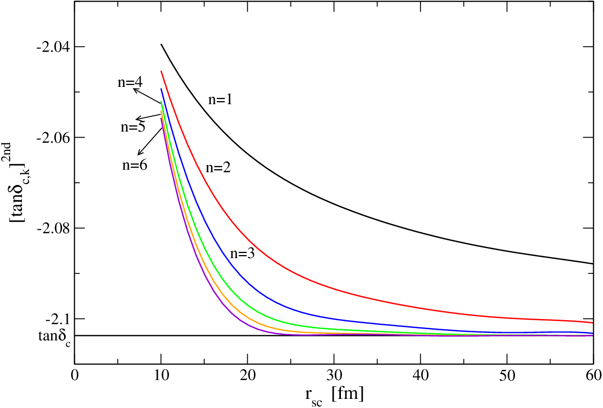
In $H$ the unscreened Coulomb potential is included and the asymptotic functions $F_{k}$ and $\tilde{G}_{k}$ are given in Eq. (41) in terms of the Coulomb functions $F_{0},G_{0}$. The results are shown in Fig. 6 for the case of $J=3/2^{+}$ at $E_{cm}=2$ MeV. The second order estimates [$\tan\delta_{c,k}]^{2^{nd}}$ are given for different values of $n$ as a function of $r_{sc}$. For $n>4$ and $r_{sc}\approx 30$ fm, the results are in complete agreement with the value obtained solving the $p-d$ case without any screening of the Coulomb potential, $\tan\delta_{c}=-2.1037$, which is shown as a straight line in the figure. This method can be compared to the method given in Ref. [20] in which the Coulomb potential was screened using the same screening function as in Eq. (47) and the Coulomb phase shift was recovered after a renormalization procedure. We can conclude that the integral relations used in Eq. (48) produce the same effect as the renormalization procedure.

In order to study applications of the integral relations using the HA method for a three-nucleon system, we give a brief introduction to the method following Refs. [22, 23] (for more details see Ref. [28]). In the HA method the three-body wave function of Eq. (35) is expanded as

$$\Psi=\sum_{\mu=1}^{\infty}w_{\mu}(\rho)\Phi_{\mu}(\rho,\Omega),$$

(49)

where $\Phi_{\mu}(\rho,\Omega)$ is a HA basis element and $[\rho,\Omega]\equiv[\rho,\phi_{i},{\hat{X}}_{i},{\hat{Y}}_{i}]$ is the set of coordinates consisting of the hyperradius and of the five hyperspherical coordinates. The HA basis elements are the eigenfunctions of the hyperangular part of the Hamiltonian at fixed values of $\rho$:

$$\left[\frac{\hbar^{2}}{2m\rho^{2}}G^{2}+V(\rho,\Omega)\right]\Phi_{\mu}(\rho,\Omega)=U_{\mu}(\rho)\Phi_{\mu}(\rho,\Omega)\;\;,$$

(50)

where $G^{2}$ is the grand-angular operator and $V(\rho,\Omega)=\sum_{i}V(X_{i})$ is the potential energy. The eigenvalues, $U_{\mu}(\rho)$, are the adiabatic potentials, that appear in the coupled set of differential equations

	$\displaystyle\left[-\frac{\hbar^{2}}{2m}T_{\rho}+U_{\mu}(\rho)-\frac{\hbar^{2}}{2m}Q_{\mu\mu}(\rho)-E\right]w_{\mu}(\rho)-$
	$\displaystyle\frac{\hbar^{2}}{2m}{\displaystyle\sum_{\mu^{\prime}\neq\mu}^{N_{A}}}\left[Q_{\mu\mu^{\prime}}(\rho)+P_{\mu\mu^{\prime}}(\rho)(\frac{5}{\rho}+2\frac{d}{d\rho})\right]w_{\mu^{\prime}}(\rho)=0$		(51)

with $T_{\rho}=\partial^{2}/\partial\rho^{2}+(5/\rho)\partial/\partial\rho$, $N_{A}$ the number of adiabatic channels included in the calculation, $E$ the three-body energy, and from which the hyperradial functions $w_{\mu}(\rho)$ are obtained. The coupling terms are defined as: $P_{\mu\mu^{\prime}}=<\Phi_{\mu}(\rho,\Omega)|\partial/\partial\rho|\Phi_{\mu^{\prime}}(\rho,\Omega)>$ and $Q_{\mu\mu^{\prime}}=<\Phi_{\mu}(\rho,\Omega)|\partial^{2}/\partial\rho^{2}|\Phi_{\mu^{\prime}}(\rho,\Omega)>$. In Ref. [22] the solution of the system of Eq. (51) has been studied for scattering states below the three-body breakup. In that study it emerged that the use of the integral relations helped to obtain a pattern of convergence for the phase-shift, in terms of the adiabatic channels, similar to the pattern obtained when the HA expansion is used to describe the bound states. It was also shown that the convergence, without the application of the integral relations, is extremely slow. This problem originates in the boundary conditions imposed on the solution of the linear system. As $\rho\rightarrow\infty$ the scattering wave function behaves asymptotically as

$$\Psi_{k}\rightarrow\phi_{d}(r)\left[\frac{\sin{(k_{\rho}\rho)}}{\sqrt{k_{\rho}}\rho}+\tan\delta_{\rho}\frac{\cos{(k_{\rho}\rho)}}{\sqrt{k_{\rho}}\rho}\right]|ST\rangle.$$

(52)

with $|ST>$ the total spin-isospin function and $k^{2}_{\rho}=E^{0}/(\hbar^{2}/2m)=\frac{3}{2}k^{2}$. In fact, when $\rho\rightarrow\infty$, the distance $X_{i}$ is limited by $\phi_{d}$ and $y_{i}=\frac{\sqrt{6}}{2}Y_{i}\rightarrow\frac{\sqrt{6}}{2}\rho$, then the approximate relation $ky_{i}\approx k_{\rho}\rho$ holds. However, the exact equivalence between $ky_{i}$ and $k_{\rho}\rho$ is not matched for any finite value of $\rho$ and, accordingly, the boundary condition of Eq.(52) is equivalent to that of Eq.(41) only at $\rho\approx\infty$ and $N_{A}\rightarrow\infty$. As a consequence $\delta_{\rho}$ converges extremely slowly to $\delta$ by increasing the number of adiabatic states. Therefore, the application of the integral relations in the case of the HA method, as discussed in Ref. [22], removes the limitation given by the slow convergence allowing an accurate description of the scattering states.