The Spatial Clustering of ROSAT All-Sky Survey AGNs
I. The cross-correlation function with SDSS Luminous Red Galaxies
Abstract
We investigate the clustering properties of 1550 broad-line active galactic nuclei (AGNs) at =0.25 detected in the ROSAT All-Sky Survey (RASS) through their measured cross-correlation function with 46000 Luminous Red Galaxies (LRGs) in the Sloan Digital Sky Survey. By measuring the cross-correlation of our AGN sample with a larger tracer set of LRGs, we both minimize shot noise errors due to the relatively small AGN sample size and avoid systematic errors due to the spatially-varying Galactic absorption that would affect direct measurements of the auto-correlation function (ACF) of the AGN sample. The measured ACF correlation length for the total RASS-AGN sample ( erg s-1) is Mpc and the slope . Splitting the sample into low and high samples at erg s-1, we detect an X-ray luminosity-dependence of the clustering amplitude at the 2.5 level. The low sample has Mpc (), which is similar to the correlation length of blue star-forming galaxies at low redshift. The high sample has Mpc (), which is consistent with the clustering of red galaxies. From the observed clustering amplitude, we infer that the typical dark matter halo (DMH) mass harboring RASS-AGNs with broad optical emission lines is log , 11.8, 13.1 for the total, low , and high RASS-AGN samples, respectively.
Subject headings
galaxies: active — large-scale structure of universe — X-rays: galaxiesI. Introduction
Galaxies and active galactic nuclei (AGNs) are not distributed randomly in the universe. The small primordial fluctuations in the matter density field present in the very early universe have progressively grown through gravitational collapse to create the complex network of clusters, groups, filaments, and voids seen in the distribution of structure today. Galaxies and AGNs, as well as groups and clusters of galaxies, are believed to populate the collapsed dark matter halos (DMHs). The clustering of galaxies and AGNs therefore reflects the spatial distribution of dark matter in the universe. This allows clustering measurements to be used to derive cosmological parameters (e.g., peacock_cole_2001; abazajian_zheng_2005). However, these measurements also allow us to study the complex physics which governs the creation and evolution of galaxies and AGNs, as well as the co-evolution of galaxies and AGNs. The co-evolution scenario is motivated by the observed correlation between the mass of the central super-massive black hole (SMBH) and the stellar velocity dispersion in the bulge (gebhardt_bender_2000; ferrarese_merritt_2000), lending strong evidence to an interaction or feedback mechanism between the SMBH and the host galaxy. The specific form of the feedback mechanism, as well as the details of the AGN triggering, accretion, and fueling mechanisms, remains unclear. Different cosmological simulations address possible scenarios for the co-evolution of AGNs and their host galaxies (e.g., kauffmann_haehnelt_2000; dimatteo_springel_2005; cattaneo_dekel_2006). Large volume, high-resolution simulations that include physical prescriptions for galaxy evolution and AGN feedback make predictions for the spatial clustering and large-scale environments of AGNs and galaxies (springel_white_2005; colberg_dimatteo_2008; bonoli_marulli_2009). Observed clustering measurements of AGNs can be used to test these theoretical models, put constraints on the feedback mechanisms, identify the properties of the AGN host galaxies, and understand the accretion processes onto SMBHs and their fueling mechanism.
X-ray surveys allow us to identify AGN activity without contamination from the emission of the host galaxy, i.e., therefore efficiently detecting even low luminosity AGNs. In the current era of deep and wide-area X-ray surveys with extensive spectroscopic follow-up, measurements of the three-dimensional (3D) clustering of AGN in various redshift ranges are emerging (coil_georgakakis_2009; gilli_daddi_2005; yang_mushotzky_2006). However, our knowledge of AGN clustering in the low redshift universe ) is still poor, except for optically selected type II AGNs (wake_miller_2004; li_kauffmann_2006). This is due to the lack of observable comoving volume and the low number density of low- AGNs. Exceptionally large survey areas with good sensitivity are needed to acquire a sufficiently large number of objects for clustering measurements.
To date, the ROSAT All-Sky Survey (RASS; voges_aschenbach_1999) is the most sensitive survey to have mapped the entire sky in X-rays. Surveys with modern higher-sensitivity X-ray observatories such as XMM-Newton and Chandra cover much smaller areas of the sky (area: 0.1-10 deg2). Therefore, the available comoving volume from these deeper data sets is not sufficient to accurately measure AGN clustering at low redshifts ). Serendipitous surveys, such as extended ChAMP (covey_agueros_2008) and 2XMM (watson_schroeder_2009), cover larger areas (33 deg2 and 360 deg2, respectively). However, the large variations in sensitivity between different observations and the non-contiguous sky coverage make serendipitous surveys unsuitable for wide-area clustering measurements.
A few studies have attempted to measure the auto-correlation function (ACF) of RASS-based AGN samples. Two-dimensional (2D) angular correlation functions (akylas_georgantopoulos_2000) do not require redshift measurements for each AGN, but the projection heavily dilutes the clustering signal. Furthermore, the deprojection of the angular clustering to the 3D correlation function is subject to uncertainties in the redshift distribution, which can be substantial. Direct measurements of the 3D RASS-AGN ACF with spectroscopic redshift measurements have been made by [mullis_henry_2004] and [grazian_negrello_2004] with a few hundred AGNs, respectively, providing clustering measurements that have large statistical uncertainties caused by the relatively small sample size.
[anderson_voges_2003, anderson_margon_2007] positionally cross-correlated RASS sources with spectroscopic data available from the Sloan Digital Sky Survey (SDSS). This dramatically increased the number of RASS-AGNs with spectroscopic redshift measurements, which we use here to provide significant improvements in the measurement of AGN clustering at low redshift. Furthermore, the availability of spectroscopic redshifts for large samples of SDSS galaxies in the same volume allows us to use an alternative approach to infer the clustering of AGN using calculations of the AGN–galaxy cross-correlation function (CCF). This approach uses much larger samples of AGN–galaxy pairs and hence significantly reduces the uncertainties in the spatial correlation function compared with direct measurements of the AGN ACF. Furthermore, the use of a CCF avoids the problem that we have to correct for the complex angular dependences of limiting sensitivity in the X-ray sample.
We therefore have initiated a program to investigate the clustering properties of low redshift () RASS-AGNs through measurements of the CCF of these AGNs with SDSS Luminous Red Galaxies (LRGs). In this study, we chose LRGs as the corresponding galaxy sample because they have a significant overlap in redshift range with our X-ray sample (details are described later).
In this first paper of a series, we explain the data selection, as well as the calculation of the CCF and the inferred RASS-AGN ACF. We also investigate the X-ray luminosity dependence of the clustering properties and biases. In a follow-up paper (T. Miyaji et al., in preparation), we will focus on applying the halo occupation distribution (HOD) model to the calculated CCF between RASS-AGNs and LRGs.
The paper is organized as follows. In Section 2, we describe the construction and properties of the LRG and X-ray AGN samples in details. All essential steps to measure the CCF, compute the ACF via the CCF, and estimate errors are explained in Section 3. The results of the clustering measurements for the different X-ray AGN samples and their luminosity dependence are given in Section 4. We discuss these results in Section 5 in the context of other studies and conclude in Section 6. Throughout the paper, all distances, luminosities, and absolute magnitudes are measured in comoving coordinates and given in units of Mpc, where km s-1, unless otherwise stated. We use a cosmology of and (spergel_verde_2003). We use AB magnitudes throughout the paper. All uncertainties represent a 1 (68.3%) confidence interval unless otherwise stated.
II. Data
II.1. SDSS Luminous Red Galaxy Sample
The optical data analyzed in this study are drawn from the SDSS (york_adelman_2000). We use data both from the main galaxy sample, which has a spectroscopic depth of (strauss_weinberg_2002), and the LRG sample, which has a spectroscopic depth of , significantly fainter than the main galaxy sample. The LRG sample was designed for studies of large-scale structure to higher redshift; it covers a larger volume than the main galaxy sample. Here we use the LRG sample as a large-scale structure tracer set to calculate the CCF with the RASS-AGN, as the LRG sample covers a similar redshift range as the RASS-AGNs.
The target selection and the properties of the LRG sample are described in detail in [eisenstein_annis_2001]. Two different selection criteria (’cut I’ and ’cut II’) were introduced in identifying LRGs as at the typical 4000 Å break in the spectral energy distribution (SED) of an early-type galaxy drops out of the band and falls into the band. [eisenstein_annis_2001] shows that up to a volume-limited sample of LRGs with passively evolving luminosity and rest-frame colors is selected with a very high efficiency (95% for cut I and 90% for cut II). [eisenstein_annis_2001] advised that the LRG selection algorithm should not used for objects .
II.1.1 Extraction of the SDSS Luminous Red Galaxy Sample
The LRG sample was obtained using the web-based SDSS Catalog Archive Server Jobs System11 1 http://casjobs.sdss.org/CasJobs/. The appropriate objects are selected through the prime target flag ’galaxy_red’ (eisenstein_annis_2001). In SDSS DR2, the model magnitude code was changed (abazajian_adelman-mccarthy_2004) to improve the star–galaxy separation. This also caused a slight change in the LRG sample definition. We make use of the updated LRG sample selection.
We extract 115,577 LRGs in the DR7 data release that have a spectroscopic redshift of , a galaxy spectral-type classification, and a redshift confidence level of . We discovered that 3% of objects flagged ’galaxy_red’ (i.e., both cut selections) in DR7 do not fall within the LRG selection criteria (see eisenstein_annis_2001). This does not happen in earlier data releases prior to DR7.
To calculate the RASS-AGN–LRG CCF, we wish to define an LRG sample that is both volume-limited and contains a high number density of LRGs to maximize the number of possible AGN–LRG pairs. Table 1 of [zehavi_eisenstein_2005] defines three different volume-limited LRG samples, corresponding to different luminosity ranges, that they use to measure the LRG ACF. The first volume-limited LRG sample, with and , contains the highest number density of objects. Here we adopt the same LRG sample definition, as this sample is the best suited to our scientific goals. We select LRGs from DR7 that meet the criteria of this sample, and we refer to the subsequent data here as ’LRG sample’. We further limited our survey area to DR4+ to match the X-ray sample (see Section II.3). The properties of this sample are shown in Table 1.
The selected LRGs span a range in redshift. To construct a volume-limited sample, one must correct their time-evolving SED to account for the evolution of the stellar population and the redshifting. As described in the Appendix of [eisenstein_annis_2001], we use the extinction corrected magnitude to construct the -corrected and passively evolved rest-frame magnitudes (non-star-forming model). [zehavi_eisenstein_2005] passively evolve their to instead of (eisenstein_annis_2001; we refer to this magnitude by using the notation ). The stellar population synthesis (SPS) code described in [conroy_gunn_2008] is used to derive the purely passive evolution correction. LRGs are brighter at compared to . This value is similar to the one used in [zehavi_eisenstein_2005] who state that the evolution is about 1 mag per unit redshift.
We extensively tested that our LRG sample meet the LRG selection criteria of both [eisenstein_annis_2001] and [zehavi_eisenstein_2005]. We only consider objects that are located in areas of the sky that have a spectroscopic completeness fraction in DR7 of . The vast majority of the objects in our sample (99.9%) belong to the LRG ’cut I’ criteria.
II.1.2 Accounting for the SDSS Fiber Collision
[blanton_lin_2003] describe the algorithm used for positioning tiles in the plane of the sky and assigning spectroscopic fibers for observing objects in the SDSS. The resulting spectroscopic sample of SDSS is spatially biased in that fibers on the same tile cannot be placed closer than 55 arcsec. Spectroscopic redshifts are available for galaxy pairs closer than 55 arcsec only if the field is observed at least twice. As discussed in [zehavi_blanton_2002, zehavi_eisenstein_2005], not taking into account the effects of these fiber collisions would systematically underestimate measured correlation functions, even on large scales. [blanton_schlegel_2005] provide publicly available collision-corrected SDSS catalogs suitable for robust large-scale structure studies. They assign a redshift to a galaxy which has no spectroscopic redshift by giving it the redshift of that galaxy in a galaxy group that is positionally the closest and has a spectroscopic redshift. However, these catalogs are generated only for the main galaxy sample, not the LRG sample.
To correct our LRG sample for fiber collisions, we therefore use the following approach. We select from the SDSS catalog Archive Server all LRG objects that passed the pure photometric-based cut I and cut II selection criteria, with no spectroscopic restrictions applied. Photometrically selected LRGs that get a redshift assigned are only those which have a spectroscopic LRG within a separation of . This corresponds to 2% (1004 objects) of the total LRG sample. Our redshift assignment is a two stage process. First, if the photometrically selected LRG is included in the primary spectroscopic LRG sample but its redshift was initially rejected due to a low confidence level of , the spectroscopic redshift is now accepted independent of its confidence level to correct for fiber collisions. This specific procedure assigns a redshift only to nine objects.
As a next step, we make use of the substantially improved DR7 photometric redshift code (abazajian_adelman-mccarthy_2008) compared to earlier SDSS data releases. If the difference between the spectroscopic redshift () of an LRG and the photometric redshift () of a neighboring (within a 55 arcsecond radius) LRG is
| (1) |
then the photometric LRG is assigned the same redshift as the spectroscopic LRG. Otherwise the photometric redshift is taken to be the correct redshift for the photometric LRG. More than half of all photometric LRG redshifts are assigned the spectroscopic redshift of a neighboring LRG, while the remaining objects are assigned their photometric redshift.
The above procedure for redshift assignment is used because simply adopting the photometric redshift for all objects that do not have a measured spectroscopic redshift would smear out the clustering signal in redshift space and therefore dilute the amplitude of the correlation function. [blanton_lin_2003] verified that for areas of the sky with overlapping spectroscopic tiles, 60% of the galaxies that had a neighboring galaxy within 55 arcsec were within 10 Mpc of the neighbor galaxy. [zehavi_eisenstein_2005] demonstrated that LRGs are highly clustered, so using this procedure for LRGs will result in a higher success rate. The average photometric redshift error () is 2%, and within our sample less than 1% (437 objects) of the LRGs are assigned a photometric redshift.
II.2. The X-ray Sample
The RASS (voges_aschenbach_1999) is currently the most sensitive all-sky survey in the X-ray regime, with a typical flux limit of (0.1-2.4 keV). The area of the sky covered is 99.7%, all of which has at least 50 s of exposure with ROSAT Position Sensitive Proportional Counters (PSPC).
Based on the SDSS data release 5 (DR5), [anderson_margon_2007] classify 6224 AGNs with broad permitted emission lines in excess of 1000 km s-1 FWHM and 515 narrow permitted emission line AGNs matching RASS sources within 1 arcmin (note that 86% of all matches fall within 30). Consequently, broad-line AGNs account for 92% of all RASS/SDSS classifications. In this study, we use the broad emission line RASS-AGNs only. The RASS sources are taken from both the RASS Bright source catalog (voges_aschenbach_1999) and the RASS Faint source catalog (voges_aschenbach_2000) and have a maximum likelihood ML .22 2 [anderson_voges_2003, anderson_margon_2007] say that sources with ML have been included. However, investigating the sample shows that ML has been used. The data cover an area of 5740 deg2. The derived luminosities in [anderson_margon_2007] are based on a flat CDM cosmology with (, , )=(0.3, 0.7, 70 km s-1 Mpc-1).

The RASS/SDSS target selection consists of two selection algorithm: the main SDSS algorithm for galaxies and AGNs () and the specific assignment of SDSS fibers for RASS identifications (). [anderson_voges_2003] explain in detail their selection of optical counterpart candidates.
To understand possible bias effects, which may influence our CCF measurements, we summarize the selection method briefly. The algorithm considers those SDSS optical objects within 1 arcmin of the X-ray source position. Optically detected objects qualify for SDSS spectroscopy if their , , or magnitude is . Since not every optically detected object that fulfills the criteria can be observed spectroscopically, different priority levels are introduced in target selection. The highest priority is given to objects with a triple positional coincidence of RASS X-ray source, SDSS optical object, and FIRST (becker_white_1995) radio source. The next priority level consists of SDSS objects in the RASS error circles with unusual optical colors indicating AGNs (e.g., UV-excess with ). The third priority includes less likely, but plausible, counterparts such as bright stars and galaxies. The last group consists of any object in the magnitude limit that falls within the RASS error circle. One RASS/SDSS spectroscopic fiber is assigned to the object with the highest priority level and a spatial offset less than 27.5 arcsec from the X-ray source. If multiple objects populate the same priority level, one is chosen at random for SDSS spectroscopy.
Before consideration is given to potential RASS targets, an SDSS fiber is first assigned to objects that belong to the main SDSS sample, which includes both galaxies and optically identified AGNs. About 80% of all RASS/SDSS identifications are independently targeted for spectroscopy by the SDSS main target selection algorithm. However, objects in the main sample can be observed at the cost of excluding high-priority RASS targets. In these cases, the RASS/SDSS identification is missing. For these reasons, the RASS/SDSS AGN sample is only reasonably complete (%) for AGNs with .
Objects identified by RASS/SDSS priority levels and not because of their belonging to the main SDSS sample tend to be optically fainter, on average, than the main AGN sample. In the versus color–color space, objects from both selection algorithms lie in the same region. Studying their redshift distributions shows that objects identified by the RASS/SDSS priority levels are, on average, at higher redshifts than the identifications relying on the main SDSS sample. This also explains their lower observed count rates X-ray fluxes. The X-ray hardness ratios of both populations are very similar. Being fainter in X-rays and in the optical wavelengths leads to the same X-ray to optical flux ratio for the RASS/SDSS priority levels AGNs and the main SDSS sample AGNs. Therefore, except that RASS/SDSS priority levels AGNs are found on average at higher redshifts, no intrinsic differences between the RASS/SDSS AGNs from both selection methods are detected.
To create a well-defined X-ray AGN sample to use for clustering measurements, we focus solely on broad emission line AGNs. ROSAT’s sensitivity to the soft energy band that is limited to 2.4 keV selects against X-ray absorbed AGNs (type II), which are usually optically classified as narrow lines objects. Therefore, the sample of broad emission line RASS-AGN is much more complete than the narrow emission line RASS-AGN sample. Furthermore, the X-ray/optical counterpart identification is more reliable for the broad emission line AGNs than for the narrow emission line AGNs, which have much higher surface density (see anderson_voges_2003, anderson_margon_2007 for details).
In addition to studying the clustering of the RASS-AGN sample, here we also test for possible differences in the clustering of low versus high X-ray luminosity RASS-AGN (Figure 1). The commonly used X-ray dividing line between Seyfert AGNs and high luminous QSOs is erg s-1 in the 0.5-10 keV band (intrinsic luminosity; mainieri_bergeron_2002). Although this dividing line is somewhat arbitrary, it is widely employed in literature, and we use it here. [anderson_margon_2007] provide a table which list the galactic absorption-corrected 0.1-2.4 keV luminosities assuming a photon index of . With this index, the AGN/QSO dividing line corresponds to a 0.1-2.4 keV luminosity of log (Figure 1). This index agrees well with that found by [piconcelli_jimenez_2005] in the XMM-Newton spectra of PG quasars in the 0.5-2 keV band, where . In the same paper, it is shown that at higher energies (2-12 keV) the mean photon index for PG quasars gets harder and is . Here we use to be consistent with [anderson_margon_2007].
The properties of our total RASS-AGN sample, low RASS-AGN sample, and the high RASS-AGN sample are shown in Table 1. In order to measure the CCF of the RASS X-ray AGNs with LRGs, the X-ray samples must cover the same area of sky and redshift range as the LRG sample used here. In all samples, no X-ray detected AGN is also classified as an LRG. However, we cannot exclude the possibility that RASS-AGNs are hosted by LRGs and outshine their host galaxies. In contrast to the high RASS-AGN sample, the total RASS-AGN sample and the low RASS-AGN sample are not volume-limited. We calculate the comoving number density in Table 1 of these two samples in the following way. For a specific R.A. and decl. (contained in the DR4+ geometry), we determine the galactic absorption value and the RASS exposure time. The RASS faint source catalog contains sources with at least six source counts. The latter leads to a limiting observable count rate for a given R.A. and decl. Using Xspec, we can compute the Galactic absorption-corrected flux limit versus survey area for the RASS-AGN based on count rates, values, and . We then compute the comoving volume () available to each object () for being included in the sample following [avni_bahcall_1980], using the Galactic absorption-corrected object fluxes from [anderson_margon_2007]. From this we calculate the comoving number density as , where sums over each object.

| Sample | Range | |||||
|---|---|---|---|---|---|---|
| Name | -range | (mag) | Number | ( Mpc-3) | (mag) | |
| LRG sample | 45899 | 0.28 | -21.71 | |||
| -range | Range (erg s-1) | Number | ( Mpc-3) | (erg s-1) | ||
| Total RASS-AGN sample | – | 1552 | 0.25 | |||
| Low RASS-AGN sample | 990 | 0.24 | ||||
| High RASS-AGN sample | 562 | 0.28 |
II.3. Defining a Common Survey Geometry of the RASS-AGN and LRG Samples
The RASS/SDSS [anderson_margon_2007] sample is based on the SDSS DR5, while the LRG sample is drawn from SDSS DR7. We make use of DR7 for the LRG sample as it contains the latest available and furthest advanced version of the SDSS products. Numerous correction have been applied in comparison to earlier data releases (see abazajian_adelman-mccarthy_2008; e.g., updated photo-, repeated observations for few regions with poor seeing in previous data releases, filling holes in DR6 region, correction of instability in the spectroscopic flat-fields). We then limit our LRG sample to the region covered by the [anderson_margon_2007] AGN sample for the CCF calculation.
The SDSS survey geometry and completeness are expressed in terms of spherical polygons (hamilton_tegmark_2004). Publicly available geometry and completeness files are not available for DR5, which would have the largest common survey area between the LRG and the RASS-AGN samples. Therefore, we use the latest version available prior to DR5: the DR4+ geometry file,33 3 http://sdss.physics.nyu.edu/lss/dr4plus, which is a subset (park_choi_2007) of the SDSS DR5 (adelman-mccarthy_agueeros_2007) and covers 5540 deg2 (DR5: 5740 deg2).
The final, fiber collision-corrected LRG sample used here is based on DR7 but reconfigured to include only the DR4+ survey area that has DR7 completeness ratios of . The corresponding area of this sample is 5468 deg2. This reconfiguration of the total [anderson_margon_2007] sample from DR5 to DR4+ eliminates 287 broad emission line objects, leaving 5937 AGNs. Applying the redshift range selection of the LRG sample results in the number of objects given in Table 1 for each AGN sample. Figure 2 shows the sky coverage of our final RASS-AGN sample and the LRG sample reconfigured to a common DR4+ geometry which is used for the calculation of the CCF.
III. Measuring the Cross-correlation Function
A commonly used technique for measuring the spatial clustering of a class of objects is the two-point correlation function (peebles_1980), which measures the excess probability above a Poisson distribution of finding an object in a volume element at a distance from another randomly chosen object:
| (2) |
where is the mean number density of objects. The ACF measures the excess probability of finding two objects from the same sample in a given volume element, while the CCF measures the excess probability finding an object from one sample at a distance from another object drawn from a different sample. The two-point correlation function, , is equal to 0 for randomly distributed objects, and if objects are more strongly clustered than a randomly distributed sample.
In practice, the correlation function is obtained by counting pairs of objects with a given separation and comparing to the number of pairs in a random sample for the same separation. Different correlation estimators are described in the literature. [davis_peebles_1983] give a simple estimator with the form
| (3) |
where is the sum of the data–data pairs at the separation and is the number data–random pairs; both pair counts have been normalized. [landy_szalay_1993] suggest a more advanced estimator:
| (4) |
where is the normalized number of random–random pairs; this estimator yields errors similar to what is expected for Poisson errors only.
Because we measure line-of-sight distances from redshifts, the measurement of is subject to the redshift-space distortions due to peculiar velocities. To separate the effects of redshift distortions, the spatial correlation function is measured as a function of two components of the separation vector between two objects, i.e., one perpendicular to () and the other along () the line of sight. Therefore, is extracted by counting pairs on a 2D grid of separations and . The real-space correlation function can be recovered by integrating along the direction and computing the projected correlation function by [davis_peebles_1983]
| (5) | |||||
which is independent of redshift-space distortions. The variable represents the real-space separation along the line of sight. For a power law correlation function
| (6) |
and are readily extracted from the projected correlation function using the analytical solution
| (7) |
where is the Gamma function.
The aim of this paper is to more accurately measure the clustering properties of low- AGNs than has been measured previously using ACFs (e.g., mullis_henry_2004; grazian_negrello_2004); we accomplish this by measuring the CCF of the AGNs with higher-density LRGs in the same volume. Assuming a linear bias, we follow [coil_georgakakis_2009] and infer the ACF of the AGN sample using
| (8) |
where and are the ACFs of the RASS-AGNs and the LRGs, respectively, and is the CCF of the RASS-AGNs with the LRGs. The LRG ACF is studied extensively in [zehavi_eisenstein_2005], where the estimator in Equation (4) is used; the results are given here in Table 2. The RASS-AGN–LRG CCF is computed here using the estimator given in Equation (3)
| (9) |
We use this estimator as it requires a random catalog for only the LRG sample (), which is homogenous, volume-limited, and has a well-understood selection function. The estimator given in Equation (4) would require a random catalog for the RASS-AGN sample, which would be subject to possible systematic biases due to difficulties in accurately modeling the position-dependent sensitivity limit. Especially, the changing Galactic absorption over the sky causes variations in the flux limit, which would require spectrum-dependent corrections.
III.1. Construction of the Random LRG Sample
The generation of random samples is crucial for a proper measurements of the correlation function. The objective is to construct a sample of randomly distributed sources that have the same observational survey biases as the real sample. Use of the estimator given in Equation (3) requires that the construction of a random sample for only the LRG population is needed.
The LRG sample used here has been corrected for fiber collisions (Section II.1.2); therefore, we do not have to consider this bias in the construction of the random LRG sample. The SDSS survey geometry and completeness ratio for a given field are given by the SDSS geometry files. For a set of random R.A. and decl. values, they allow us to determine if an object is covered by the SDSS DR4+ geometry and the spectroscopic completeness ratio at that location. Only objects covered in DR4+ with a DR7 spectroscopic completeness ratio are accepted for the random sample required here. Additionally, the DR7 spectroscopic completeness is used as the probability that an object is kept for the random sample. If the completeness ratio is 0.9, the object has a 90% chance of being included in the final random LRG sample. This procedure takes into account the fact that survey regions with a high spectroscopic completeness ratio have, on average, a higher object density than less complete areas.
The corresponding redshift for a random object is assigned based on the smoothed redshift distribution of the LRG data sample. The smoothing has been made by applying a least-squares (savitzky_golay_1964) low-pass filter to the observed LRG redshift distribution. We compare the redshift distribution of the LRG data sample, its smoothed profile, and the redshift distribution of the random LRG sample in Figure 3. The shape of the LRG redshift distribution is caused by the superposition of two selection criteria for the LRGs. At low redshifts, most of the LRGs are selected in the SDSS main galaxy sample. This flux-limited selection reaches the maximum at . The ’cut I’ LRG selection provides objects already from the lowest redshifts with a fast increasing number of objects for higher redshifts. This selection reaches its flux limit at . The ’cut II’ selection plays an important role only at . The selection dependence in different redshifts is illustrated in detail in Figure 12–14 of [eisenstein_annis_2001].
The random catalog contains 100 times as many objects as the LRG sample. This value is chosen to have an adequate number of pairs in the sample at the smallest scales measured here.

III.2. Errors and Covariance Matrices
The calculation of realistic error bars on measurements of the correlation function has been a subject of debate since the earliest measurements. Different methods are summarized in [norberg_baugh_2009]. Adjacent bins in are correlated, as are their errors. The construction of a covariance matrix , which reflects the degree to which bin is correlated with bin , is needed to obtain meaningful power law fits to .
We estimate the statistical errors of our correlation measurements using the jackknife method. We divide the survey area into sections, each of which is 55 deg2. We calculate times, where each jackknife sample excludes one section. These jackknife-resampled RASS-AGN ACFs are used to derive the covariance matrix by
| (10) |
where and are from the -th jackknife samples of the RASS-AGN ACF and , are the averages over all of the jackknife samples. The 1 error of each bin is the square root of the diagonal component of this matrix (). To calculate the covariance matrix of the RASS-AGN ACF, which is determined using Equation (8), we compute the RASS-AGN ACF for each of the jackknife samples from the corresponding RASS-AGN–LRG CCF and LRG ACF of each jackknife sample.
III.3. The RASS-AGN Auto-correlation Function
We compute the CCF between RASS-AGNs and LRGs for the total sample, the low sample, and the high sample (see Table 2), as well as the ACF of the LRGs. We measure in a range of 0.3-40 Mpc in 11 bins in a logarithmic scale, while is computed in steps of 5 Mpc in a range of Mpc. The resulting are shown in Figure 4 for Mpc and Mpc. Note the flattened contour at Mpc in the LRG ACF. This is the first direct observation of the coherent infall for LRGs as expected by the Kaiser effect (kaiser_1987).

Although Equation (5) requires an integration over to infinity, in practice an upper bound of integration () is used:
| (11) |
The value of has to be large enough to include most correlated pairs and give a stable solution, but not be so large as to unnecessarily increase the noise in the measurement. To determine the appropriated values for our correlation functions, we determined the correlation length for a set of values by fitting with a fixed over a range of 0.3-40 Mpc.

Figure 5 shows that the LRG ACF saturates at Mpc. The changes in the correlation lengths above this value are well within the uncertainties. Therefore, as in [zehavi_eisenstein_2005], we use an upper bound of the LRG ACF integration of Mpc. Table 2 shows the values of and for a power law fit in a range of 0.3-40 Mpc (as used in zehavi_eisenstein_2005). Both results well agree within their uncertainties.
| Sample | ( Mpc) | |
|---|---|---|
| Our LRG sample | 9.68 | 1.96 |
| Zehavi subsample1 | 9.800.20 | 1.940.02 |
| Total RASS-AGN sample | 6.93 | 1.86 |
| Low RASS-AGN sample | 6.12 | 1.94 |
| High RASS-AGN sample | 7.74 | 1.92 |
Note. — Values of and are obtained from a power law fit to over the range =0.3-40 Mpc for all samples using the full error covariance matrix. For the LRG ACFs, [zehavi_eisenstein_2005] and we used a Mpc, while for all CCFs Mpc was applied.
The CCFs between the different RASS-AGN samples and the LRGs saturate at Mpc (Figure 5). At higher values of , the signal-to-noise ratio degrades and no significant change in occurs. Therefore, we use Mpc as an upper bound of integration for all AGN–LRG CCFs. The difference in the measured LRG ACF using Mpc and Mpc is only 3%. We expect that the growth of the CCF between Mpc and Mpc is about the same order. Since this is much smaller than the errors in the CCF, a use of Mpc for the CCF is reasonable. The correlation length of the CCFs of the different RASS-AGN samples and the LRGs is given in Table 2.
As the area covered by SDSS DR4+ is not contiguous (see Figure 2), we computed the CCF for different subsamples of the SDSS DR4+, to check that there were no biases introduced by using non-contiguous regions of the sky. Excluding survey areas with R.A. and R.A. , the isolated area around R.A. and decl. , the somewhat patchy areas at 190 R.A. and 0 decl. , and combinations thereof, results in measurements of the CCFs that all agree well within their uncertainties. Changing the step size of from 5 to 2.5 Mpc alters by a negligible amount.

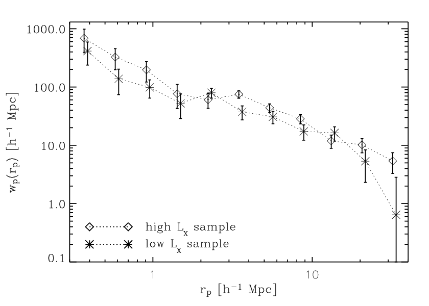
Instead of using the derived values of from the power law fits of the LRG ACF and AGN–LRG CCFs to compute the RASS-AGN ACF, we use Equation (8) and use the full functions. Figure 6 shows for the RASS-AGN ACF, the LRG ACF, and the RASS-AGN–LRG CCF. Figure 7 shows the CCFs for the low and high RASS-AGN samples.
We fit power laws to the ACFs of the different RASS-AGN samples. The fit uses the covariance matrix and minimizes the correlated values according to
| (12) |
We only fit the data in a range 0.3-15 Mpc, as the clustering signal above 15 Mpc is not well-constrained for the low RASS-AGN sample. The upper end of has also been chosen because we will later convert the fit results into which involves only the pairs within 16 Mpc. Contour plots of the resulting values of and are shown in Figure 8 for the different RASS-AGN samples. The derived best-fit values, as well as the best-fit values with a fixed power law slope of , are given in Table III.3. Based on the error on for a fixed , we estimate the clustering signal to be detected at a 11, 5, and 8 level for the total, the low , and the high RASS-AGN sample, respectively. The difference in the clustering signal between the low , and the high RASS-AGN sample is detected at the 2.5 level.

| Sample | log | |||||
|---|---|---|---|---|---|---|
| Name | ( Mpc) | ( Mpc) | () | ( ) | ||
| Total RASS-AGN sample | 4.28 | 1.67 | 4.32 | 0.77 | 1.11 | |
| Low RASS-AGN sample | 3.32 | 1.73 | 3.26 | 0.62 | 0.88 | 11.83 |
| High RASS-AGN sample | 5.44 | 1.86 | 5.52 | 0.98 | 1.44 |