Logarithmic behavior of degradation dynamics in metal–oxide semiconductor devices

The understanding of the physics of semiconductor devices [1] has never been so important, since silicon-based integrated circuits are facing increasing reliability and scaling issues. Quantum Computing [16], DNA Computing [15], and many other alternatives are arising as possible substitutes to the technology of the silicon-based computation, but these seem to be very distant from the reality of our day-by-day.

Hence, the understanding of the reliability effects in semiconductors is of paramount importance for the Microelectronics Industry, that is more and more dependent of new results from an interdisciplinary Physics and their ramifications.

Complementary metal-oxide semiconductors (or simply CMOS devices) have an important role in the development of the information and electronic industry. A scheme of this device can be represented basically by figure 2. As can be observed, it is composed by a thin metal plate, followed by an insulating layer (e.g., SiO₂), and finally a semiconductor layer (Silicon-Si). The working of device supposes two voltages:

1. 1.

   The gate-source voltage ($V_{GS}$), which controls the Fermi-level of charge carriers in the semiconductor, i.e., the electrons are attracted with larger or smaller intensity to the interface between the oxide and semiconductor according to the magnitude of $V_{GS}$;

2. 2.

   The drain source voltage ($V_{DS}$), responsible to move the electrons to compose the current (drain current). The uniformity of this current can be affected by charge traps found close to the semiconductor-insulator interface. In this context the rules of capture and emission of charge carriers by traps in semiconductor devices lead to irregular signals (noise) in the current which can be observed in figure 1.

In this figure we observe how the current of device is affected by a single trap. The fluctuations experimentally observed are caused by the effect of the superposition of a number of traps, under different conditions and moreover, we can consider fluctuations from a sample of devices for completely describing this phenomena (see for example [4]).

Such fluctuations are called random telegraph signals [3]. In other contexts, as for example Ni/NiO/Co junctions [10], such fluctuations are even able to govern magnetoresistance and their study also will be very important in the context of nanostructures (see for example [11], [12]).

The capture and emission of charge carriers by the traps is described as a simple Poisson process governed by rates $\tau_{c}$ and $\tau_{e}$, where the capture occurs with probability $p(0\rightarrow 1)dt=\tau_{c}^{-1}dt$ and and emission $p(1\rightarrow 0)dt=\tau_{e}^{-1}dt$

Such rates $\tau_{c}$ and $\tau_{e}\$can be defined as the time average in state 1 and state 0 respectively: $\tau_{c}=\left\langle t\right\rangle_{1}=\int_{0}^{\infty}t\ P_{1}(t)dt$ and $\tau_{e}=\left\langle t\right\rangle_{0}=\int_{0}^{\infty}t\ P_{0}(t)dt$, where $P_{1}(t)$ is the probability of permanency in state 1 and $P_{0}(t)$ the respective amount for state 0. Naturally $P_{1}(t)=1/\tau_{c}\cdot e^{-t/\tau_{c}}$ and $P_{0}(t)=1/\tau_{e}\cdot e^{-t/\tau_{e}}$.

If the number of trapped charge carriers increases over time, a decrease of the current may be observed. This is an aging effect usually called bias temperature instability (n- or p-bti), since it depends on bias (Fermi level) and temperature, as discussed below.

In this context the degradation of a MOS transistor can be measured as the number of occupied traps and the dynamics of this occupation must be better understood. In this paper we aim at a theoretical analysis to describe the density of occupied traps in a semiconductor device and so to understand how a characteristic degradation process occurs in these devices and other similar devices.

So, first of all, we need to calculate the probability of a particular trap with constants $\tau_{c}$ and $\tau_{e}$ starting from state $0$ (empty) and after a elapsed time $t$ it is in this same state, which we denote $p_{00}(t)$. This probability can be calculated observing that ([1], [3]):

where $p(0\rightarrow 1)=dt/\tau_{c}$ and $\ p(1\rightarrow 1)=1-p(1\rightarrow 0)=1-dt/\tau_{e}$ and also $P_{00}(t)=1-P_{01}(t)$. This leads to a simple differencial equation:$\ dP_{01}(t)/dt=\tau_{c}^{-1}-(\tau_{e}^{-1}+\tau_{c}^{-1})P_{01}(t)$. If $P_{00}(0)=1$, its solution is $P_{01}(t)=\tau_{e}(\tau_{e}+\tau_{c})^{-1}\left[1-\exp(-t/\tau_{eq})\right]$, where $1/\tau_{eq}=1/\tau_{e}+1/\tau_{c}$. Similar results can be performed leading to $P_{11}(t)=\dfrac{\tau_{e}}{\tau_{e}+\tau_{c}}\left[\tau_{e}+\tau_{c}\exp(-t/\tau_{eq})\right]$. Unless fluctuations on the current amplitude, whose average $\Delta$ depends on other microscopic factors of the device, this probability corresponds to the autocorrelation of the system $A(t)=\left\langle\sigma(0)\sigma(t)\right\rangle$, where $\sigma(t)$ corresponds to the state of the trap (occupied $\sigma=0$ or empty $\sigma=1)$. In frequency domain this exponential decay of autocorrelation for one trap is described by Lorentzians, since the power spectrum density, i.e., the fourier transform of the autocorrelation is

The known 1/$f$ noise results from a sum of these Lorentzians (a contribution of the many traps in device). For more details about the origin of 1/$f$ noise, see for example [7],[4], [13], [14].

So, coming back to relaxation phenomena, and starting from $n(0)=0$ (all traps empty), we can calculate the average density of occupied traps at time $t$

where $\Pr(k|n(0),t)$ is the probability of just $k$ traps are occupied at time $t$, with $k=0...N_{tr}$. But the traps have different constants $\tau_{e}$ and $\tau_{c}$ and from that, we write

with $C_{k}$ denoting every subset $\{d_{1},d_{2},...,d_{k}\}$ from $\{1,2,...,,n\}$. But $\left\{\tau_{c}^{(d_{i})},\tau_{e}^{(d_{i})}\right\}_{i=1}^{N_{tr}}$ are statistically independent and identically distributed, and we have :

where $\overline{\cdot}=\int\int\cdot\ f(\tau_{c})g(\tau_{e})d\tau_{c}d\tau_{e}$, where $f(\tau_{c})$ and $g(\tau_{e})$ are probability densities of time constant times of capture and emission. Microscopically these quantities can be better understood. Actually, $\tau_{c}$ and $\tau_{e}$ have a thermal and a gate voltage dependence. Some more detailed approaches use quantum two-dimensional calculations of these quantities [9]. Here we use a known simplification proposed by Kirton and Uren [1], where $\tau_{c}$ and $\tau_{e}$ are random variables that follow the form: $\tau_{c}=10^{p}(1+\exp(-q))$ and $\tau_{e}=10^{p}(1+\exp(q))$, where $p\in[p_{\min},p_{\max}]$ and$\ q=(E_{t}-E_{F})/k_{B}T\in[E_{v}-E_{F})/k_{B}T,(E_{c}-E_{F})/k_{B}T]$ are randomly distributed according to respectively a uniform and a u-shape distribution.

There is no much information about these density of states of the traps in literature, but Wong and Cheng [6] show that for 3 different prepared gate oxides it follows a u-shape form.

Naturally, we must observe that $\tau_{eq}=\tau_{c}\tau_{e}/(\tau_{c}+\tau_{e})=10^{p}$ corresponds to an uniform distribution of time constants ($\tau_{eq}$) in a log scale, as expected. Here, $E_{t}$ and $E_{F}$ are respectively the energy of observed trap and Fermi Level of system that is directly proportional to $V_{GS}$ applied in device. For our purpose, it is more interesting to switch our average:

where $\Omega(E_{t})$ is the density of states of the traps in the interface.

Coming back to equation 1, after some straithforward calculations we have

The second integral must be better worked out. Making a suitable change variable $p=-\log_{10}$ $(\frac{u}{t})$, $dp=-\ln^{-1}10\frac{du}{u}$ and we have the temperature dependence separated of time dependence via two integrals:

which can be analyzed numerically. A particular case is when $f(E_{t})$ is uniform, and in this case we have $\int\nolimits_{E_{v}}^{E_{c}}\frac{dE_{t}\ \Omega(E_{t})}{1+e^{-(E_{t}-E_{F})/k_{B}T}}=\frac{k_{B}T}{(E_{c}-E_{v})}\ln\left[\frac{e^{(E_{c}-E_{v})/k_{B}T}+e^{(E_{F}-E_{v})/k_{B}T}}{1+e^{(E_{F}\ -E_{c})/k_{B}T}}\right]$. If $E_{F}$ $=(E_{v}+E_{c})/2$, i.e., it is exactly in the middle of band gap, this integral is numerically equal $1/2$ and there is no temperature dependence, i.e.,

A simple particular case is if we observe the evolution of the occupation probability of a single trap, with time constants $\tau_{c}$ and $\tau_{e}$, is numerically equal to $\lim_{N_{tr}\rightarrow\infty}$ $\overline{\left\langle n(t)\right\rangle_{uniform}}/N_{tr}$ when all traps have the same $\tau_{e}$ and $\tau_{c}$, which is given by:

where $\beta=\tau_{c}/\tau_{e}$ is a important ratio considered in this context. Naturally $\Pr(\sigma_{i}(t)=1)\rightarrow$ $\frac{1}{1+\beta}=\frac{\tau_{e}}{\tau_{e}+\tau_{e}}$ when $t\rightarrow\infty$. This leads to a simple but important conclusion: if $\beta>1$ (time capture is greater than time emission) we have $\Pr(\sigma_{i}=1)<1/2$ and otherwise – i.e., $\beta<1$(time emission greater than time capture), $\Pr(\sigma_{i}=1)>1/2$ when $t\rightarrow\infty$.

But what is the behavior of $\overline{\left\langle n(t)\right\rangle}$ in a realistic case(i.e., when $\tau_{c}$ and $\tau_{e}$ are randomly distributed)? In this case we solve numerically the exponential integral from 2. We adopt usual values found in the literature for this problem ($p_{\min}=0$ and $p_{\max}=7$) what means a frequency ranging from 1 to 10⁷ Hz.

The continuous curve in figure 3 shows the time evolving $\overline{\left\langle n(t)\right\rangle}$ theoretically obtained (i.e. numerical integration of equation 2).

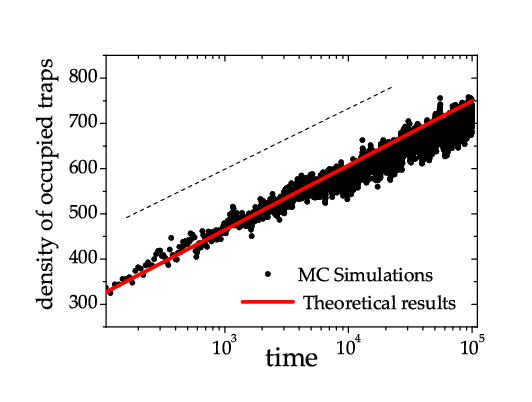
The points corresponds to our MC simulations. For these MC simulations, we start from a given number of empty traps. For each time, each empty trap $i=1,...,N_{tr}$ becomes occupied with probability $p_{i}(0\rightarrow 1)=10^{-p_{i}}(1+e^{-q_{i}})^{-1}$ and similarly an occupied trap becomes empty again with probability $p_{i}(1\rightarrow 0)=10^{-p_{i}}(1+e^{q_{i}})^{-1}$, where $p_{i}$ is uniformly drawn in $[p_{\min},p_{\max}]$, and here the same values ($p_{\min}=0$ and $p_{\max}=7$) were used. Similarly $E_{t}^{(i)}$is uniformly drawn in $[E_{v},E_{c}]$. For real devices $E_{t}$ should change from $\ \char 126\relax\ 0.2\$eV to $\ \char 126\relax\ 1.0$ eV. First of all, $E_{F}$ corresponds to middle of band-gap ($E_{F}\ \char 126\relax\ 0.6\$eV$)$, $k_{B}=8.617385\times 10^{-5}$eV K^-1and $T=300$ K, which leads to $q_{i}\in[-15.473,15.473]$. We can observe a excellent agreement between the MC simulations and our theoretical equations, showing that in semi-log plot in figure 3 the relaxation dynamics follows a logarithm law:

where we find $A=31.80(15)$ and $B=144.20(3)$. The uncertainties were obtained, using error bars obtained from 16 independent runs of the program. We test other temperature values but we did not find difference as expected when $E_{F}$ is in the middle of band gap in this case where a uniform density of states is considered.

Extending our results, we can compute the second moment:

which yields $\overline{\left\langle n(t)^{2}\right\rangle}=N_{tr}\overline{\Pr(k|n(0),t)}+N_{tr}(N_{tr}-1)\overline{\Pr(k|n(0),t)}^{2}\approx\overline{\left\langle n(t)\right\rangle}+\overline{\left\langle n(t)\right\rangle}^{2}$

So we have $\left\langle n(t)^{2}\right\rangle\approx\frac{N_{tr}\ln^{-1}10}{2(p_{\max}-p_{\min})}\int\nolimits_{10^{-p_{\min}}t}^{10^{-p\max}t}du\frac{\left(e^{-u}-1\right)}{u}+\frac{\ln^{-2}10N_{tr}^{2}}{4(p_{\max}-p_{\min})^{2}}\left[\int\nolimits_{10^{-p_{\min}}t}^{10^{-p\max}t}du\frac{\left(e^{-u}-1\right)}{u}\right]^{2}$, which leads to

with $A$ and $B$ exactly as reported before.

Looking at the temperature dependence, we must analyze more realistic densities of states. After a detailed scanning of the plots for the densities of states, for the 3 prepared gate oxides (TCE Oxide, Reoxidized Nitrided-oxide, and Nitrided-oxide) found in the reference [6], a fitting by a eighty-degree polynomial, here described by $\widehat{\Omega}(E_{t})=\sum\nolimits_{k=0}^{8}\beta_{k}E_{t}^{k}$ were performed (see [2] for a more detailed discution of this part). This excelent fit can be seen in figure 4.

Using these u-shaped densities of states or even their polynomial fit, we can calculate the temperature dependence:

with $Z=\sum\nolimits_{k=0}^{8}\beta_{k}(k+1)^{-1}(E_{c}^{k+1}-E_{v}^{k+1})$ where then $\overline{\left\langle n(t)\right\rangle}$ $\sim\ \varphi(T,E_{F})(A+B\log t),$ showing that temperature and Fermi level dependence are independent of time, i.e., the relaxation depends logarithmically on time for each fixed pair ($T,E_{F}$).

Using Simpson numerical integration, we calculate $\varphi(T)$ and now the time evolving of $\overline{\left\langle n(t)\right\rangle}$ is calculated according to equation 2. By motivations from experimental results, initially we study $\overline{\left\langle n(t)\right\rangle}$ for a Fermi level set on $E_{F}=Ec=1$eV using the u-shape obtained from Reoxidized Nitrided-oxide.

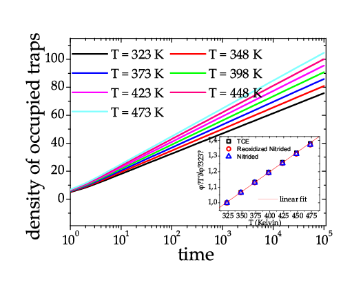
The figure 5 shows $\overline{\left\langle n(t)\right\rangle}$ for different temperatures. The inside plot in this same figure shows the amplification factor of temperature $A(t)=\varphi(T)/\varphi(323)$, since $T_{0}=323$K ($50^{0}$C) is the minimum temperature used in our calculations, for the 3 different oxides extracted from [6]. We show the linear universal behavior, described by relation

It is also interesting to study the dependence on Fermi level. The Fermi level may be varied by changing the gate bias of the device as experimentally explored in [5]. We studied the dependence of $\varphi(T)$ as function of $T$ for different values of $E_{F}$. Our results show that the curves showing the evolution of relaxation as function of time can be collapsed in a single one if multiplied by a suitable constant. This constant is $\varphi(T,E_{F})$ (see figure 6). Hence, our results are in agreement to the experimental findings for the Fermi-level dependence of the relaxation.

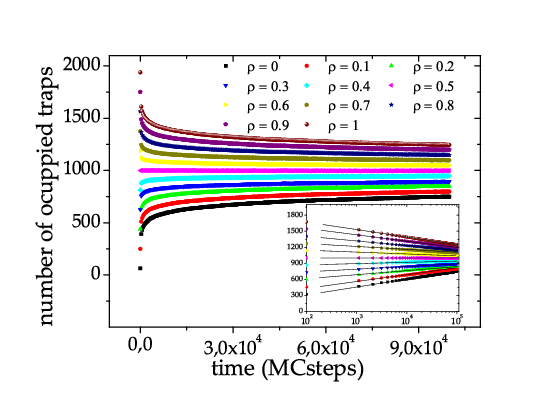
We did also study the dependence on the initial density of occupied traps. In this case, if the density of initially occupied traps is lower than the equilibrium value, in the relaxation process, the number of occupied traps increases logarithmically. On the other hand, if the density of initially occupied traps is higher than the equilibrium value, the density of occupied states decreases logarithmically in the relaxation process. MC simulation did confirm this behavior. MC simulations were performed starting from different initial density of occupied traps $\rho_{0}=0,\ 0.1,\ 0.2,\ 0.3,\ ...,\ 1.0$, where the equilibrium value is $\rho=0.5$. We can observe this behavior in figure 7.

In summary our results corroborate the experimentally observed logarithmic relaxation of the density of the occupied traps via MC simulations and from theoretical analysis in complementary metal-oxide semiconductors governed by Fermi-Dirac-Shockley-Read Statistics [8]. Our results also corroborate the experimentally observed temperature dependence, which shows that the relaxation as a function of time at different temperatures may be collapsed into a single curve using a suitable scaling factor. This behavior is experimentally observed e.g. in [5]. The scaling factor is the function $\varphi(T,E_{F})$ of equation 6.

References

- [1] M.J. Kirton, M.J. Uren, Advances in Physics 38, 4, 367-468 (1989)
- [2] R.da Silva, G.I.Wirth, L.Brusamarello, Journal of Statistical Mechanics: Theory and Experiment, P10015/1-P10015/10 (2008).
- [3] S. Machlup, J. Applied Physics 35, 3, 341-343 (1954)
- [4] R. da Silva, G. I. Wirth, R. Brederlow, Physica A 362, 277-288 (2006)
- [5] T. Grasser, B. Kaczer, IEEE Transactions on Electron Devices, 56(5), 1056-1062 (2009)
- [6] H. Wong, Y. C. Cheng, IEEE Transactions on Electron Devices, 37(7), 1743-1749 (1990)
- [7] B. Kaulakys, T. Meskauskas, Physical Review E, 58(6), 7013-7019 (1998)
- [8] W. Shockley, W. T. Read Jr., Physical Review, 87(5), 835-842 (1952)
- [9] A. Palma, A. Godoy, J. A. Jimenez-Tejada, J. E. Carceller, and J. A. Lopez-Villanueva, Physical Review B, 56(15), 9565-9574 (1997)
- [10] B. Doudin, G. Redmond, S. E. Gilbert, J.-Ph. Ansermet, Phys. Rev. Lett., 79(5), 933–936, (1997)
- [11] W. J. Skocpol, P. M. Mankiewich, R.E. Howard, L. D. Jackel, D. M. Tennant, A. D. Stone, Phys. Rev. Lett., 56(26), 2865–2868 (1986)
- [12] C. Dekker, A. J. Scholten, F. Liefrink, R. Eppenga, H. van Houten, C.T. Foxon, Phys. Rev. Lett., 66(16), 2148-2151 (1991)
- [13] K. S. Ralls, W.J. Skocpol, L. D. Jackel, R. E. Howard, L. A. Fetter, R.W. Epworth, D. M. Tennant, Phys. Rev. Lett., 52(3), 228–231 (1984)
- [14] C. T. Rogers, R. A. Buhrman, Phys. Rev. Lett., 53 (13), 1272–1275 (1984)
- [15] L. M. Adleman, Science 266 (11), 1021–1024 (1994)
- [16] R. Feynman, International Journal of Theoretical Physics 21, 467-488 (1982).