Majorana bound states without vortices in topological superconductors with electrostatic defects
Abstract
Vortices in two-dimensional superconductors with broken time-reversal and spin-rotation symmetry can bind states at zero excitation energy. These socalled Majorana bound states transform a thermal insulator into a thermal metal and may be used to encode topologically protected qubits. We identify an alternative mechanism for the formation of Majorana bound states, akin to the way in which Shockley states are formed on metal surfaces: An electrostatic line defect can have a pair of Majorana bound states at the end points. The Shockley mechanism explains the appearance of a thermal metal in vortex-free lattice models of chiral p-wave superconductors and (unlike the vortex mechanism) is also operative in the topologically trivial phase.
pacs
73.20.At, 73.20.Hb, 74.20.-z, 74.25.fcTwo-dimensional superconductors with spin-polarized-triplet, p-wave pairing symmetry have the unusual property that vortices in the order parameter can bind a nondegenerate state with zero excitation energy [1, 2, 3, 4]. Such a midgap state is called a Majorana bound state, because the corresponding quasiparticle excitation is a Majorana fermion — equal to its own antiparticle. A pair of spatially separated Majorana bound states encodes a qubit, in a way which is protected from any local source of decoherence [5]. Since such a qubit might form the building block of a topological quantum computer [6], there is an intensive search [7, 8, 9, 10, 11, 12] for two-dimensional superconductors with the required combination of broken time-reversal and spin-rotation symmetries (symmetry class D [13]).
The generic Bogoliubov-De Gennes Hamiltonian of a chiral p-wave superconductor is only constrained by particle-hole symmetry, . At low excitation energies (to second order in momentum ) it has the form
| (1) |
for a uniform (vortex-free) pair potential . The electrostatic potential (measured relative to the Fermi energy) opens up a band gap in the excitation spectrum. At the superconductor has a topological phase transition (known as the thermal quantum Hall effect) between two localized phases, one with and one without chiral edge states [14, 15, 16, 17].

Our key observation is that the Hamiltonian (1) on a lattice has Majorana bound states at the two end points of a linear electrostatic defect (consisting of a perturbation of on a string of lattice sites). The mechanism for the production of these bound states goes back to Shockley [18]: The band gap closes and then reopens upon formation of the defect, and as it reopens a pair of states splits off from the band edges to form localized states at the end points of the defect (see Fig. 1). Such Shockley states appear in systems as varied as metals and narrow-band semiconductors [19], carbon nanotubes [20], and photonic crystals [21]. In these systems they are unprotected and can be pushed out of the band gap by local perturbations. In a superconductor, in contrast, particle-hole symmetry requires the spectrum to be symmetric, so an isolated bound state is constrained to lie at and cannot be removed by any local perturbation.
We propose the name Majorana-Shockley (MS) bound state for this special type of topologically protected Shockley states. Similar states have been studied in the context of lattice gauge theory by Creutz and Horváth [22, 23], for an altogether different purpose (as a way to restore chiral symmetry in the Wilson fermion model of QCD [24]).
Consider a square lattice (lattice constant ), at uniform potential . The Hamiltonian (1) on the lattice has dispersion relation
| (2) |
(We have defined the energy scales , .) The spectrum becomes gapless for , , and , signaling a topological phase transition [25]. The number of edge states is zero for and , while it is unity otherwise (with a reversal of the direction of propagation at ). The topologically nontrivial regime is therefore reached for negative but larger than .

We now introduce the electrostatic line defect by changing the potential to on the lattice points at , . In Figs. 1 and 2 we show the closing and reopening of the band gap as the defect is introduced, accompanied by the emergence of a pair of states at zero energy. The eigenstates for which the gap closes and reopens have wave vector parallel to the line defect equal to either or (in the limit when is a good quantum number).
We have calculated that the gap closing at happens at a critical potential given by [26]
| (3) |
The critical potential for closing of the gap at is obtained from Eq. (3) by the replacement of with . The MS states appear for defect potentials in between two subsequent gap closings, as indicated in the inset of Fig. 2.
We conclude that MS states exist for any value of . In contrast, Majorana bound states in vortices exist only in the topologically nontrivial regime [3, 27]. The index theorem [28] for the production of zero-energy modes by the vortex mechanism, which requires the topologically nontrivial phase, is therefore not applicable to the Shockley mechanism.

Our reasoning so far has relied on the assumption of a constant pair potential , unperturbed by the defect. In order to demonstrate the robustness of the Majorana-Shockley mechanism, we have performed numerical calculations that determine the pair potential self-consistently by means of the gap equation [26, 29]. In Fig. 3 we show a comparison of the closing and reopening of the band gap as obtained from calculations with and without self-consistency, in the relevant weak pairing regime (). The self-consistency does not change the qualitative behavior. In particular, the gap only closes at for the parameters chosen (c.f. inset in Fig. 2) and the self-consistent determination of only shifts the critical potential slightly.
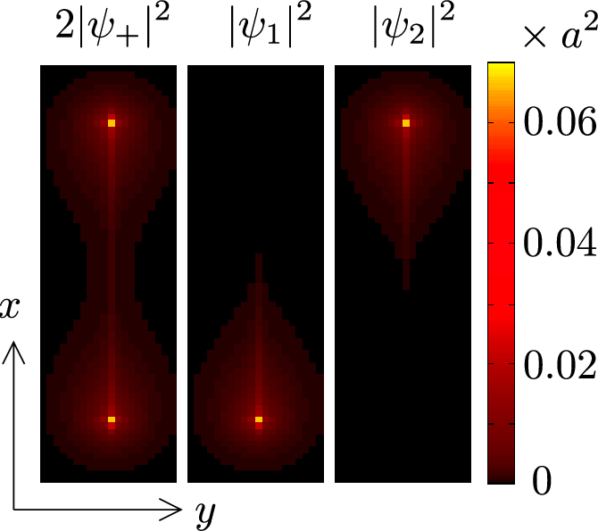
In Fig. 4 we demonstrate that the MS states are localized at the end points of the line defect. The exponentially small, but nonzero overlap of the pair of states displaces their energy from to (with corresponding eigenstates related by particle-hole symmetry). The unpaired Majorana bound states and are given by the linear combinations
| (4a) | ||||
| (4b) | ||||
shown also in Fig. 4. These states are particle-hole symmetric, , so the quasiparticle in such a state is indeed equal to its own antiparticle (hence, it is a Majorana fermion).

If the line defect has a width which extends over several lattice sites, multiple gap closings and reopenings appear at upon increasing the defect potential to more and more negative values at fixed positive background potential . In the continuum limit , the gap closes when [26] , , with the real part of the transverse wave vector and a phase shift that depends weakly on the potential. (Similar oscillatory coupling energies of zero-modes have been found in Refs. [30, 31].) The MS states at the two ends of the line defect alternatingly appear and disappear at each subsequent gap closing.
So far we constructed MS states for a linear electrostatic defect. More generally, we expect a randomly varying electrostatic potential to create a random arrangement of MS states. To test this, we pick at each lattice point uniformly from the interval and calculate the average density of states . The result in Fig. 5 shows the expected peak at . This peak is characteristic of a thermal metal, studied previously in models where the Majorana bound states are due to vortices [32, 33, 34]. The theory of a thermal metal [15] predicts a logarithmic profile, , for the peak in the density of states, which is consistent with our data.
Without Majorana bound states, the chiral p-wave superconductor would be in the thermal insulator phase, with an exponentially small thermal conductivity at any nonzero [3, 32, 35, 36]. Our findings imply that electrostatic disorder can convert the thermal insulator into a thermal metal, thereby destroying the thermal quantum Hall effect. Numerical results for this insulator-metal transition will be reported elsewhere [37].
These results are all for a specific model of a chiral p-wave superconductor. We will now argue that our findings are generic for symmetry class D (along the lines of a similar analysis of solitons in a polymer chain [38]). Let be the momentum along the line defect and a parameter that controls the strength of the defect. Assume that the gap closes at and at . (Because of particle-hole symmetry the gap can only close at or and these two cases are equivalent.) For near and near the Hamiltonian in the basis of left-movers and right-movers has the generic form
| (5) |
with velocities . No other terms to first order in and are allowed by particle-hole symmetry, .
The line defect is initially formed by letting depend on on a scale much larger than the lattice constant. We set one end of the defect at and increase from to . Integration of then gives the wave function of a zero-energy state bound to this end point,
| (6) |
This is one of the two MS states, the second being at the other end of the line defect. We may now relax the assumption of a slowly varying , since a pair of uncoupled zero-energy states cannot disappear without violating particle-hole symmetry.
We conclude with an outlook. We have identified a purely electrostatic mechanism for the creation of Majorana bound states in chiral p-wave superconductors. The zero-energy (mid-gap) states appear in much the same way as Shockley states in non-superconducting materials, but now protected from any local perturbation by particle-hole symmetry. An experimentally relevant consequence of our findings is that the thermal quantum Hall effect is destroyed by electrostatic disorder (in marked contrast to the electrical quantum Hall effect). A recent proposal to realize Wilson fermions in optical lattices [39] also opens the possibility to observe Majorana-Shockley states using cold atoms.
Our analysis is based on a generic model of a two-dimensional class-D superconductor (broken time-reversal and spin-rotation symmetry). An interesting direction for future research is to explore whether Majorana-Shockley bound states exist as well in the other symmetry classes [13]. Since an electrostatic defect preserves time-reversal symmetry, we expect the Majorana-Shockley mechanism to be effective also in class DIII (when only spin-rotation symmetry is broken). That class includes proximity-induced s-wave superconductivity at the surface of a topological insulator [40] and other experimentally relevant topological superconductors [41, 42, 43].
It would also be interesting to investigate the braiding of two electrostatic defect lines, in order to see whether one obtains the same non-Abelian statistics as for the braiding of vortices [4].
We have benefited from discussions with B. Béri, L. Fu, and C.-Y. Hou. This research was supported by the Deutscher Akademischer Austausch Dienst DAAD, by the Dutch Science Foundation NWO/FOM, by an ERC Advanced Investigator Grant, and by the EU network NanoCTM.
References
- [1] N. B. Kopnin and M. M. Salomaa, Phys. Rev. B 44, 9667 (1991).
- [2] G. E. Volovik, JETP Lett. 70, 601 (1999).
- [3] N. Read and D. Green, Phys. Rev. B 61, 10267 (2000).
- [4] D. A. Ivanov, Phys. Rev. Lett. 86, 268 (2001).
- [5] A. Yu. Kitaev, Phys. Usp. 44 (suppl.), 131 (2001).
- [6] C. Nayak, S. Simon, A. Stern, M. Freedman, and S. Das Sarma, Rev. Mod. Phys. 80, 1083 (2008).
- [7] C. Kallin and A. J. Berlinsky, J. Phys. Cond. Matter 21, 164210 (2009).
- [8] S. Tewari, S. Das Sarma, C. Nayak, C. Zhang, and P. Zoller, Phys. Rev. Lett. 98, 010506 (2007).
- [9] M. Sato, Y. Takahashi, and S. Fujimoto, Phys. Rev. Lett. 103, 020401 (2009).
- [10] J. D. Sau, R. M. Lutchyn, S. Tewari, and S. Das Sarma, Phys. Rev. Lett. 104, 040502 (2010).
- [11] P. A. Lee, arXiv:0907.2681.
- [12] J. Alicea, Phys. Rev. B 81, 125318 (2010).
- [13] A. Altland and M. R. Zirnbauer, Phys. Rev. B 55, 1142 (1997).
- [14] G. E. Volovik, JETP Lett. 67, 1804 (1988); JETP Lett. 66, 522 (1997).
- [15] T. Senthil and M. P. A. Fisher, Phys. Rev. B 61, 9690 (2000).
- [16] A. Vishwanath, Phys. Rev. Lett. 87, 217004 (2001).
- [17] G. E. Volovik, The Universe in a Helium Droplet (Clarendon, Oxford, 2003).
- [18] W. Shockley, Phys. Rev. 56, 317 (1939).
- [19] S. G. Davison and M. Stȩślicka, Basic Theory of Surface States (Oxford University, Oxford, 1996).
- [20] A. V. Savin and Y. S. Kivshar, Appl. Phys. Lett. 94, 111903 (2009).
- [21] N. Malkova, I. Hromada, X. S. Wang, G. Bryant, and Z. G. Chen, Opt. Lett. 34, 1633 (2009).
- [22] M. Creutz and I. Horváth, Phys. Rev. D 50, 2297 (1994).
- [23] M. Creutz, Rev. Mod. Phys. 73, 119 (2001).
- [24] K. G. Wilson, Phys. Rev. D 10, 2445 (1974).
- [25] X.-L. Qi, Y.-S. Wu, and S.-C. Zhang, Phys. Rev. B 74, 085308 (2006).
- [26] See EPAPS Document No. XXX for details of the calculation. For more information on EPAPS, see http://www.aip.org/pubservs/epaps.html..
- [27] V. Gurarie and L. Radzihovsky, Phys. Rev. B 75, 212509 (2007).
- [28] R. Roy, arXiv:1001.2571.
- [29] A. Furusaki, M. Matsumoto, and M. Sigrist. Phys. Rev. B 64, 054514 (2001).
- [30] M. Cheng, R. M. Lutchyn, V. Galitski, and S. Das Sarma, Phys. Rev. Lett. 103, 107001 (2009).
- [31] C.-X. Liu, H. Zhang, B. Yan, X.-L. Qi, T. Frauenheim, X. Dai, Z. Fang, and S.-C. Zhang, Phys. Rev. B 81, 041307 (2010).
- [32] M. Bocquet, D. Serban, and M. R. Zirnbauer, Nucl. Phys. B 578, 628 (2000).
- [33] J. T. Chalker, N. Read, V. Kagalovsky, B. Horovitz, Y. Avishai, and A. W. W. Ludwig, Phys. Rev. B 65, 012506 (2001).
- [34] A. Mildenberger, F. Evers, A.D. Mirlin, and J. T. Chalker, Phys. Rev. B 75, 245321 (2007).
- [35] N. Read and A. W. W. Ludwig, Phys. Rev. B 63, 024404 (2000).
- [36] J. H. Bardarson, M. V. Medvedyeva, J. Tworzydło, A. R. Akhmerov, and C. W. J. Beenakker, Phys. Rev. B 81, 121414(R) (2010).
- [37] M. V. Medvedyeva, J. Tworzydło, and C. W. J. Beenakker, arXiv:1004.1111.
- [38] R. Jackiw and G. Semenoff, Phys. Rev. Lett. 50, 439 (1983).
- [39] A. Bermudez, L. Mazza, M. Rizzi, N. Goldman, M. Lewenstein, and M. A. Martin-Delgado, arXiv:1004.5101.
- [40] L. Fu and C. L. Kane, Phys. Rev. Lett. 100, 096407 (2008).
- [41] X.-L. Qi, T. L. Hughes, S. Raghu, and S.-C. Zhang, Phys. Rev. Lett. 102, 187001 (2009).
- [42] S. Ryu, A. P. Schnyder, A. Furusaki, and A. W. W. Ludwig, arXiv:0912.2157.
- [43] L. Fu and E. Berg, arXiv:0912.3294.
Appendix A Line defect in lattice fermion models
We calculate the closing and reopening of the excitation gap upon introduction of a line defect in a lattice fermion model with particle-hole symmetry. First we treat the Wilson fermion model [24] considered in the main text, and introduced in the context of topological insulators in Refs. [1, 2]. Then, in order to demonstrate the generic nature of the results, we consider an alternative lattice model, the staggered fermion (or Kogut-Susskind) model [3, 4, 5], introduced in the context of graphene in Refs. [6, 37].
A.1 Wilson fermions
The Wilson fermion model has Hamiltonian
| (7) |
Each site on a two-dimensional square lattice (lattice constant ) has electron and hole states and . Fermion annihilation operators for these two states are collected in a vector . States on the same site are coupled by the potential matrix and states on adjacent sites by the hopping matrix , defined by [1, 2]
| (8) |
Here is the electrostatic potential on site and is the angle between the vector and the positive -axis (so ). In the continuum limit , the tight-binding Hamiltonian (7) is equivalent to the chiral p-wave Hamiltonian (1), with and .
It is convenient to transform from position to momentum representation. For that purpose we take periodic boundary conditions in the -direction, so that the transverse wavevector (in units of ) has the discrete values , (for an odd number of sites in the -direction). The Fourier transformation from position to momentum representation is carried out by the unitary matrix with elements . We take an infinitely long system in the -direction, so the longitudinal wavevector varies continuously in the interval .
For a uniform potential, for all , the Fourier transformed Hamiltonian has matrix elements
| (9) | ||||
| (10) |
The corresponding dispersion relation is
| (11) |
cf. Eq. (2).
A line defect at row (parallel to the -axis) adds to the perturbation
| (12) |
The determinantal equation for eigenenergy reads
| (13) |
in terms of an matrix with elements . Sylvester’s theorem, , allows us to rewrite the determinant in the form
| (14) |
which reduces to
| (15) |
A zero-mode is a pair of states (one left-mover and one right-mover) at energy . This can only occur at or (because for any eigenenergy at there must also be an eigenenergy at ). From Eqs. (10) and (15) we obtain the condition for such a zero-mode,
| (16) |
where if and if . In the limit we may replace the sum by an integral, , which can be evaluated by contour integration. The resulting critical value of is given in the main text [Eq. (3) and following].
A.2 Staggered fermions
The staggered fermion model is a discretization of the Hamiltonian (1) without the term. It is formulated in Refs. [4, 5, 6] in terms of the transfer matrix , which relates the transverse wave functions at columns and (parallel to the -axis). For a line defect along the -axis, the transfer matrix is -independent, so we can omit the column number .
The transfer matrix (at energy ) has the form
| (17) | ||||
| (18) |
In reference to Eq. (1), the parameter for lattice constant . The matrices and have nonzero elements
| (19) | ||||
| (20) |
while the potential matrix (for a line defect at row ) is given by
| (21) |
In momentum representation, the matrix has elements
| (22) |
where we have defined
| (23) | ||||
| (24) |
The dispersion relation of the staggered fermions is , with
| (25) |
An eigenstate at energy and longitudinal wavevector is an eigenstate of with eigenvalue . The determinantal equation can again be simplified using Sylvester’s theorem. The result, analogous to Eq. (15), is
| (26) |

Because of the pole in the dispersion relation at , the zero-mode now exists only at . The condition for this zero-mode, analogous to Eq. (16), is
| (27) |
For we may again transform the sum into an integral, and thus obtain the critical potential
| (28) |
Upon varying the potential of the line defect, at fixed bulk potential , the closing and reopening of the gap thus happens at (see Fig. 6). The inset shows the region in parameter space where the Majorana-Shockley states exist in the staggered fermion model. This phase diagram is much simpler than the corresponding phase diagram for Wilson fermions (Fig. 2, inset), because of the absence of the extra parameter (which quantifies the strength of the term in the Wilson fermion model).
Appendix B Self-consistent determination of the pair potential
In order to determine the pair potential self-consistently in a spatially non-homogeneous situation, it is necessary to allow for a position-dependent, anisotropic pair potential . The Hamiltonian then reads [29]
| (29) |
where denotes the anticommutator. In the discretization of this Hamiltonian on a square lattice, the spatial dependence of is taken into account in the hopping between neighbors as an average value of on the two lattice points.
When the pair potential is homogeneous, the lattice Hamiltonian has the spectrum
| (30) |
with , and .
The Hamiltonian must be solved self-consistently together with the equation for the pair potential. These read [29] (with derivatives discretized on the lattice)
| (31) |
Here and are the electron and hole component of the wave function, respectively, and assumed to be from the tight-binding model, i.e. they are dimensionless and represent the probability amplitude per lattice point .
The coupling constant must be chosen such that it gives the correct pair potential in the bulk. It can be calculated as
| (32) |
where and are the electron and hole coefficients of the plane wave solutions of the bulk lattice Hamiltonian with .
In the particular case of a system that is translationally invariant in -direction, as is the case for an infinitely extended line defect, the gap equations can be written as:
| (33) |
summing over longitudinal momenta , and solving the tight-binding problem for each individually.
The self-consistent solution of the tight-binding Hamiltonian and the gap equation (33) is obtained in an iterative procedure. In the iteration, we neglect the influence of the vector potential arising from local currents [29] as those effects are expected to be minor for the examples considered in this work. Furthermore, we also avoid adjusting the chemical potential to obtain a fixed number of electrons in the system and instead use a large unit cell so that the bulk value of is recovered away from the defect.
Appendix C Line defect in the continuum limit
We calculate the closing and reopening of the excitation gap upon introduction of a line defect in the Hamiltonian (1), which is the continuum limit () of the Wilson fermion lattice model of App. A.1. The mode matching calculation presented here is the one-dimensional version of the two-dimensional calculation in Refs. [31, 7, 8].
The line defect, of width , is formed by the electrostatic potential profile
| (34) |
A zero-mode is a (doubly degenerate) eigenstate of the Hamiltonian (1) at , . The zero-mode should thus satisfy
| (35a) | ||||
| (35b) | ||||
For uniform the solution is a plane wave,
| (36) |
with transverse wave vector
| (37) |
In the region the zero-mode is a superposition of the four states . For two decaying states with appear in the superposition, while for the other two states with appear. In total has eight unknown coefficients, which we determine by demanding continuity of and at and . The determinant of this set of equations should vanish, in order to have a nontrivial solution. There is only a zero-mode for , , determined by
| (38) |
We have defined
| (39) | ||||
| (40) |
The MS states exist in between subsequent gap closings, as indicated in Fig. 7 (shaded regions).

References
- [1] B. A. Bernevig, T. L. Hughes, and S.-C. Zhang, Science 314, 1757 (2006).
- [2] L. Fu and C. L. Kane, Phys. Rev. B 76, 045302 (2007).
- [3] J. Kogut and L. Susskind, Phys. Rev. B 11, 395 (1975).
- [4] R. Stacey, Phys. Rev. D 26, 468 (1982).
- [5] C. M. Bender, K. A. Milton, and D. H. Sharp, Phys. Rev. Lett. 51, 1815 (1983).
- [6] J. Tworzydło, C. W. Groth, and C. W. J. Beenakker, Phys. Rev. B 78, 235438 (2008).
- [7] J. Linder, T. Yokoyama, and A. Sudbø, Phys. Rev. B 80, 205401 (2009).
- [8] H. Lu, W. Shan, W. Yao, Q. Niu, and S. Shen, Phys. Rev. B 81, 115407 (2010).