Minimizing Weighted Sum Download Time for One-to-Many File Transfer in Peer-to-Peer Networks
Abstract
This paper considers the problem of transferring a file from one source node to multiple receivers in a peer-to-peer (P2P) network. The objective is to minimize the weighted sum download time (WSDT) for the one-to-many file transfer. Previous work has shown that, given an order at which the receivers finish downloading, the minimum WSD can be solved in polynomial time by convex optimization, and can be achieved by linear network coding, assuming that node uplinks are the only bottleneck in the network. This paper, however, considers heterogeneous peers with both uplink and downlink bandwidth constraints specified. The static scenario is a file-transfer scheme in which the network resource allocation remains static until all receivers finish downloading. This paper first shows that the static scenario may be optimized in polynomial time by convex optimization, and the associated optimal static WSD can be achieved by linear network coding. This paper then presented a lower bound to the minimum WSDT that is easily computed and turns out to be tight across a wide range of parameterizations of the problem. This paper also proposes a static routing-based scheme and a static rateless-coding-based scheme which have almost-optimal empirical performances. The dynamic scenario is a file-transfer scheme which can re-allocate the network resource during the file transfer. This paper proposes a dynamic rateless-coding-based scheme, which provides significantly smaller WSDT than the optimal static scenario does.
keywords
P2P network, network coding, rateless code, routing, extended mutualcast.1 Introduction
P2P applications (e.g, [1], [2], [3], [4]) are increasingly popular and represent the majority of the traffic currently transmitted over the Internet. A unique feature of P2P networks is their flexible and distributed nature, where each peer can act as both a server and a client [5]. Hence, P2P networks provide a cost-effective and easily deployable framework for disseminating large files without relying on a centralized infrastructure [6]. These features of P2P networks have made them popular for a variety of broadcasting and file-distribution applications [6] [7] [8] [9] [10] [11] [12].
Specifically, chunk-based and data-driven P2P broadcasting systems such as CoolStreaming [7] and Chainsaw [8] have been developed, which adopt pull-based techniques [7], [8]. In these P2P systems, the peers possess several chunks and these chunks are shared by peers that are interested in the same content. An important problem in such P2P systems is how to transmit the chunks to the various peers and create reliable and efficient connections between peers. For this, various approaches have been proposed including tree-based and data-driven approaches (e.g. [10] [13] [14] [15] [16] [17] [18]).
Besides these practical approaches, some research has begun to analyze P2P networks from a theoretic perspective to quantify the achievable performance. The performance, scalability and robustness of P2P networks using network coding are studied in [19] [20]. In these investigations, each peer in a P2P network randomly chooses several peers including the server as its parents, and also transmits to its children a random linear combination of all packets the peer has received. Random linear network coding [21] [22] [23], working as a perfect chunk selection algorithm, makes elegant theoretical analysis possible. Some other research investigates the steady-state behavior of P2P networks with homogenous peers by using fluid models [24] [25] [26].
In a P2P file transfer application (e.g, BitTorrent [1], Overcast [12]), the key performance metric from an end-user’s point of view is the download time, i.e., the time it takes for an end-user to download the file. In [9], Li, Chou, and Zhang explore the problem of delivering the file to all receivers in minimum amount of time (equivalently, minimizing the maximum download time to the receivers) assuming node uplinks are the only bottleneck in the network. They introduce a routing-based scheme, referred to as Mutualcast, which minimizes the maximum download time to all receivers with or without helpers.
This paper also focuses on file transfer applications in which peers are only interested in the file at full fidelity, even if it means that the file does not become available to all peers at the same time. In particular, this paper considers the problem of minimizing weighted sum download time (WSDT) for one-to-many file transfer in a peer-to-peer (P2P) network. Consider a source node that wants to broadcast a file of size to a set of receivers in a P2P network. Our model assumes that the source uplink bandwidth constraint , the peer uplink bandwidth constraints , and the peer downlink bandwidth constraints are the only bottlenecks in the network. Limited only by these constraints, every peer can connect to every other peer through routing in the overlay network.
In order to understand the fundamental performance limit for one-to-many file transfer in P2P networks, it is assumed that all nodes are cooperative, and a centralized algorithm provides the file-transfer scenario with the full knowledge of the P2P network including the source node’s uplink capacity , and the weights, downlink capacities, and uplink capacities of peers. The cooperative assumption holds in many practical applications, for example, in ¡°closed¡± content distribution systems where the programs are managed by a single authority.
2 Main Contribution
The general problem of minimizing WSDT divides into an exhaustive set of cases according to three attributes. The first attribute is whether the allocation of network resources is static or dynamic. In the static scenario, the network resource allocation remains unchanged from the beginning of the file transfer until all receivers finish downloading. The dynamic scenario allows the network resource allocation to change as often as desired during the file transfer.
The second attribute is whether downlink bandwidth constraints are considered to be unlimited (i.e. ) or not (i.e. ). Most research in P2P considers the download bandwidth constraints to be unlimited because the uplink capacity is often several times smaller than the downlink capacity for typical residential connections (e.g., DSL and Cable). However, consideration of downlink bandwidth constraints can be important. The downlink capacity can still be exceeded when a peer downloads from many other peers simultaneously, as in the routing-based scheme proposed in [27].
The third attribute is whether we consider the special case of sum download time (i.e. ) or the general case of weighted sum download time which allows any values of the weights .
With these cases in mind, here is an overview of the results presented in this paper. For the static scenario that considers download bandwidth constraints and allows any values of , Section 3 uses a time-expanded graph and linear network coding to show that the minimum WSDT and the corresponding allocation of network resources may be found in polynomial time by solving a convex optimization problem. We also present a lower bound on minimum WSDT that is easily computed and turns out to be tight across a wide range of parameterizations of the problem.
While the minimum WSDT for the static scenario may be found in polynomial time using the approach of Section 3, that approach is sufficiently computationally intensive that Sections 4 and 5 provide lower complexity alternatives. In some cases, the lower complexity approaches are exactly optimal. For the remaining cases, the lower bound of Section 3 shows that their performance is indistinguishable from the lower bound and hence closely approach optimality across a wide range of parameterizations.
Sections 4 and 5 build on the foundation of the Mutualcast algorithm [9]. Mutualcast is a static rate allocation algorithm designed to minimize the maximum download time to all peers in the case where . Section 3 concludes by showing that Mutualcast achieves that section’s lower bound when and therefore minimizes sum download time as well as maximum download time.
Inspired by this result, Section 4 proposes a generalization of this algorithm, Extended Mutualcast, that minimizes sum download time even when the download bandwidth constraints are finite and distinct from each other. When uplink bandwidth resources are plentiful, Extended Mutualcast also minimizes weighted sum download time regardless of weights because each receiver is downloading content as quickly as possible given its download bandwidth constraint and the upload bandwidth constraint of the source.
It is notable that Mutualcast and Extended Mutualcast achieve their optimal results while utilizing only depth-1 and depth-2 trees. Inspired by this fact and the technique of rateless coding, Section 5 attacks the general problem of minimizing weighted sum download time(WSDT) by proposing a convex optimization approach that assumes only trees of depth one or two. Then, Section 5 proposes a simple water-filling approach using only depth-1 and depth-2 trees. While the optimality of this approach is not proven, Section 5.5 shows that its performance matches that of the lower bound of 3 for a wide variety of parameterizations. Thus this water-filling approach provides a simple algorithm that empirically achieves the lower bound on WSDT for all cases of the static scenario across a wide range of parameterizations.
Turning our attention to the dynamic scenario, Wu et al. [27] demonstrate that given an order in which the receivers finish downloading, the dynamic allocation (neglecting downlink bandwidth constraints) that minimizes WSDT can be obtained in polynomial time by convex optimization and can be achieved through linear network coding. They also propose a routing-based scheme which has almost-optimal empirical performance and demonstrate how to significantly reduce the sum download time at the expense of a slight increase in the maximum download time.
Dynamic schemes can reduce the minimum sum download time to approximately half that of the static case, at least when downlink capacities are considered to be infinite [27]. Essentially, [27] shows that to optimize WSDT the network resource allocation should remain constant during any “epoch”, a period of time between when one receiver finishes downloading and another finishes downloading. Thus, one optimal solution for the dynamic scenario is “piecewise static”. However, [27] leaves the proper selection of the ordering as an open problem and does not address the finite downlink capacities or the general case of weighted sum download time which allows any values of the weights .
Section 6 provides a practical solution for the dynamic scenario. Specifically, it provides an approach the ordering problem left open by [27] by reformulating the problem as that of determining the weights that should be assigned during each static epoch so as to produce the piecewise static solution that minimizes the WSTD (according to the original weights). This approach handles both finite downlink capacities and the general case of weighted sum download time which allows any values of the weights . A key result of this section is that, regardless of how the overall weights are set, the “piecewise static” solution may be obtained by finding the appropriate weights for each epoch and solving the static problem for that epoch. Furthermore, during any epoch the appropriate weights of all peers are either 1 or zero with the exception of at most one ”transitional” peer whose weight can be anywhere between zero and 1. Neglecting the ”transitional” node, the ordering problem becomes approximately one of choosing which peers should be served during each epoch. Having resolved the ordering problem in this way, the simple water-filling approach of Section 5 provides the rate allocations for the source and for each peer during each of the piecewise-static epochs. Thus this section provides a complete solution for the dynamic scenario. Because the selection of the ordering and the rate allocation are both close to optimal, we conjecture that the overall performance of this solution is close to optimal across a wide range of parameterizations.
Section 8 delivers the conclusions of this paper.
3 Convex Optimization of WSDT in the Static Case
This section considers a static P2P network in which the source node with uplink bandwidth seeks to distribute a file of size so as to minimize the weighted sum of download times given a static allocation of resources. The static scenario assumption also indicates that no peer leaves or joins during the file transfer. There are peers who want to download the file that the source node has. Each peer has weight , downlink capacity and uplink capacity , for . It is reasonable to assume that for each since it holds for typical residential connections (e.g., Fiber, DSL and Cable). In case of for some , we just use peer ’s part of the uplink capacity which equals to its downlink capacity and leave the rest of the uplink capacity unused.
The uplink and downlink capacities of each peer are usually determined at the application layer instead of the physical layer, because an Internet user can have several applications that share the physical downlink and uplink capacities. The peer weights depend on the applications. For broadcast applications such as CoolStreaming [7] and Overcast [12]in which all peers in the P2P network are interested in the same content, all peer weights in the content distribution system can be set to 1. In multicast applications such as “Tribler” [28] peers called helpers, who are not interested in any particular content, store part of the content and share it with other peers. Assign weight zero to helpers, and weight 1 to receivers. In some applications, P2P systems partition peers into several classes and assign different weights to peers in different classes.
Denote the transmission rate from the source node to peer as and the transmission rate from peer to peer as . The total download rate of peer , denoted as , is the summation of and for all . Since the total download rate is constrained by the downlink capacity, we have
| (1) |
As a notational convenience, we also denote as the transmission rate from the source node to peer so that
| (2) |
The total upload rate, denoted as , is constrained by the uplink capacity. Hence, we also have for all .

One example of the peer model is shown in Fig. 1. The downlink capacity and uplink capacity of peer 1 are and respectively. Thus, the total download rate has to be less than or equal to , and the total upload rate has to be less than or equal to .
3.1 The Time-Expanded Graph
As one of the key contributions of [27], Wu et al. used a time-expanded graph to show how the dynamic scenario decomposes into epochs. This section applies the time-expanded graph approach provided in [27] to the static case.
To obtain the time-expanded graph for a P2P network with peers, we need to divide the time into epochs according to the finishing times of the peers. One peer finishes downloading at the end of each epoch so that the number of epochs is always equal to the number of peers. Let denote the duration of the -th epoch. Hence, receivers finish downloading by time . If peers and finish downloading at the same time, .
Each vertex in the original graph corresponds to vertices, one for each epoch, in the time-expanded graph as follows: We begin with the original P2P graph with node set and allowed edge set . For each and each , includes a vertex corresponding to the associated physical node in the -th epoch. For each going from to and each , includes an edge going from to corresponding to the transmission from to during the -th epoch.
The subgraph for characterizes the network resource allocation in the -th epoch. To describe a rate allocation in the original graph , edges are typically labeled with the rate of information flow. However, since each epoch in the time-expanded graph has a specified duration, each of the edges in the time-expanded graph corresponding to an edge in is labeled with the total amount of information flow across the edge during its epoch. This is the product of the flow rate labeling that edge in the original graph and the duration of the epoch.
The time-expanded graph also includes memory edges. For each and each , there is an edge with infinite capacity from to . These memory edges reflect the accumulation of received information by node over time.
As just described, the time-expanded graph not only describes the network topology, but also characterizes the network resource allocation over time until all peers finish downloading in a P2P network. As shown in [27] by Wu et al., even in the dynamic scenario the network resource allocation can remain static throughout each epoch without loss of optimality. In this section, we apply the time-expanded graph to the static scenario in which the rate allocation remains fixed for the entire file transfer.
As an example, consider the following scenario. A P2P network contains a source node seeking to disseminate a file of unit size (). Its upload capacity is . There are three peers with upload capacities and download capacities .
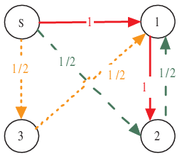
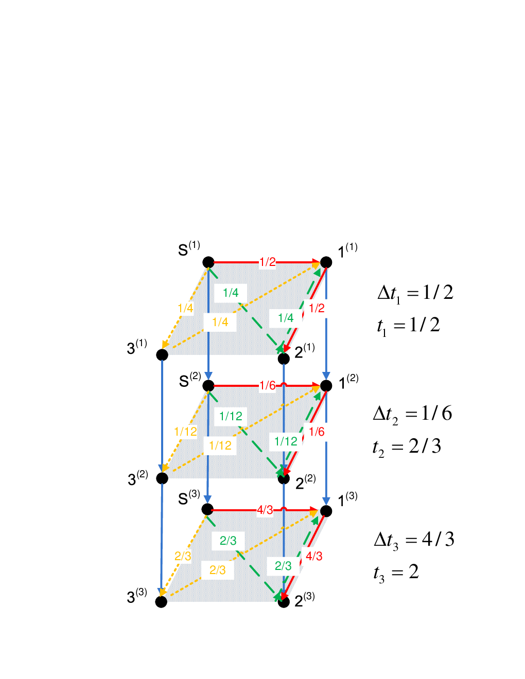
Fig. 2 gives one possible static rate allocation, showing the allocated rate for each edge of the original P2P graph . (Edges with zero allocated rate are not shown.) The source node transmits with a rate of 1 to peer 1 and with rate 1/2 to peers 3 and 4. Peer 1 transmits with rate 1 to peer 2 but does not transmit to any other peers. Peers 2 and 3 transmit with rate 1/2 to Peer 1, but do not transmit to any other peers.
Fig. 3 shows the time-expanded graph induced by the static rate allocation shown in Fig. 2. Because there are three peers, this time-expanded graph has 3 epochs. The peers are numbered in the order they finish downloading; peer 1 finishes first followed by peer 2 and then peer 3. The first epoch lasts time units, the second epoch lasts time units, and the third epoch lasts = 4/3 time units.
Peer 1 finishes first because it sees the full upload capacity of the source. As shown in Fig. 2 it sees rate 1 directly from the source. The other half of the source upload capacity is relayed to peer 1 by peers 2 and 3 immediately after they receive it. Hence peer 1 receives information with an overall rate of and finishes downloading the entire file, which has size at time . As a result, the duration of the first epoch is .
Peer 2 sees rate 1/2 directly from the source and rate 1 relayed to peer 2 by peer 1. Hence it sees an overall upload capacity of and finishes downloading the entire file at time . The duration of the second epoch can be computed as .
Because it receives no help from the other two peers, peer 3 sees an overall upload rate of only , which it receives directly from the source. It finishes downloading the entire file at time . The duration of the third epoch can be computed as .
The sum of the download times for the example of Figs. 2 and 3 is . Now let’s consider an example that minimizes the sum of the download times and in which peers finish at the same time.
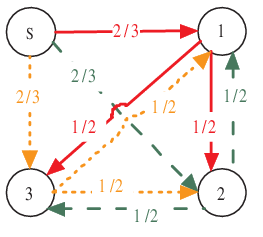
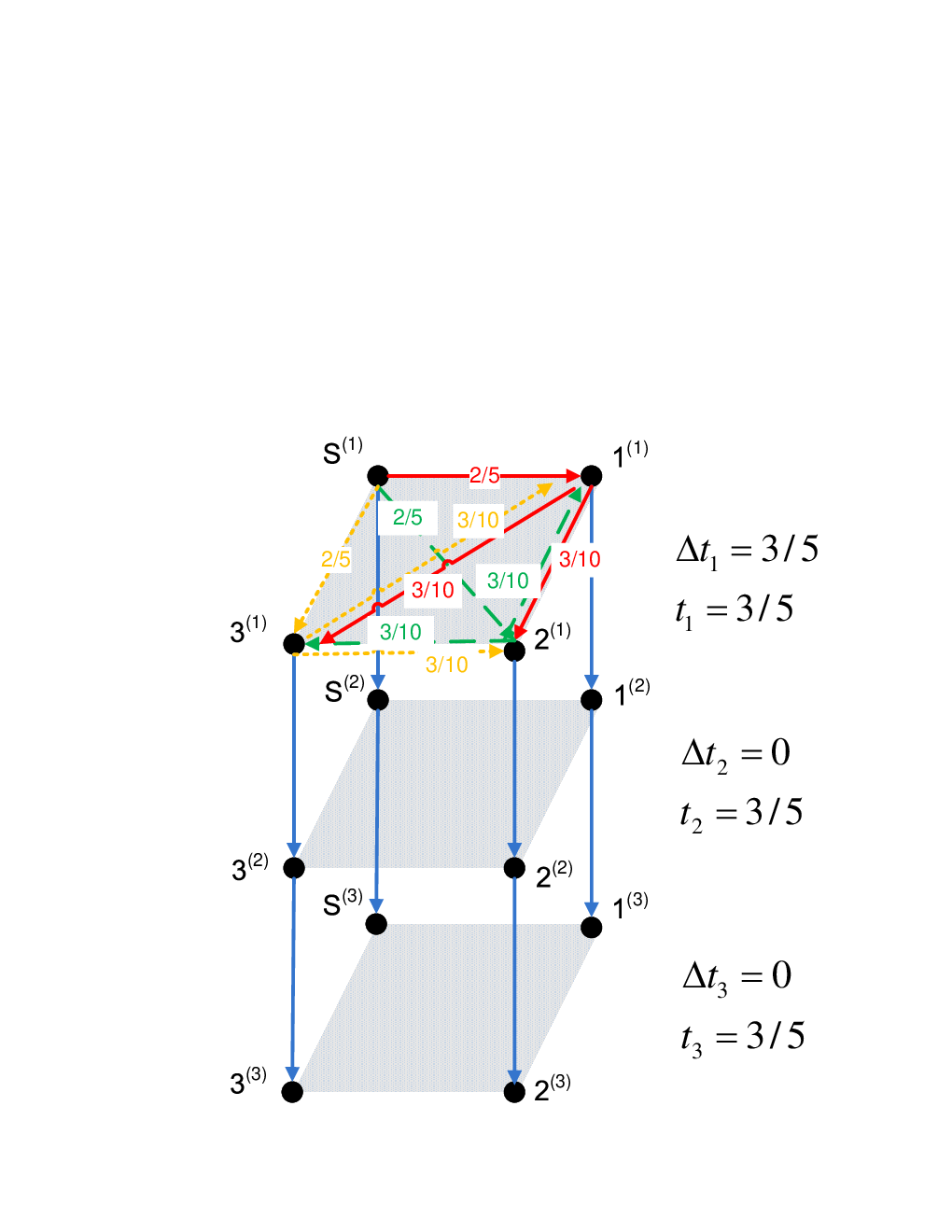
Fig. 4 shows the rate allocation that achieves the minimum possible sum of download times for a static allocation in this scenario, which turns out to be 1 4/5. The allocation shown in Fig. 4 is perfectly symmetric. Each peer receives rate 2/3 directly from the source and rate 1/2 from each of the two other peers. Each peer receives an overall rate of 5/3. Hence all three peers finish downloading simultaneously at and the second and third epochs have zero duration.
3.2 Transmission Flow Vectors and a Basic Network Coding Result
In Section 3.1 there was a tacit assumption that all of the information received by a peer is useful. For example, we assumed that the information relayed from peer 2 to peer 1 did not repeat information sent from the source to peer 1. In the examples of Section 3.1, one can quickly construct simple protocols that ensure that no critical flows are redundant. In this subsection, we review a general result that uses network coding theory to show that there is always a way to ensure that no critical flows are redundant.
Consider a general graph , which could be either a rate-allocation graph such as Figs. 2 or 4 or a time-expanded graph such as described in Figs. 3 and 5. Denote as the capacity of the edge . A transmission flow from the source node to a destination node is a nonnegative vector f of length satisfying the flow conservation constraint: ,where
| (3) |
The total flow supported by f is . This “flow” could be a flow rate with units of bits per unit time if we are considering a rate allocation graph such as Fig. 2 or it could be a total flow with units of bits or packets or files if we are considering a time-expanded graph such as Fig. 3.
As an example, the flow vector f describing the flow in Fig. 3 from (the source in the first epoch) to destination node (peer 2 in the second epoch, when peer 2 finishes downloading) has the nonzero elements shown in Table 1. Examining Table 1 verifies that the flow conservation constraint (3) is satisfied and that the total flow supported is equal to 1 file.
The following lemma states that a given fixed flow (or flow rate) can be achieved from the source to all destinations as long as there is a feasible flow vector supporting the desired flow from the source to each destination. i.e. We can achieve this flow to all destinations with network coding without worrying about possible interactions of the various flows..
Lemma 1
(Network Coding for Multicasting [21] [22]) In a directed graph with edge capacity specified by a vector c , a multicast session from the source node to a set of receivers can achieve the same flow for each if and only if there exits a set of flows such that
| (4) |
where is a flow from to with flow . Furthermore, if (4) holds, there exists a linear network coding solution.
3.3 A Convex Optimization
Given an order in which the peers will finish downloading, say peer finishes at the end of the -th epoch, applying Lemma 1 to the time-expanded graph with the set of destination nodes gives a characterization of all feasible downloading times, as concluded in the following lemma.
Lemma 2
(Feasible Downloading Times with Given Order [27]) Consider a P2P network in which node . Given an order in which the nodes will finish downloading a file with size , say node finishes at epoch , a set of epoch durations is feasible if and only if the following system of linear inequalities has a feasible solution:
| (5) | ||||
| g | (6) | |||
| (7) |
where is the uplink capacity of peer , and is a flow from first-epoch source node to node ’s termination-epoch node with flow rate .
As an example, the epoch durations of Fig. 3 are feasible because each of the flow vectors (one example was given in Table 1) satisfy the feasibility constraints of Lemma 2.
Let denote the download time to peer for . Given a static network resource allocation , as shown for example in Fig. 2, the maximum flow to peer , denoted as , is equal to the minimum cut between source node and peer in the rate-allocation graph (i.e. a graph such as Fig. 2, not the time-expanded graph). This follows from the Max-Flow-Min-Cut Theorem. Hence, .
From applying network coding results such as Lemma 1 to the rate allocation graph alone, we cannot conclude much about feasible download times since Lemma 1 addresses only the feasibility of the same flow to all destinations. However, by applying Lemma 1 to the time-expanded graph we can show that can be achieved simultaneously for all . Lemma 3 below states this result.
Lemma 3
Given a static network resource allocation , , for a P2P network, the only Pareto optimal (smallest) download time vector is for , where is the minimum cut from the source node to peer .
Proof 3.1.
It has been shown that for .
Hence, it is sufficient to show that for
is achievable. Without loss of generality, assume
that . Construct a static
scheme (i.e. a time-expanded graph ) as
follows:
(1) , where ;
(2) Flow capacity of edge is for and
;
(3) Flow capacity of edge is for ;
(4) Flow capacity of edge is infinity for and ;
(5) The destination nodes in the time-expanded graph are node
for . In other words, peer finishes at
the end of -th epoch.
According to the constructions (1) and (5), the download time to
peer is .
According to the constructions (2) and (3), in the subgraph
, the maximum flow from to is equal to
for all . Therefore, in this
time-expanded graph , the maximum flow from source node
to node is greater than or equal to
Therefore, by Lemma 1 and Lemma 2, there exists a linear network coding solution to multicast a file with size from the source node to peer within download time for all .
The maximum flow can be found by solving a linear optimization. Specifically, a set of flow rates is feasible if and only if there exists a solution to the following system of linear inequalities:
| (8) | ||||
| (9) | ||||
| (10) | ||||
| (11) |
| (12) | ||||
| (13) | ||||
| (14) | ||||
| (15) |
where () represents the network resource allocation and () is a flow from the source node to peer .
By Lemma 3, the minimum WSDT is the solution to the convex optimization of minimizing subject to (8-15). Thus, we can conclude the following theorem:
Theorem 1.
Consider multicasting a file with size from a source node to peers in a P2P network with both uplink and downlink capacity limits. The minimum weighted sum downloading time for the static scenario and the corresponding optimal static allocation can be found in polynomial time by solving the convex optimization of minimizing subject to the constraints (8-15).
Theorem 1 gives a solution to the most general static case that we are considering in this paper. However, it can be extended further by adding other linear network constraints (e.g. edge capacity constraints), which are not a concern of this paper.
3.4 The Uplink-Bandwidth-Sum Bound
For a P2P network with a source node and N peers, the convex optimization in Theorem 1 has variables and linear constraints. The complexity for the interior point method to solve this convex optimization is [29].
Even though the convex optimization can be solved in polynomial time, its complexity is still too high for practical applications when is large. Hence, bounds on the minimum WSDT and static schemes having network resource allocations that may be computed with low complexity are desired. In this subsection, we provide an analytical lower bound to the minimum WSDT with complexity for computing both the bound itself and the associated rate allocations.
Consider the cut of for any static allocation , the maximum flow rate from the source node to peer , , is limited by
| (16) |
and
| (17) | ||||
| (18) | ||||
| (19) |
Consider the cut of , is also bounded by
| (20) |
Inequalities (16) and (20) indicate that the downloading flow rate for peer is limited by peer ’s downlink capacity and the source node’s uplink capacity respectively. These two constraints are not only valid for the static scenario but also for dynamic scenarios.
Inequality (19) shows that the sum of the downloading flow rates for all peers is bounded by the total amount of the network uplink resource. Again, this constraint holds in both the static and dynamic cases.
These three constraints characterize an outer bound to the region of all feasible sets of satisfying (8 - 15). Therefore, for any static scheme, every set of feasible flow rates must satisfy (16), (19) and (20). However, not all satisfying (16), (19) and (20) are feasible.
Consider the following example: Let , , and (with ), the downloading flow rates satisfies the constraints (16), (19) and (20), but are not feasible because there is no solution to (8 - 15) with , i.e., no static scenario to support simultaneously. Specifically, for , all upload capability must be deployed, including that of peer 3. However, since , any transmission by peer 3 would violate the conservation-of-flow constraint.
Because all feasible sets of satisfy (16) (19) and (20), the solution to the following minimization problem provides a lower bound to the minimum WSDT for the static scenario:
| (21) |
where only are the variables. Empirical experiments presented in Section 5.5 show that this lower bound is tight for most P2P networks.
The minimization problem (21) is a convex optimization. Its optimal solutions are also the solutions to the associated KarushKuhnTucker (KKT) conditions [29]. The KKT conditions for problem (21) are
| (22) | ||||
| (23) | ||||
| (24) | ||||
| (25) | ||||
| (26) |
Solving the KKT conditions yields the following optimal solution for :
where is chosen such that
| (30) |
The lower bound to the WSDT for the static scenario is then
| (31) |
with as specified in (3.4).
For the special case where and , the solution given in (3.4) becomes
| (32) |
and the lower bound to the minimum WSDT is
| (33) |
Mutualcast [9] was designed to minimize the maximum download time for the case where . However, since Mutualcast can achieve the download time of for all peers, it achieves the lower bound of (31) for the case. This fact shows both that the lower bound of (31) is tight when and and that Mutualcast minimizes sum download time as well as the maximum download time when .
4 Mutualcast and Extended Mutualcast for the Equal-Weight Static Case
The concluding paragraph of Section 3.4 stated that Mutualcast minimizes the sum download time for the case where . In this section we extend Mutualcast to provide an algorithm we call Extended Mutualcast that handles finite constraints on (possibly delivering different rates to different peers) while still minimizing the sum download time.
4.1 Mutualcast
Mutualcast delivers the same rate to every peer. Assuming , Mutualcast can support peers with any rate . The key aspect of Mutualcast is that the source first delivers bandwidth to each node according to how much that node can share with all other peers. After that, if the source has any upload bandwidth left over, it is divided evenly among all peers. This leftover rate goes serves only one peer; it is not relayed to any other peers. Thus Mutualcast first forms a series of depth-two trees from the source to all nodes. Then, if there is any source upload bandwidth left over, it is used to form a series of depth-one trees. Here is a specification of the Mutualcast algorithm (without considering helper nodes):
Mutualcast delivers information to all peers at the same rate. As described in Algorithm 1 the highest rate that Mutualcast can deliver is
| (34) |
Consider two examples with ten peers, one in which and one in which .
First is an example where . Note that in general it is not possible for any peer to receive information at a rate higher than . Let , for all ten peers, and for all ten peers. Mutualcast achieves by having nine peers receive rate 1/9 from the source and forward at that rate to the nine other peers. One peer receives no information directly from the source because by the time the Mutualcast algorithm gets to that peer, the source upload bandwith has been used up.
For an example where , a larger is necessary. Let , for all ten peers and for all ten peers. Mutualcast achieves . In the first part of the Mutualcast algorithm, all ten peers receive rate 1/9 from the source and relay at that rate to the nine other peers. At this point there remains 80/9 of source upload bandwidth, which is distributed evenly so that each peer receives a rate of 8/9 directly from the source that it does not relay. In total, each peer receives rate 2 which is comprised of rate 1 from other peers, rate 1/9 from the source that it relays to the other peers, and rate 8/9 from the source that it does not relay.
The basic Mutualcast algorithm does not consider download constraints. The slight modification of Mutualcast given below includes download bandwidth constraints in the simplest possible way. Note that if all peers are to receive at the same rate, that rate must be less than the smallest download constraint. This is reflected in line 1 of Algorithm 2.
As with the original Mutualcast, Algorithm 2 delivers the same rate to every peer. This alone is enough to prevent it from minimizes the sum download time in general when there are download constraints. However, it will turn out to be an important component of Extended Mutualcast, which is an algorithm that does minimize the sum download time under general download constraints.
4.2 Extended Mutualcast
Setting for all in (3.4) produces the following lower bound on the sum download time when both upload and download constraints are considered:
| (35) |
where
| (38) |
where is chosen such that
| (39) |
This lower bound can be achieved by a routing-based scheme that we call Extended Mutualcast.
Consider a P2P network with constraints on peer uplink bandwidth and peer downlink bandwidth. Without loss of generality, assume that . Hence, and . The network resource allocation and the routing for Extended Mutualcast are provided in Algorithms 3 and 4 respectively.
The network resource allocation for Extended Mutualcast (Algorithm 3) is obtained by successively applying Algorithm 2 to the P2P network or part of the P2P network. The network resource allocation by Algorithm 3 has for all . The flow rate to peer , , is then equal to its download rate . The routing scheme for Extended Mutualcast (Algorithm 4) guarantees that the entire flow rate is useful. For the Extended Mutualcast rate allocation, so that the lower bound (35-39) on sum download time is achieved. Theorem 2 formally states and proves this fact.
Theorem 2.
Proof 4.1.
(Converse) From
(35-39),
is a lower bound on the minimum sum
download time. Hence, any sum download time less than
is not achievable.
(Achievability) It is sufficient to show that (a) Extended
Mutualcast is applicable to any P2P network, and (b) Extended
Mutualcast provides a static scenario in which the flow rate from
the source node to peer is of
(35-39).
(To Show (a)) It is sufficient to show that in Algorithm
3, the rate for each applied Algorithms
2 is attainable. In other words, each
rate for the applied network is less than or equal to the minimum of
the source node’s uplink capacity
and the total uplink resource over all of the peers.
- •
- •
If , consider the worst case of for and . In this case, we have
(40) (41) (42) (43) Denote as the total amount of the peers’ uplink resource used after Step , and as the total amount of the source node’s uplink resource used after Step . For Step 1, and . Hence, Algorithm 2 in Step 1 is feasible. Suppose Algorithm 2 is feasible for Step 1 to Step (). Then and . Hence,
(44) which indicates that Algorithm 2 for Step 1 to Step fully deploys the uplink resources of peers .
Now consider Algorithm 2 for Step , the supporting rate is . The source node’s uplink is . The total uplink resource is
(45) (46) (47) (48) where (46) follows from (43), and (48) follows from (42). Hence, the rate is less than or equal to the total available uplink resource (45) divided by the number of peers, . We also can see that is less than or equal to the available source node’s uplink bandwidth, . Therefore, Algorithm 2 for Step is also feasible. By induction, Algorithm 2 is feasible for every step.
- •
If , then
(49) (50) (51) Consider the worst case of . For this worst case, Algorithm 2 in Line 14 is feasible following an argument similar to that for the case of .
Therefore, Extended Mutualcast in Algorithm
3 is applicable to any P2P network.
(To Show (b)) From Algorithms 2
and 3, Extended Mutualcast constructs a
static scenario with for , and
. Hence, the maximum flow from the source node to peer is
larger than or equal to
| (52) | ||||
| (53) | ||||
| (54) |
Therefore, Extended Mutualcast provides a static scenario in which the flow rate from the source node to peer is of (35-39).
Theorem 2 showed that Extended Mutualcast minimizes the sum download time for any static P2P network. When the total uplink bandwidth resource is sufficiently abundant, Extended Mutualcast also minimizes the weighted sum download time for any set of weights because all peers are downloading at their limit of . Corollary 1 formally states and proves this fact.
Corollary 1.
Consider multicasting a file with size from a source node to peers in a P2P network with constraints on peer uplink bandwidth and peer downlink bandwidth. If , the set of the flow rates () is attainable. Hence, the minimum weighted sum download time for the static scenario is for any given weights .
Proof 4.2.
5 A Depth-2 Approach for the Minimizing Weighted Sum Download Time
Section 4 provided a complete solution (Extended Mutualcast) for achieving the minimum sum download time with constraints on both peer uplink bandwidth and peer downlink bandwidth. That section concluded by showing that if the total uplink resource is sufficiently abundant, Extended Mutualcast minimizes WSDT for any set of weights. This section attacks the minimization of WSDT more broadly.
Mutualcast and Extended Mutualcast construct only two types of trees to distribute content. The first type is a depth-1 tree as shown in Fig. 6(a). The source node broadcasts content to all peers directly with rate , . The second type is a depth-2 tree as shown in Fig. 6(b). The source node distributes content to peer with rate , and then peer relays this content to all other peers.

In Mutualcast, the rates are constrained to be equal for all . Also, for a fixed , for all . These constraints on the network resource allocation simplify the mechanism design and allow a simple routing-based scheme. These two constraints together ensure that each peer downloads content at the same rate. However, to optimize WSDT peers surely need to download content and different rates.
In Section 4 we saw that peers needed to download content at different rates to minimize the sum download time with peer downlink bandwidth constraints. The Extended Mutualcast algorithm provided a way to serve the peers at different rates corresponding to their download bandwidth constraints so as to minimize the sum download time. However, Extended Mutualcast required successive applications of Mutualcast which led to a complicated routing protocol.
In order to serve peers at different rates to minimize WSDT and still maintain a simple mechanism design, we apply the technique of rateless coding at the source node. A rateless code is an erasure correcting code. It is rateless in the sense that the number of encoded packets that can be generated from the source message is potentially limitless [30]. Suppose the original file size is packets, once the receiver has received any packets, where is just slightly greater than , the whole file can be recovered.
Fountain codes [30], LT codes [31], and raptor codes [32] are rateless erasure codes. LT codes have linear encoding complexity and sub-linear decoding complexity. Raptor codes have linear encoding and decoding complexities. The percentage of the overhead packets goes to zero as goes to infinity. In practice, the overhead is about 5% for LT codes with file size [30]. This sub-section focuses on applying rateless erasure codes for P2P file transfer instead of designing rateless erasure codes. Hence, we assume the overhead of the applied rateless erasure code is zero for simplicity. We note that if redundancy does not need to be limitless, there are solutions that provide zero overhead [33].
5.1 The Rateless-Coding-Based Scheme
We propose a rateless-coding-based scheme that constructs the two types of trees in Fig. 6 to distribute the content as did Mutualcast and Extended Mutualcast. The source node first partitions the whole file into chunks and applies a rateless erasure code to these chunks producing a potentially limitless number of chunks.
For the depth-1 tree, the source node broadcasts different rateless-coded chunks directly to each peer. For the depth-2 trees, The source node sends different rateless-coded chunks to each peer, and then that peer relays some or all of those chunks to other some or all of the other peers. A key point is that every chunk transmitted by the source is different from every other chunk transmitted by the source. This condition guarantees that all chunks received by a peer are useful (because they are not a repetition of a previously received chunk). Hence, a peer can decode the whole file as long as it receives coded chunks.
The rateless-coding-based scheme allows peers to download content at different rates with a simpler mechanism than the routing-based approach of Extended Mutualcast. Peers don’t have to receive exactly the same chunks to decode the whole file. Hence, the two types of tree structures can be combined as one tree structure with depth 2, but without the constraint that the rate from the peer to its neighbors has to equal the rate from the source to the peer.
The source node sends coded chunks to peer with rate , and peer relays some of them to peer () with rate . Note that the values of do not even need to be the same for a fixed value of and different values of .
Another benefit of applying a rateless coding approach is that it is robust to packet loss in the Internet if we allow some extra rate for each user.
Assuming rateless coding at the source node and constraining the P2P network to include only depth-2 trees as discussed above, the network resource allocation that minimizes WSDT can be obtained by solving the following convex optimization problem.
| (55) |
where . The complexity for the interior point method to solve this convex optimization is [29].
For the case of , the optimal resource allocation is, of course, the same as that of Mutualcast.
For the case of and finite values of , Algorithm 3 provides an optimal network resource allocation that certainly also solves (55). A key point is that the routing of Algorithm 4 becomes unnecessary if the source employs rateless coding. Peers need only relay the appropriate number of chunks to the appropriate neighbors without worrying about which chunks are relayed.
5.2 Resource Allocation for Networks with
Consider a P2P network in which peer uplink bandwidth is constrained but for . If , then the resource allocation of achieves the minimum WSDT with flow rates for all . (This is the case discussed at the end of Section 4.) Otherwise, consider the following water-filling-type solution:
| (56) |
where is chosen such that
| (57) |
The potential suboptimality of this approach comes from the subtraction of on the right side of (57) which does not appear in (30). Note that when (this is true for large ), is close to corresponding to the lower bound (3.4).
We now show that the proposed suboptimal network resource allocation ensures that the flow rate to peer is larger than or equal to of (56). Hence, the WSDT for the proposed suboptimal resource allocation is very close to the lower bound to the minimum WSDT for large networks.
First assign the rates for the depth-2 trees with
| (58) |
and
| (59) |
where is chosen to be the largest possible value satisfying
| (60) | ||||
| (61) |
Plugging (58) (59) into (60) (61), and obtain
| (62) |
where .
If , then the depth-2 trees have already fully deployed the source node’s uplink. The rate assignment for depth-2 trees is the network resource allocation for the rateless-coding-based scheme.
If , then the depth-2 trees have fully deployed all peers’ uplinks, but not the source node’s uplink. Hence, we can further deploy the rest of the source node’s uplink to construct the depth-1 tree. After constructing the depth-2 trees, the flow rate to peer is
The rest of the source node’s uplink is
The optimal depth-1 tree can be obtained by the convex optimization
| (63) |
The optimal solution to the problem (63) is
| (64) |
and
| (65) |
where is chosen such that (also ).
The complexity of calculating this suboptimal network resource allocation is . Note that when for all , this suboptimal network resource allocation is the same as that of Mutualcast, and hence, this network resource allocation is optimal for this case. For general weight settings, this network resource allocation guarantees that the flow rate to peer is larger than or equal to , which is stated in the following theorem.
Theorem 3.
Proof 5.1.
If , the flow rate to peer is
| (66) | ||||
| (67) | ||||
| (68) | ||||
| (69) | ||||
| (70) |
where (70) follows from . If , a feasible solution to problem (63) is
For this feasible solution, the total flow rate to peer with the depth-1 tree and the depth-2 trees is
| (71) | ||||
| (72) |
Denote . We have
| (73) | ||||
| (74) | ||||
| (75) | ||||
| (76) | ||||
| (77) |
Some of these steps are justified as follows:
- •
(73) follows from the fact that all uplink resource is deployed;
- •
(75) follows from the inequality when ;
- •
(76) follows from .
Therefore, . Hence,
| (78) |
which indicates that this feasible solution to the problem (63) provides a WSDT less than or equal to . Hence, the network resource allocation determined by (58) (59) (62) (64) and (65) also provides a WSDT less than or equal to .
5.3 Resource Allocation with Peer Downlink Constraints
Now we consider P2P networks with both peer uplink bandwidth constraints and peer downlink bandwidth constraints. The idea of the resource allocation for these P2P networks is the same as that for P2P networks without downlink constraints. The details are provided as follows:
If , consider a water-filling-type solution
| (79) |
where is chosen such that .
First construct the depth-2 trees with rates in (58) and (59), where is still chosen to be the largest possible value. However, for general P2P networks, the constraints on are not only (60) (61), but also
| (80) |
After constructing the depth-2 trees, the flow rate to peer is . The used source node’s uplink is . If , we can further use the rest of the source node’s uplink to distribute content through the depth-1 tree. The optimal resource allocation for the depth-1 tree can be obtained by the convex optimization
| (81) |
The optimal solution to the problem (81) is
| (82) |
and
| (83) |
where is chosen such that
The complexity of calculating this resource allocation is .
5.4 Routing-Based Depth-2 Scheme
So far, this section has provided a family of rateless-coding-based schemes for P2P file-transfer applications. In this subsection, we introduce a routing-based scheme. This routing-based scheme is a further extension to Extended Mutualcast. This scheme also applies the tree structures in Fig. 6 to distribute content. The constraints on the network resource allocation for this scheme are
| (84) |
and
| (85) |
where is the order in which the peers finish downloading. In the rest of this subsection, we assume the order is for simplicity. These constraints are stricter than those of the rateless-coding-based scheme, and they are introduced to simplify the routing scheme. In particular, given the order of in which peers finish downloading, the proposed routing-based scheme ensures that at any time in the scheme, peer has all packets received by peers for all . This condition can be achievable if the network resource allocation satisfies (84) and (85). For the routing-based scheme, when peer finishes downloading, the scheme starts to only broadcast the chunks which peer hasn’t received, called interesting chunks. With this condition, the interesting chunks are also new to peers . The details of the routing-based scheme is given in Algorithm 5.
The optimal network resource allocation for this routing-based scheme can be obtained by the convex optimization of minimizing subject to the constraints (84) (85), nodes’ uplink and downlink constraints, and the flow rate expression
where . The complexity for the interior point method to solve the problem is . For the case of and , the optimal network resource allocation is the same as that of Mutualcast. For the case of or , by Theorem 2 and Corollary 1, Algorithm 3 provides the optimal network resource allocation.
For general cases with , we provide a suboptimal network resource allocation for this routing-based scheme. Consider the water-filling-type solution in (79). Without loss of generality, assume that , and give the ordering in which the peers finish downloading. First construct the depth-2 trees with rates in (58) and (59), where is still chosen to be the largest possible value satisfying (60) (61) and (80). After constructing the depth-2 trees, the effective flow rate to peer is
| (86) | ||||
| (87) |
where . The download rate (used downlink) for peer is . Note that the effective flow rate is smaller than the download rate for peer . This is because peer only keeps a subset of chunks received from the source node. For this reason, parts of peer ’s downlink and the source node’s uplink are wasted. The total amount of the wasted uplink is
| (88) |
The used source node’s uplink is . If , we can further use the rest of the source node’s uplink to distribute content through the depth-1 tree. The constraints on the resource allocation for the depth-1 tree are (84),
| (89) |
and
| (90) |
Let . Let . A sub-optimal network resource allocation for the depth-1 tree is
| (91) |
and , where is chosen such that
and also
The complexity of calculating the suboptimal resource allocation for the routing-based scheme is .
5.5 Simulations for the Static Scenario
This subsection provides the empirical WSDT performances of the rateless-coding-based scheme, the routing-based scheme, and compares them with the lower bound to the WSDT. In all simulations, the file size is normalized to be 1. This subsection shows simulations for 6 cases of network settings as follows:
- •
Case I: , for ;
- •
Case II: , for ;
- •
Case III: , for ;
- •
Case IV: , for ;
- •
Case V: , for ;
- •
Case VI: , , ;
where is the indicate function.
Consider small P2P networks with peers. The performances of sum download time versus for these 6 cases are shown in Fig. 7. The performances of WSDT versus with weight () are shown in Fig. 8. The performances of WSDT versus with weight () are shown in Fig. 9. In all these simulations, the weighted sum download times of the rateless-coding-based scheme and the routing-based scheme achieve or almost achieve the lower bound.


Consider large P2P networks with peers. The performances of sum download time versus for these 6 cases are shown in Fig. 10. The performances of WSDT versus with weight () are shown in Fig. 11. The performances of WSDT versus with weight () are shown in Fig. 12. In all these simulations, the weighted sum download times of the rateless-coding-based scheme and the routing-based scheme also achieve or almost achieve the lower bound.


We also simulated for many other network settings and weight settings. In all these simulations, the rateless-coding-based scheme achieves or almost achieves the lower bound to the WSDT. Hence, the lower bound to the WSDT is empirically tight, and the rateless-coding-based scheme has almost-optimal empirical performance. The routing-based scheme also has near-optimal empirical performance. However, for few cases there are clear differences between the performance of the routing-based scheme and the lower bound.
6 The Dynamic Scenario
The dynamic scenario is allowed to re-allocate the network resource during the file transfer, in particular, whenever a peer finishes downloading, joins into the network, or leaves from the network.
6.1 A Piece-wise Static Approach to the General Dynamic Case
Wu et al. [27] show that to optimize WSDT the network resource allocation should be dynamic, but may remain constant during any “epoch”, a period of time between when one receiver finishes downloading and another finishes downloading. Thus, one optimal solution for the dynamic scenario is “piecewise static”.
As an example of how a “piecewise static” dynamic allocation can reduce the WSDT, consider the example for which we studied static allocations in Section 3.1. Recall that the example was for a P2P network with , and three peers with and . Fig. 13 shows the time-expanded graph corresponding to the optimal dynamic rate allocation for this example. Because there are three peers, this time-expanded graph describes a file transfer scenario with 3 epochs. The first epoch lasts 0.5 unit time. In the first epoch, the source node sends half of the file to peer 1 and the other half to peer 2. Peer 1 and peer 2 exchange their received content, and hence, both peer 1 and peer 2 finish downloading at the same time. Hence, the second epoch lasts 0 time units (since ). The third epoch lasts 0.25 unit time, in which the source node, peer 1 and peer 2 transmits to peer 3 simultaneously. Peer 1 sends a quarter of the file. Peer 2 sends another quarter. The source node sends the other two quarters.
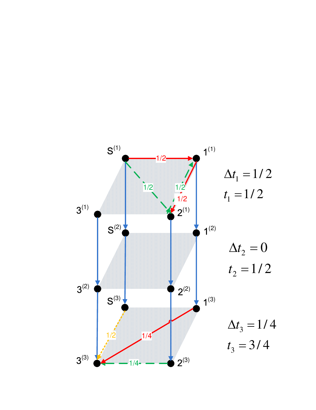
This dynamic solution turns out to achieve the minimum possible sum download time for this example which is 1.75. For comparison, the optimal static solution, which we saw in Section 3.1 had an only slightly larger sum download time of 1.8. This simple example shows that a dynamic rate allocation can reduce WSDT. In certain cases the benefit can be significant. Dynamic schemes can reduce the minimum sum download time to approximately half that of the static case, at least when downlink capacities are considered to be infinite [27].
6.2 A Rateless-coding Approach to Dynamic Allocation
Wu et al. [27] propose a dynamic routing-based scheme. This scheme first deploys all uplink resource to fully support the first peers until they finish downloading, where is appropriately chosen. After that, the scheme deploys all uplink resource to fully support the next peer until it finishes downloading, an so forth. Inspired by the work [27], we propose a dynamic rateless-coding-based scheme for P2P networks with both peer uplink bandwidth constraints and peer downlink bandwidth constraints. This scheme is applicable for dynamic P2P networks in which peers may even join or leave the network.
The key idea of this dynamic rateless-coding-based scheme is similar to that of the dynamic routing-based scheme in [27]. In particular, in each epoch, the scheme deploys all uplink resource to fully support several chosen peers. The details of the dynamic rateless-coding-based scheme are provided in Algorithm 6.
Algorithm 6 provides the structure of the dynamic rateless-coding-based scheme. Because the peers always receive independently generated rateless coded chunks in the static rateless-code scheme, the dynamic rateless-coding-based scheme is also applicable for dynamic P2P network. As long as a peer receives enough rateless coded chunks 11 1 The number of coded chunks needed to decode the whole file is only slightly larger than the total number of the original chunks., it can decode the whole file. The key issue is how to set the peers’ weights in each epoch. Since the weight setting and the static rateless-coding-based scheme in the current epoch will influence the dynamic scheme in the following epoches, the problem of setting weights is very complicated. We will address this problem in Section 6.3 and show that this problem is approximately equivalent to selecting a set of peers to fully support.
6.3 A Solution to the Ordering Problem
Wu et al. [27] demonstrate that given an order in which the receivers finish downloading, the dynamic allocation (neglecting downlink bandwidth constraints) that minimizes WSDT can be obtained in polynomial time by convex optimization and can be achieved through linear network coding. However, [27] leaves the proper selection of the ordering as an open problem and does not address the finite downlink capacities or the general case of weighted sum download time which allows any values of the weights .
The simulations for the static scenario in Section 5.5 show that the WSDT of static rateless-coding-based schemes are very close to that of the lower bound (3.4, 31). Hence, the flow rates in (3.4) are achievable or almost achievable by the static rateless-coding-based scheme. Recall that the constraints on the rate in (3.4) are
and
In the following discussion, we assume that any set of flow rates () satisfying the above constraints is achievable by the static rateless-coding-based scheme.
Consider one epoch of the dynamic rateless-coding-based scheme. Suppose there are peers in the network in the current epoch. Peer () has uplink capacity , downlink capacity and received rateless-coded chunks. Suppose the static rateless-coding-based scheme supports peer with flow rate () based on a weight setting. In order to find the optimal weight setting for the current epoch, we study the necessary conditions for the flow rates () to be optimal.
Let us first focus on two peers in the network, say peer 1 and peer 2. The total amount of the uplink resource supporting peer 1 and peer 2 is . If the flow rates for is optimal, then the flow rates and are also the optimal resource allocation for peers 1 and 2 given that the flow rates for are fixed. Now consider a suboptimal scenario in which the uplink resource with the amount of serves peers 1 and 2, and the rest of the uplink serves other peers in all of the following epoches. This suboptimal scenario provides a WSDT close to the minimum WSDT if (this is true for large ). Hence, we consider this suboptimal scenario and address the necessary conditions for and to be the optimal resource allocation for peers 1 and 2.
If , then peer 1 finishes downloading before peer 2 does. After peer 1 finishes downloading, peer 1 acts as a source node and hence the total amount of the source nodes’ uplink is , and peer 2 is supported by the uplink resource with the amount of . Hence, the WSDT for peers 1 and 2 is
| (92) |
and
| (93) |
Note that the sign of does not depend on . Hence, the optimal solution to is either (peer 1 and peer 2 finish at the same time) if , or (peer 1 is fully supported) if . Similarly, if , then peer 2 finishes downloading before peer 1 does. The WSDT for peers 1 and 2 is
| (94) |
and
| (95) |
Note that the sign of does not depend on eithter. Hence, the optimal solution to is either (peer 1 and peer 2 finish at the same time) if , or (peer 2 is fully supported) if . Therefore, the optimal resource allocation for peer 1 and peer 2 is achieved when one of the peers is fully supported, or they finish at the same time.
Lemma 4.
Given that the flow rates to peer for are fixed, and the amount of uplink resource supporting peer 1 and peer 2 is . If the optimal resource allocation for peer 1 and peer 2 is achieved when they finish at the same time, then both peer 1 and peer 2 are fully supported.
Proof 6.1.
Let and
. According to the above
discussion, the optimal resource allocation for peer 1 and peer 2 is
achieved when they finish at the same time if and only if ,
or and .
If , then ,
, and hence, peers 1 and 2 are
fully supported.
If and ,
then
and
. Hence, and . Multiply the above two inequalities and obtain
Therefor, peer 1 and peer 2 are also fully supported.
Corollary 2.
Given that the flow rates to peer for are fixed, and the amount of uplink resource supporting peer 1 and peer 2 is . The optimal resource allocation for peer 1 and peer 2 is achieved when one of them is fully supported or both of them are fully supported.
Corollary 3.
The optimal network resource allocation in each epoch of a dynamic scenario is only obtained when some peers are fully supported, at most one peer is partially supported, and the other peers are not supported.
Proof 6.2.
(proof by contradiction) If two peers are partially supported, say peer 1 and peer 2 are partially supported, then the resource allocation for peer 1 and peer 2 is not optimal by Corollary 2.
By Corollary 3, the optimal weight setting in each epoch is for the fully supported peers, for the partially supported peer, and for other peers. Hence, the problem of optimizing the weight setting is approximately equivalent to selecting a set of peers to fully support.
Now study the necessary conditions for a peer selection to be
optimal in a similar way. Suppose that the amount of uplink resource
supporting peer 1 and peer 2 is , and
the flow rates to peer for are fixed.
If and , then peer 1 finishes downloading if peer 1 is
fully supported, or peer 2 finishes downloading if peer 2 is fully
supported. When peer 1 is fully supported, the WSDT for peer 1 and
peer 2 is in (92) with .
When peer 2 is fully supported, the WSDT for these two peers is
in (94) with . Hence, we
have
| (96) | ||||
| (97) | ||||
| (98) |
Therefore, it is better to first fully support peer 1 if
when and
.
If and
, then peer 2 always finishes downloading
before peer 1 does. In this case, it is better to first fully
support peer 1 if , i.e.,
or approximately
If and , then peer 1 always finishes downloading before peer 2 does. In this case, it is better to first fully support peer 1 if , i.e.,
or approximately
These discussions are concluded in the following theorem.
Theorem 4.
Given that the amount of uplink resource supporting peer and peer is , and the flow rates to peer for are fixed. The optimal resource allocation for peer and peer is to fully support peer (i.e., ) if
| (99) |
Corollary 4.
Consider a peer selection for a dynamic scenario which selects peer to fully support and peer to not support. This peer selection is optimal only if
| (100) |
Proof 6.3.
Define the binary relation on as if (100) is satisfied. Denote a peer selection as where is the set of fully supported peers and is the set of unsupported peers. is optimal only if for any and . For general P2P networks, finding the optimal is computational impossible because the binary relation is not transitive, which means
Define the binary relation on as if . The binary relation is an approximation to the binary relation . is equivalent to when
| (101) |
It can be seen by plugging (101) into (100). The approximated binary relation has the transitive property, and hence, the peers can be ordered with respect to . Based on this ordering, a suboptimal peer selection algorithm and the corresponding weight setting is constructed as shown in Algorithm 7.
7 Simulations of the Dynamic Scenario
The dynamic rateless-coding-based scheme is feasible to both static P2P networks and dynamic P2P networks. Consider a type of dynamic P2P networks which any peer leaves from as it finishes downloading, and no peer joins into. This section provides the empirical WSDT performances of the dynamic rateless-coding-based scheme for static P2P networks and dynamic P2P networks with peer leaving, and compares them with those of the the static scenario for static P2P networks. In all simulations, the file size is normalized to be 1. This section shows simulations for Cases I,II,IV, and VI investigated in 5.5.


Consider median-size P2P networks with peers. The performances of sum download time versus for the 4 cases are shown in Fig. 14. Fig. 15 shows the relative value of the sum download time by normalizing the lower bound to be 1 in order to explicitly compare the performances of the dynamic rateless-coding-based scheme and the static scenario. For Case I where peers have infinite downlink capacities, the sum download time of the dynamic rateless-coding-based scheme is almost half of the minimum sum download time for the static scenario for a broad range of the source node uplink . This result matches the results in the previous work [27], which says that the minimum sum download time of dynamic scenarios is almost half of the minimum sum download time of static scenarios when node uplinks are the only bottleneck in the network. Our results also show that the sum download time of the dynamic rateless-coding-based scheme with peer leaving decreases to almost half of the minimum sum download time for the static scenario as increases. For Cases II, IV, and VI, the WSDs of the dynamic scheme and the dynamic scheme with peer leaving are also always smaller than the minimum WSDT for the static scenario. In particular, the WSDT of the dynamic scheme can be as small as 0.59, 0.70, and 0.73 of the minimum WSDT for the static scenario for Cases II, IV and VI, respectively. The WSDT of the dynamic scheme with peer leaving can be as small as 0.71, 0.82, and 0.86 of the minimum WSDT for static scenarios for Cases II, IV and VI, respectively. These largest improvements in percentage of deploying the dynamic scheme is obtained when the source node can directly support tens of the peers.
The performances of WSDT versus with weight () are shown in Fig. 16. Fig. 17 shows the relative value of the WSDT. For Case I, the sum download times of the dynamic rateless-coding-based scheme and the dynamic scheme with peer leaving can be even less than half of the minimum sum download time for the static scenario for a broad range of the source node uplink . This is because the peers with largest weight finish downloading first in the dynamic scheme. The WSDT of the dynamic scheme can be as small as 0.48, 0.49, and 0.58 of the minimum WSDT for the static scenario for Cases II, IV and VI, respectively. The WSDT of the dynamic scheme with peer leaving can be as small as 0.56, 0.62, and 0.77 of the minimum WSDT for the static scenario for Cases II, IV and VI, respectively. Note that for Case VI, the WSDT of the dynamic scheme with peer leaving is larger than that of the static scenario for small . This is because the peers with larger uplink resource also have larger weight, and they finish downloading and leave from the network first.


The performances of WSDT versus with weight () are shown in Fig. 18. Fig. 19 shows the relative value of the WSDT. For Case I, the sum download times of the dynamic rateless-coding-based scheme and the dynamic scheme with peer leaving is around half of the minimum sum download time for the static scenario for a broad range of the source node uplink . The WSDT of the dynamic scheme can be as small as 0.58, 0.55, and 0.52 of the minimum WSDT for static scenarios for Cases II, IV and VI, respectively. The WSDT of the dynamic scheme with peer leaving can be as small as 0.64, 0.64, and 0.63 of the minimum WSDT for the static scenario for Cases II, IV and VI, respectively. Note that for this weight setting, the WSDT of the dynamic scheme with peer leaving is always smaller than that of the static scenario for Case VI. This is because the gain by finishing peers with larger weight is more than than the loss by the peers with larger uplink resource leaving from the network.


Consider large P2P networks with peers. The performances of sum download time versus for the 4 cases are shown in Fig. 14. Fig. 15 shows the relative value of the sum download time. For Case I, the sum download time of the dynamic rateless-coding-based scheme is around 0.55 of the minimum sum download time for the static scenario for a broad range of the source node uplink . The sum download time of the dynamic rateless-coding-based scheme with peer leaving decreases to 0.70 of the minimum sum download time for the static scenario as increases to 1000. The WSDT of the dynamic scheme can be as small as 0.57, 0.70, and 0.70 of the minimum WSDT for the static scenario for Cases II, IV and VI, respectively.


8 Conclusion
This paper considers the problem of transferring a file from one source node to multiple receivers in a P2P network with both peer uplink bandwidth constraints and peer downlink bandwidth constraints. This paper shows that the static scenario can be optimized in polynomial time by convex optimization, and the associated optimal static WSDT can be achieved by linear network coding. Furthermore, this paper proposes static routing-based and rateless-coding-based schemes that closely approach a new lower bound on performance derived in this paper.
This paper also proposes a dynamic rateless-coding-based scheme, which provides significantly smaller WSDT than the optimal static scheme does. A key contribution for the dynamic scenario is a practical solution to the ordering problem left open by Wu. Our solution is to recast this problem as the problem of identifying the peer weights for each epoch of the “piecewise static” rate allocation.
The deployment of rateless codes simplifies the mechanism of the file-transfer scenario, enhances the robustness to packet loss in the network, and increases the performance (without considering packet overhead). However, there still exist several issues for rateless-coding-based scheme such as high source node encoding complexity, packet overhead, and fast peer selection algorithm for the dynamic scenario. The results of this paper open interesting problems in applying rateless codes for P2P applications.
The optimal download time region (set of optimal download times) for one-to-many file transfer in a P2P network can be characterized by a system of linear inequalities. Hence, minimizing the WSDT for all sets of peer weights leads to the download time region. The set of peer weights can also be assigned according to the applications. For instances, for a file transfer application with multiple classes of users, assign a weight to each class of users. For an application with both receivers and helpers, assign weight zero to helpers and positive weights to receivers. Hence, the results of this paper in fact apply directly to one-to-many file transfer applications both with and without helpers.
References
- [1] “BitTorrent.”. [Online]. Available: http://www.bittorrent.com.
- [2] “Napster.”. [Online]. Available: http://www.napster.com.
- [3] “Gnutella.”. [Online]. Available: http://www.gnutella.com.
- [4] “KaZaA.”. [Online]. Available: http://www.kazaa.com.
- [5] S. Androutsellis-Theotokis and D. Spinellis. “A survey of peer-to-peer content distribution technologies”. ACM Compl Surveys, 36(4):335–371, Dec. 2004.
- [6] J. Liu, S. G. Rao, B. Li, and H. Zhang. “Opportunities and challenges of peer-to-peer internet video broadcast”. Proceedings of the IEEE, Special Issue on Recent Advances in Distributed Multimedia Communications, 2007.
- [7] X. Zhang, J. Liu, B. Li, and T. S. P. Yum. “Coolstreaming/donet: A data-driven overlay network for efficient live media streaming”. in Proc. INFOCOM’05, 2005.
- [8] V. Pai, K. Kumar, K. Tamilmani, V. Sambamurthy, and A. E. Mohr. “Chainsaw: Eliminating trees from overlay multicast”. in Proc. 4th Int. Workshop on Peer-to-Peer Systems (IPTPS), Feb. 2005.
- [9] J. Li, P. A. Chou, and C. Zhang. “Mutualcast: An Efficient Mechanism for Content Distribution in a Peer-to-Peer (P2P) Network”. Microsoft Research, MSR-TR-2004-100, 2004.
- [10] J. Li. “PeerStreaming: A practical receiver-driven peer-to-peer media streaming system”. Microsoft, Tech. Rep. MSR-TR-2004-101, Sep. 2004.
- [11] Z. Xiang, Q. Zhang, W. Zhu, Z. Zhang, and Y.-Q. Zhang. “Peer-to-peer based multimedia distribution service”. IEEE Trans. Multimedia, 6(2):343–355, Apr. 2004.
- [12] J. Jannotti, D. K. Gifford, K. L. Johnson, M. F. Kaashoek, and J. W. O’Toole. “Overcast: Reliable multicasting with an overlay network”. in Proc. of the Fourth Symposium of Operating System Design and Implementation (OSDI), pages 197–212, Oct. 2000.
- [13] Y. Chu, A. Ganjam, T. S. E. Ng, S. G. Rao, K. Sripanidkulchai, J. Zhan, and H. Zhang. “Early experience with an internet broadcast system based on overlay multicast”. in Proc. of USENIX, 2004.
- [14] H. Deshpande, M. Bawa, and H. Garcia-Molina. “Streaming live media over a peer-to-peer network”. Stanford Univ. Comput. Sci. Dept., Tech. Rep., Jun. 2001.
- [15] X. Jiang, Y. Dong, D. Xu, and B. Bhargava. “GnuStream: A P2P media streaming system prototype”. in Proc. of 4th International Conference on Multimedia and Expo, Jul. 2003.
- [16] Y. Cui, B. Li, and K. Nahrstedt. “oStream: asynchronous streaming multicast in application-layer overlay networks”. IEEE J. Select. Areas Commun., 22(1):91–106, Jan. 2004.
- [17] V. N. Padmanabhan, H. J. Wang, and P. A. Chou. “Resilient peer-to-peer streaming”. Microsoft, Tech. Rep. MSR-TR-2003-11, Mar. 2003.
- [18] V. N. Padmanabhan, H. J. Wang, P. A. Chou, and K. Sripanidkulchai. “Distributing streaming media content using cooperative networking”. in Proc. NOSSDAV’02, May 2002.
- [19] K. Jain, L. Lovasz, and P. A. Chou. “Building scalable and robust peer-to-peer overlay networks for broadcasting using network coding”. Microsoft Research Technical Report MSR-TR-2004-135, Dec. 2004.
- [20] S. Accendanski, S. Deb, M. Medard, and R. Koetter. “How good is random linear coding based distributed networked storage?”. in Proc. 1st Workshop on Network Coding, WiOpt 2005, Riva del Garda, Italy, Apr. 2005.
- [21] R. Ahlswede, N. Cai, S.-Y. R. Li and R. W. Yeung. “Network information flow”. IEEE Trans. on Information Theory, 2000.
- [22] S.-Y. R. Li, R. W. Yeung, and N. Cai. “Linear network coding”. IEEE Trans. on Information Theory, 2003.
- [23] R. Koetter, M. Medard. “An Algebraic Approach to Network Coding”. IEEE Trans. on Networking, 2003.
- [24] D. Qiu and R. Srikant. “Modeling and Performance Analysis of BitTorrent-Like Peer-to-Peer Netowks”. In Proc. of SIGCOMM¡¯04, Portland, OR, Aug. 30 - Sep. 3 2004.
- [25] Z. Ge, D. R. Figueiredo, S. Jaiswal, J. Kurose, and D. Towsley. “Modeling peer-peer file sharing systems”. In Article of IEEE INFOCOM, 2003.
- [26] F. Clevenot and P. Nain. “A Simple Fluid Model for the Analysis of the Squirrel Peer-to-Peer Caching System”. In Article of IEEE INFOCOM, 2004.
- [27] Y. Wu, Y. C. Hu, J. Li, and P. A. Chou. “The Delay Region for P2P File Transfer”. in International Symposium of Information Theory 2009, Seoul Korea, July 2009.
- [28] J. Pouwelse, P. Garbacki, J. Wang, A. Bakker, J. Yang, A. Iosup, D. Epema, M. Reinders, M. van Steen, and H. Sips. “Tribler: A social-based Peer-to-Peer system”. The 5th International Workshop on Peer-to-Peer Systems, 2006.
- [29] S. Boyd and L. Vandenberghe. Convex Optimization. Cambridge Univ. Press, 2004.
- [30] D.J.C. MacKay. “Fountain codes”. in IEEE Proc.-Commun., (6), 2005.
- [31] M. Luby. “LT codes”. in 43rd Annual IEEE Symposium on Foundations of Computer Science, pages 271–282, 2002.
- [32] A. Shokrollahi. “Raptor codes”. “Technical report, Laboratoire d¡¯algorithmique, École Polytechnique Fédérale de Lausanne, Lausanne, Switzerland”, 2003, Available from algo.epfl.ch/.
- [33] T. Courtade and R. D. Wesel. “A deterministic approach to rate-compatible fountain communication”. IEEE Information Theory and Applications, 2010.